Seq2seq Translation Model for Sequential Recommendation

Abstract.

The context information such as product category plays a critical role in sequential recommendation. Recent years have witnessed a growing interest in context-aware sequential recommender systems. Existing studies often treat the contexts as auxiliary feature vectors without considering the sequential dependency in contexts. However, such a dependency provides valuable clues to predict the user’s future behavior. For example, a user might buy electronic accessories after he/she buy an electronic product.

In this paper, we propose a novel seq2seq translation architecture to highlight the importance of sequential dependency in contexts for sequential recommendation. Specifically, we first construct a collateral context sequence in addition to the main interaction sequence. We then generalize recent advancements in translation model from sequences of words in two languages to sequences of items and contexts in recommender systems. Taking the category information as an item’s context, we develop a basic coupled and an extended tripled seq2seq translation models to encode the category-item and item-category-item relations between the item and context sequences. We conduct extensive experiments on two real world datasets. The results demonstrate the superior performance of the proposed model compared with the state-of-the-art baselines.

1. Introduction

Recommendation system has become an inseparable part of our daily lives in the era of information explosion. A good recommendation system works like an information filter which can learn users’ interests based on their profile or preferences and then make proper predictions on their future behaviors. There are two main types of conventional recommendation systems, i.e., general recommenders and sequential recommenders. Researches on general recommendation mainly focus on modeling users’ general static preferences. Methods like matrix factorization (Koren et al., 2009) and BPR (Rendle et al., 2009) have shown impressive success towards this direction. However, in real-world scenarios, users’ future behavior can be greatly influenced by their current actions. Hence more recent studies have paid considerable interests on modeling such sequential behaviors.

The core of sequential recommendation lies in capturing the latent transition dependencies in users’ historical records. Many approaches (Tang and Wang, 2018; Yu et al., 2016; Wang et al., 2015; Kang and McAuley, 2018) try to model not only the interactions between users and items but also the evolution of users’ dynamic interests, and can get more accurate predictions compared with traditional methods. Markov Chains (MCs) are initially employed by building a transition matrix for sequential recommendation (Rendle et al., 2010). Afterwards, with the prevalence of deep learning techniques, many deep neural networks such as recurrent neural networks (RNN), convolutional neural network (CNN), and attention mechanism have also been incorporated into sequential recommender systems (Yu et al., 2016; Tang and Wang, 2018; Kang and McAuley, 2018). However, all these methods only concentrate on the item sequence itself without considering the rich context information.

The context information can provide new perspectives to understand users’ intrinsic intentions, and it has been proved helpful in improving the performance of sequential recommendation. Contexts can be viewed from both users’ and items’ perspective. The user’s contexts mainly consist of user’s profile information like age or profession and user’s actions like clicks  (Yao et al., 2017; Zhou et al., 2018; LE et al., 2018). It is usually hard to access users’ contexts due to the privacy protection issues, thus researchers pay more attention to items’ contexts  (He et al., 2017a; Bai et al., 2018; Huang et al., 2018a, b; Chang et al., 2018) such as category, brand, image, descriptions, or the location of a venue.

Existing studies have made considerable progress in modeling context information in sequential recommendation. However, most of these studies aim at learning fine-grained user or item representations with the help of contexts. For example, a number of approaches extract contextual features before sending them to the sequential recommendation module  (Yao et al., 2017; Bai et al., 2018; Zhou et al., 2018; Chen et al., 2019), and some approaches employ context-specific matrices to capture the temporal and spatial contexts in location prediction  (Liu et al., 2016b, a). The aforementioned methods are all built upon the single item sequence without considering the latent transition patterns in contexts. In other words, they concentrate on the sequential modeling of the items and ignore the dynamics of additional contexts. It is worth mentioning that though STAR  (Rakkappan and Rajan, 2019) apples two RNN sequences or two matrices to model the sequences of item and context respectively, the transition patterns in contexts are not explicitly exploited. Moreover, the context and item sequence are treated separately without considering their relations in these two sequences.

In this paper, we argue that the sequential dependency in contexts provide valuable clues to predict the user’s future intentions. We first present an example of category level and item level transition pattern in Figure  1. We choose the category as an items’ context since the category information is easily accessible in most of real world e-commerce web sites or online social networks. Also, the category-level transition can be indicative in determining the user’s decision process. For example, when a visitor arrives at a new city, he/she is more likely to go to a hotel for a rest than to shop in a mall. Hence a clever system should learn to recommend a hotel list rather than a mall list based on the current context.

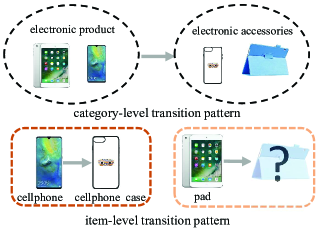
Figure 1. The category- and item- level transition patterns.

Fig.  1 shows that a specific user once purchased a $phone\ case$ after he/she bought a $cellphone$ and there is an item-level transition from cellphone to cellphone case. Such an item dependency might be not very informative for future prediction when the user buys a pad. However, the category level transition from electronic product to electronic accessories will help the system to recommend pad case to the user. While being aware of the importance of category-level transition, the main challenge is how to capture the transition patterns in item sequence and those in category sequence independently, and to maintain the relationship between two sequences at the same time.

To tackle these problems, we propose a novel seq2seq translation modeling for context-aware sequential recommendation in this work. Our idea is inspired by the recent advancement in NMT (neural machine translation). The target of NMT is to translate a source sentence from one language to the target one in another language. NMT not only models the sequential patterns but also captures the semantic relations between two corpora.

Intuitively, we can treat the item and category sequences as two sentences in different languages and model their relations in a translation way. However, there are still two big gaps between the scenarios in language and recommendation translation. On one hand, a NMT model usually reads the source sentence as a whole then outputs the target. In recommendation, we cannot foresee the future information which means an information leakage and may lead to overfitting. On the other hand, each word from the source corpus is in parallel with one corresponding word in the target corpus. While in our case, a category may contain a number of items which indicates a subsidiary relationship. Hence we further present a one-by-one strategy to match the source and target sequences one by one and design a variational auto-encoder as an information filter to model the subsidiary relationship between the item and category.

To summarize, the major contributions of this work are as follows.

• We highlight the importance of exploring the category-level transition patterns in sequential recommendation. To the best of our knowledge, this has been not exploited in the previous literature.

• We develop a basic coupled and an extended tripled seq2seq translation models to capture item-level and category-level transition patterns independently and maintain the relations between item and category sequences in a translation way.

• Extensive experiments over two different public datasets show that the proposed model significantly outperforms the state-of-the-art methods for the sequential recommendation task.

2. Related Work

This section reviews the literature in sequential recommendation and the related neural translation models.

2.1. Deep Learning based Sequential Recommendation

The powerful modeling capacity of deep learning techniques has opened up new opportunities for sequential recommendation whose core task is to predict users’ future actions based on previous interactions.

There are a number of pioneer significant works using various deep neural networks and they have shown the improvements over the traditional methods. Recurrent neural network which is originally designed for sequential data, has been widely applied in the sequential recommendation problem. For instance, RNN is employed in DREAM (Yu et al., 2016) to capture the global transition features from users’ transaction baskets. Hidasi et al. (Hidasi et al., 2015) propose to apply Gated Recurrent Unit, a variety of RNN, to the session-based recommendation. Despite RNN, convolutional neural network is also adopted in CASER (Tang and Wang, 2018) to deal with union-level skip patterns. Recently, self-attention technique (Vaswani et al., 2017) is shown to exhibit promising performance in many fields such as computer vision and natural language processing. As a result, several sequential recommendation approaches such as SASRec (Kang and McAuley, 2018) and ATTRec (Zhang et al., 2019) leverage self-attention mechanism to identify relevant items from history. Other kinds of DNNs like memory network (Chen et al., 2018) and gating mechanism (Chen Ma and Liu, 2019) are also widely employed in the literature. Generally, these deep learning based methods mainly concentrate on item sequence modeling without considering any context information.

2.2. Context-aware Sequential Recommendation

In addition to mining the interaction sequences, researchers are paying more attentions to additional context information to improve the performance. Specifically, CA-RNN (Liu et al., 2016b) builds two adaptive context matrices to capture the input (weather, category) and transition (distance, time intervals) contexts respectively. Bai et al. (Bai et al., 2018) employ an attention mechanism to exploit users’ evolving appetite for items’ attributes. Zhou et al. (Zhou et al., 2018) propose an attention-based framework ATRank which models the users’ heterogeneous behaviors. CSAN (Huang et al., 2018a) is proposed based on ATRank to discriminate the significance of individual user behaviors. AIR  (Chen et al., 2019) collectively exploits the rich heterogeneous user interaction actions through the category information. The above methods are all in the E-commerce scenario. In POI recommendation, LBPR (He et al., 2017a), SREM (Yao et al., 2017), and CAPE (Chang et al., 2018) take either the category or textual information into consideration.

The aforementioned approaches are all based on the single interaction sequence. Recently, a few multi-sequence based context-aware methods have been proposed. Le et al. (LE et al., 2018) develop three twin network structures to capture the synergies between support (e.g., clicks) and target (e.g., purchases) sequences through fully or partial sharing parameters. STAR (Rakkappan and Rajan, 2019) makes use of stacked RNNs to model item and context sequences, respectively. Overall, capturing transition patterns in context is attracting more attention. However, none of existing methods models them in an explicit way. Meanwhile, the relation between the interaction sequence and the context sequence has been not exploited in these approaches. In contrast, we propose to model context sequential patterns and maintain relations between category and item at the same time.

2.3. Neural Machine Translation Methods

Our method is mainly inspired by the machine translation problem whose target is to translate large amounts of texts from the source languages into ones in the target languages. Benefited from deep neural networks, neural machine translation has achieved great success based on seq2seq architecture  (Sutskever et al., 2014) compared with traditional statistical approaches. Self-attention mechanism is also fully utilized to boost the performance (Luong et al., 2015; Bahdanau et al., 2014).

There are mainly three components in a NMT model: an encoder for source sentence reading, a decoder for target sentence generating, and a middle-ware for relation modeling. The encoder and decoder are usually modeled with recurrent neural networks and the middle-ware with an attention mechanism. It is clear that NMT method not only models relations between two corpora but also explores multi-sequential patterns independently which is inherently identical to our problem.

Variational Auto-Encoder

Variational auto-encoder is a widespread generative model proposed by Kingma et al. (2013). Many studies have applied VAE to other fields such as recommendation system (Liang et al., 2018; Sachdeva et al., 2019) and neural machine translation (Zhang et al., 2016). The powerful generative capacity of VAE enables a method to go beyond the limited modeling ability of linear factor models. Due to the sampling process, incorporating variational auto-encoder can improve the robustness of previous deep neural network based model and boost the performance. More recently, an extended version $\beta$-VAE (Higgins et al., 2017) is proposed by introducing a hyper-parameter $\beta$ to emphasize the regularization term. It is demonstrated that $\beta$-VAE can learn interpretable factorized latent representations and outperform basic VAE with $\beta\geq 1$. In our work, we also take advantage of variational auto-encoder’s generative capacity to better capture the relation between the item and category sequences.

3. Problem Formulation

In this section, we introduce the problem formulation and then present the preliminary neural machine translation (NMT) Model.

3.1. Problem Formulation

Assume that we have a set of users and items denoted by $U=\left\{u_{1},u_{2},...,u_{|U|}\right\}$ and $I=\left\{i_{1},i_{2},...,i_{|I|}\right\}$ where $|U|$ and $|I|$ are the numbers of users and items, respectively. For each user $u\in U$, we can obtain a sequence of his/her behaviors sorted by time $s_{ui}=\left\{i^{u}_{1},i^{u}_{2},...,i^{u}_{t}\right\}$, where $i^{u}_{t}$ denotes the item purchased or rated at time step t by the user $u$.

In this study, we focus on the problem of context-aware sequential recommendation, where each item $i$ that the user $u$ interacts with at time t may contain various types of additional context information. In our paper, we are mainly interested in the category information for the item and take it as the item’s context. Let $C=\left\{c_{1},c_{2},...,c_{|C|}\right\}$ as the category set, where $|C|$ is the number of categories and each item $i$ always belongs to a specific category $c$. Note that our architecture can be easily extended to model other additional context information.

Given the item sequence $s_{ui}=\left\{i^{u}_{1},i^{u}_{2},...,i^{u}_{t}\right\}$ that the user $u$ interacts in the history, and the corresponding category sequence $s_{uc}=\left\{c^{u}_{1},c^{u}_{2},...,c^{u}_{t}\right\}$, the goal of context-aware sequential recommendation is to predict the item $i^{u}_{t+1}$ that the user $u$ is most likely to interact with at the next $t+1$ time step. For ease of presentation, we list the notations in this paper in Table  1.

Table 1. List of notations.

Notation	Description
$U$	a set of all users
$I$	a set of all items
$C$	a set of all categories
$\bm{u}$	the embedding of a user $u$
$\bm{i}$	the embedding of an item $i$
$\bm{c}$	the embedding of a category $c$
$d$	the dimension of embeddings and the hidden states
$\bm{h}$	the hidden state vector
$\bm{W}$	the weight matrix learned during training

3.2. Preliminary: Neural Machine Translation (NMT) Model

The main target of machine translation is to read a sentence like $``I\ like\ watching\ war\ movies"$ and produce $``Ich\ schaue\ gerne\ Filme"$ as the output sentence using the English to Czech task as an example which can also be considered as a seq2seq task. The overview of a classic neural machine translation model is shown in Figure 2.

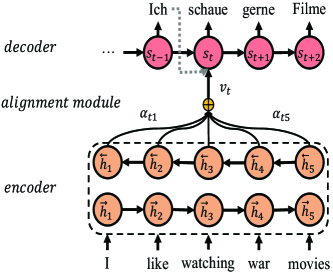
Figure 2. Neural Machine Translation (NMT) Model

As shown in Fig. 2, the NMT framework can be briefly described as an encoder-decoder architecture where the encoder reads the whole source sentence and the decoder translates the outputs of encoder to the target sentence. For encoder, previous works usually employ a bidirectional recurrent neural network that reads the whole source sentence $(\bm{x_{1}},\bm{x_{2}},...,\bm{x_{T_{x}}})$ in a context-aware way, where $\bm{x_{n}}$ is the embedding of word $x_{n}$. It will output a sequence of hidden states $(\bm{h_{1}},\bm{h_{2}},...,\bm{h_{T_{x}}})$ where $\bm{h_{t}}$ contains context information around word $x_{t}$ and can be calculated as:

(1) $$\overrightarrow{\bm{h_{t}}}=\overrightarrow{{\rm RNN}}(\bm{h_{t-1}},\bm{x_{t}}),$$

(2) $$\overleftarrow{\bm{h_{t}}}=\overleftarrow{{\rm RNN}}(\bm{h_{t+1}},\bm{x_{t}}),$$

(3) $$\bm{h_{t}}=\overrightarrow{\bm{h_{t}}}\oplus\overleftarrow{\bm{h_{t}}},$$

where $\oplus$ denotes vector concatenation.

There is an alignment module or so called attention module deciding which part of the source sentence should be focused on. The alignment module is based on the current decoding stage and will derive a context vector $\bm{v}$:

(4) $$\bm{v_{(t-1)j}}=\sum_{j=1}^{T_{x}}\alpha_{(t-1)j}\bm{h_{j}},$$

(5) $$\alpha_{(t-1)j}=\frac{{\rm exp}(e_{(t-1)j})}{\sum_{k=1}^{T_{x}}{\rm exp}(e_{(t-1)k})},$$

where $\alpha$ is the weight parameter, and $e_{(t-1)j}$ measures how well the decoding stage at position t-1 and the input hidden state at position j match, and it can be formulated as:

(6) $$e_{(t-1)j}=p(\bm{s_{t-1}},\bm{h_{j}}),$$

where $\bm{s_{t-1}}$ is the hidden state in the decoder which will be defined later, and $p$ is the function that can be defined in many ways such as a multi-layer perceptron.

After the alignment procedure, the decoder starts to generate the target word given the previous predicted words $(y_{1},y_{2},...,y_{t-1})$ and the current context vector $\bm{v_{t}}$ commonly through a directional recurrent neural network. It will first calculate the hidden state $\bm{s_{t}}$ of the decoding stage at the time t:

(7) $$\bm{s_{t}}={\rm RNN}(\bm{s_{t-1}},\bm{v_{t}},\bm{y_{t-1}}),$$

where $\bm{y_{t-1}}$ is the vector for the (t-1)-th word $y_{t-1}$.

Then the probability of choosing the next word $y_{t}$ is generally defined as:

(8) $$\small p(y_{t}|y_{<t};(x_{1},x_{2},...,x_{T_{x}}))=f(\bm{s_{t}},\bm{v_{t}},\bm{y_{t-1}}),$$

where the function $f$ aims to fuse information from three sources including the current hidden state $\bm{s_{t}}$, the current context vector $\bm{v_{t}}$, and the previous word vector $\bm{y_{t-1}}$, and gives the final probability score.

Overall, the basic NMT method can model two sequences independently and builds a bridge between them, showing that it can capture the sequential patterns in the source and target sentences as well as reflect the relation between two sentences. Based on this observation, we introduce the seq2seq language model to the sequential recommendation field.

4. The Proposed Model

In this section, We elaborate the proposed architecture in detail. We first present a basic coupled seq2seq translation model (CSTM), and then extend it to a tripled seq2seq translation model (TSTM).

4.1. Coupled Seq2seq Translation Model

The key idea of our modeling is to treat the category and item sequences as two sentences to be translated. Different from previous approaches, we aim to extract two types of transition patterns from item and category sequences independently while keeping relations between these two sequences. Taking the example in Fig. 1 for illustration, the item-level transition $cellphone$ $\rightarrow$ $cellphonecase$ and the category-level transition $electronic$ $product$ $\rightarrow$ $electronic$ $accessories$ are two different but inherently associated patterns. When the user later buys a pad in $electronic$ $product$, it would be indicative to first choose the correct category $electronic$ $accessories$ and then recommend the right item $pad$ $case$.

Inspired by the NMT mechanism, we propose to model the items and categories as two sentences in two corpus, where the item-level and category-level transition patterns are encoded in two word sequences, and the relation between item and category sequence is captured by the translation process.

In this section, we first present a basic coupled seq2seq translation model (CSTM) which directly translates category sequence into item sequence. CSTM aims to reflect the scenario where the users first decide the item category and then choose the item. For example, when a user wants to buy some fruits, he/she will browse the webpages containing various fruits like oranges and apples and then make the selection. The architecture of CSTM is shown in Figure 3.

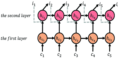
Figure 3. Coupled Seq2seq Translation Model (CSTM)

Similar to the NMT method, there are two main components in CSTM: the first layer and the second layer. Please note that we use the $first$, $second$, and $third$ layer instead of encoder and decoder to refer to different parts in our model because we will introduce multi-layers in the following section.

Different from the bidirectional RNN in NMT, we propose a one-by-one strategy to translate each category into an item instead of operating on whole sentence. The details are as follows. In the first layer (encoder) in CSTM in Fig.  3, we apply a single forward RNN, rather than the bi-directional RNN in NMT, to the input category sequence. In the language translation scenario, the bi-directional RNN are beneficial to the target sentence generation. By reading the whole source sentence in a back and forward way, it increases the awareness of the main intention. However, the nature of sequential recommendation task is quite different. When we are going to predict which item the user will interact at the next step, we cannot be informed of the next category in advance. Hence we should not model the category sequence with bi-directional RNN which encodes the information of the whole source sentence.

In the second layer (decoder) in CSTM in Fig.  3, given the fact that we know the first category $c_{1}$ and its corresponding item $i_{1}$, our goal is to predict the next item $i_{2}$. This is also different from that in NMT which tries to find a word in the target corpus with the same meaning, e.g., $I$ to $Ich$, and $movie$ to $Filme$, showing a mapping from $(s_{1},s_{2},s_{3},s_{4},s_{5})$ to $(t_{1},t_{2},t_{3},t_{4},t_{5})$. In contrast, in our case, we are going to translate the sequence $(c_{1},c_{2},c_{3},c_{4},c_{5})$ into $(i_{2},i_{3},i_{4},i_{5},i_{6})$.

We now present the detail in adapting NMT to our next item prediction problem. Specifically, in Fig.  3, the first layer takes a sequence of category $(\bm{c_{1}},\bm{c_{2}}$,…,$\bm{c_{t}})$ as the input, where $\bm{c_{i}}\in\mathbb{R}^{d\times 1}$ is the embedding of the i-th category $c_{i}$ and $d$ is the dimension size of embedding. The output is a hidden category state sequence $(\bm{h_{c1}},\bm{h_{c2}}$,…,$\bm{h_{ct}})$ where each $\bm{h_{c_{t}}}\in\mathbb{R}^{d\times 1}$ is calculated as:

(9) $$\bm{h_{c_{t}}}={\rm RNN}(\bm{h_{c_{t-1}}},\bm{c_{t}})$$

We then input the hidden category states into the second layer directly, without going through the commonly used alignment module in NMT. As we have analyzed before, we should not get any explicit clues from future, whereas the output of the alignment module will contain information about the whole input sentence, and this may lead to information leakage and overfitting.

Another issue in the second layer is that we would like to take the category information into account due to the correlation between the category and the item. From the category perspective, $\bm{h_{c_{t}}}$ is the category state mostly relevant to the next item $i_{t+1}$. Thus we define the hidden item state $\bm{h_{i_{t}}}\in\mathbb{R}^{d\times 1}$ in the second layer in CSTM as follows:

(10) $$\bm{h_{i_{t}}}={\rm RNN}(\bm{h_{i_{t-1}}},\bm{i_{t}},\bm{h_{c_{t}}}),$$

where $\bm{h_{i_{t-1}}}\in\mathbb{R}^{d\times 1}$ is the (t-1)-th hidden item state, $\bm{i_{t}}\in\mathbb{R}^{d\times 1}$ is the embedding for the t-th item, $\bm{h_{c_{t}}}\in\mathbb{R}^{d\times 1}$ is the t-th hidden category state.

To train the model, we maximize the point-wise ranking loss function at the step t which can be formulated as the log likelihood:

(11) $$\mathcal{L}=\mathcal{L}_{1}+\mathcal{L}_{2}$$

(12) $$\mathcal{L}_{1}={\rm log}(p(\bm{i_{t+1}}|\bm{h_{i_{t}}})),$$

(13) $$\mathcal{L}_{2}={\rm log}(p(\bm{c_{t+1}}|\bm{h_{c_{t}}})),$$

The loss $\mathcal{L}$ at step t consists of two terms: $\mathcal{L}_{1}$ for the next item prediction and $\mathcal{L}_{2}$ for the next category prediction. The probability $p(\bm{i_{t+1}}|\bm{h_{i_{t}}})$ and $p(\bm{c_{t+1}}|\bm{h_{c_{t}}})$ in Eq.  12 and Eq.  13 can be calculated by adding softmax layers over the hidden category and item state $\bm{h_{i_{t}}}$ and $\bm{h_{c_{t}}}$, respectively:

(14) $$p(\bm{i_{t+1}}|\bm{h_{i_{t}}})={\rm softmax}(\bm{W_{1}}\bm{h_{i_{t}}})$$

(15) $$p(\bm{c_{t+1}}|\bm{h_{c_{t}}})={\rm softmax}(\bm{W_{2}}\bm{h_{c_{t}}})$$

where $\bm{W_{1}}\in\mathbb{R}^{|I|\times d}$, $\bm{W_{2}}\in\mathbb{R}^{|C|\times d}$ are trainable parameters. It is worth noting that there is only one loss function for target sentence prediction in original NMT model. Our recommendation problem is much more difficult since the future information is unknown. We add the category loss $\mathcal{L}_{2}$ in our case so as to make the proposed method to have the ability to predict the category, which in turn help predict the item.

4.2. Tripled Seq2seq Translation Model

In the previous section, we design a basic CSTM to directly utilize the category-level transition pattern for the prediction of the next item. However, the relation between the item-level and category-level transition patterns is not fully explored due to the one-way information passing from category to item. While treating category as auxiliary information helps item prediction, the item can also assist the category prediction in a reverse way. Inspired by the concept of back-translation (Sennrich et al., 2015), we further propose an extended tripled seq2seq translation model (TSTM).

The key idea of TSTM is to translate item sequence into category sequence at the first stage and then translate it back to item sequence at the second stage. We believe that item and category sequences can unite tightly and benefit from each other during the generating process. In other words, item sequence can help predict category more precisely and the generated high-quality category sequence can improve the item prediction.

Intuitively, it would be easy to translate the item sequence into the category sequence. However, due to the subsidiary relationship between category and item, i.e., category is an abstract and high-level description about the specific item, it is hard to translate item sequence $(i_{1},i_{2},i_{3},i_{4},i_{5})$ into category sequence $(c_{2},c_{3},c_{4},c_{5},c_{6})$ by directly applying the NMT model, where the source and the target word are of the same semantic level. To address the problem, we introduce a generative variational auto-encoder (Kingma and Welling, 2013) (VAE) as an information filter to model such a subsidiary relationship.

VAEs have been widely used in language modeling and recommendation (Zhang et al., 2016; Liang et al., 2018; Sachdeva et al., 2019) owing to the power of learning a compressed representation $\bm{z}$ of the input picture or input sequence. The conventional loss function of the VAE  (Kingma and Welling, 2013) is formulated as:

(16) $$L=-D_{KL}(q(\bm{z}|\bm{x})||p(\bm{z}))+\mathbb{E}_{q(\bm{z}|\bm{x})}[{\rm log}(p(\bm{x}|\bm{z}))],$$

where $\bm{x}$ is the input observed data, $\bm{z}$ is the latent factor variable, $q(\bm{z}|\bm{x})$ and $p(\bm{x}|\bm{z})$ are inference and generative model, and $D_{KL}(q||p)$ is the Kullback-Leibler divergence between two distributions. In Eq. 16, the expectation part $\mathbb{E}$ can be viewed as reconstruction loss while the KL part as regularization. Furthermore, $\beta$-VAE introduces a hyper-parameter $\beta$ to push the model to learn a disentangled representation of the data:

(17) $$L=-D_{KL}(q(\bm{z}|\bm{x})||p(\bm{z}))+\beta\mathbb{E}_{q(\bm{z}|\bm{x})}[{\rm log}(p(\bm{x}|\bm{z}))]$$

In order to model the subsidiary relationship between the category and item, we employ a continuous latent variable $\bm{z}$ at each step in item sequence, which will decide what category the next item should be selected from. By introducing the variable $\bm{z}$, we can sample an item which belongs to the same category of the previous item at the next time step. This will help the category prediction more robust. Based on the above assumption, we design our VAE incorporated tripled seq2seq translation model. The architecture of TSTM is shown in Figure 4.

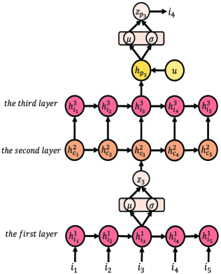
Figure 4. Tripled Seq2seq Translation Model (TSTM)

TSTM mainly consists of three layers in Figure 3. The first layer reads the item sequence, then the second layer translates the item into category, and finally the third layer back translates category into item. Before the second layer and the final prediction, there are two VAEs processing the output of the first layer and the third layer, respectively.

Specifically, we feed the item embedding sequence $(\bm{i_{1}},\bm{i_{2}},...,\bm{i_{t}})$ to the first layer and get the output of hidden item state $\bm{h^{1}_{i_{t}}}\in\mathbb{R}^{d\times 1}$ at step t:

(18) $$\bm{h^{1}_{i_{t}}}={\rm RNN}(\bm{h^{1}_{i_{t-1}}},\bm{i_{t}})$$

$\bm{h^{1}_{i_{t}}}$ is then used for next item prediction in the first layer:

(19) $$\mathcal{L}_{1}={\rm log}(p(i_{i+1}|\bm{h^{1}_{i_{t}}})),$$

which is similar to the loss function in the coupled seq2seq translation model. Note that in this subsection we use the superscript to denote the output of each layer.

Next, to model the aforementioned subsidiary relationship, we introduce a VAE part between the first and second layers which is different from the basic CSTM. It works as follows. We infer the latent variable $\bm{z_{t}}\in\mathbb{R}^{d/2\times 1}$ at each time step conditioned on previous actions of the sequence which follows the gaussian distribution:

(20) $$q(\bm{z_{t}}|\bm{h^{1}_{i_{t}}})=\mathcal{N}(\mu(\bm{h^{1}_{i_{t}}}),{\rm diag}\left\{\sigma^{2}(\bm{h^{1}_{i_{t}}})\right\}),$$

where $\mu(\bm{h^{1}_{i_{t}}})$ and $\sigma^{2}(\bm{h^{1}_{i_{t}}})$ denote the parameters of a gaussian distribution generated from $\bm{h^{1}_{i_{t}}}$, and can be simply defined as:

(21) $$\mu(\bm{h^{1}_{i_{t}}})=\bm{h^{1}_{i_{t}}}[d/2:]$$

(22) $$\sigma^{2}(\bm{h^{1}_{i_{t}}})={\rm exp}^{\bm{h^{1}_{i_{t}}}[:d/2]}$$

Then a latent factor $\bm{z_{t}}$ is sampled from the above posterior inference distribution using the widely used reparameterization trick to avoid the non differential problem (Kingma and Welling, 2013):

(23) $$\bm{z_{t}}=\bm{\mu}+\bm{\sigma}\odot\bm{\epsilon},$$

where $\bm{\epsilon}\in\mathbb{R}^{d/2\times 1}$ is a vector of standard Gaussian noise variables and $\odot$ denotes an element-wise product operation. In the generating process of the hidden category state $\bm{h^{2}_{c_{t}}}\in\mathbb{R}^{d\times 1}$, $\bm{z_{t}}$ is incorporated into the second layer:

(24) $$\bm{h^{2}_{c_{t}}}={\rm RNN}(\bm{h^{2}_{c_{t-1}}},\bm{c_{t}},\bm{W}\bm{z_{t}})$$

where $\bm{W}\in\mathbb{R}^{d\times d/2}$ is a trainable parameter. Here we modify the standard VAE loss function into:

(25) $$\mathcal{L}^{1}_{vae}=KL_{c}+\mathcal{L}_{2},$$

where $KL_{c}=-D_{KL}(q(\bm{z_{t}}|\bm{h^{1}_{i_{t}}})||p(\bm{z_{t}}))$ is the regularization term and $\mathcal{L}_{2}={\rm log}(p(c_{i+1}|\bm{h^{2}_{c_{t}}}))$ is used for next category prediction which is very close to Eq. (19). Note that $p(\bm{z_{t}})$ is the prior over the latent variable $\bm{z}$ and is commonly set to a Gaussian distribution.

As we can see, there are mainly two differences between our version and the standard VAE in terms of the sequence recommendation case. (1) The latent variable $\bm{z_{t}}$ is inferred at each time step conditioned on previous actions of the sequence. (2) We predict the next category conditioned on the latent variable $\bm{z_{t}}$ instead of reconstructing the input item.

After obtaining the hidden category state $\bm{h^{2}_{c_{t}}}$ in the second layer, we introduce the third layer for the purpose of back-translation operation and feed $\bm{h^{2}_{c_{t}}}$ back to the third layer for generating the hidden item state $\bm{h^{3}_{i_{t}}}$ in a similar way:

(26) $$\bm{h^{3}_{i_{t}}}={\rm RNN}(\bm{h^{3}_{i_{t-1}}},\bm{i_{t}},\bm{h^{2}_{c_{t}}})$$

In sequential recommendation, users’ general long term preference is also important for next item prediction in addition to sequential patterns. For example, people may choose to visit different POIs even though they arrive at the same places due to their personal interests. Therefore, we propose to incorporate users’ individual preference upon the third layer. For each user $u\in U$, we will allocate a corresponding personal vector $\bm{u}\in\mathbb{R}^{d\times 1}$ reflecting $u$’s static preference. After getting a user’s representation $\bm{u}$ and the hidden item state $\bm{h^{3}_{i_{t}}}$ from the third layer, we produce a fusion vector $\bm{h_{p_{t}}}\in\mathbb{R}^{d\times 1}$ which integrates the user’s dynamic and static interests:

(27) $$\bm{h_{p_{t}}}=\bm{W_{f}}(\bm{u}\oplus\bm{h^{3}_{i_{t}}}),$$

where $\bm{W}\in\mathbb{R}^{2d\times d}$ is a trainable fusion matrix. Then, we employ a VAE again to generate the final representation $\bm{z_{p_{t}}}\in\mathbb{R}^{d/2\times 1}$ for the item prediction due to the same reason as before. We also find that VAE can enhance the robustness of our model for the sample process by introducing noises. If we simply make use of $\bm{h^{3}_{i_{t}}}$, our model will gradually pay more attention to the personal vector $\bm{u}$ yet ignoring the effect of seq2seq translation part. At last, we similarly modify Eq.  16 into:

(28) $$\mathcal{L}^{2}_{vae}=KL_{i}+\mathcal{L}_{3},$$

where $KL_{i}=-D_{KL}(q(\bm{z_{p_{t}}}|\bm{h_{p_{t}}})||p(\bm{z_{p_{t}}}))$ is the K-L divergence between two distributions, and $\mathcal{L}_{3}={\rm log}(p(i_{t+1}|\bm{z_{p_{t}}}))$ is introduced for item recommendation considering user’s static interest. The approximate posterior $q(\bm{z_{p_{t}}}|\bm{h_{p_{t}}})$ is formulated as:

(29) $$q(\bm{z_{p_{t}}}|\bm{h_{p_{t}}})=\mathcal{N}(\mu(\bm{h_{p_{t}}}),{\rm diag}\left\{\sigma^{2}(\bm{h_{p_{t}}})\right\})$$

(30) $$\mu(\bm{h_{p_{t}}})=\bm{h_{p_{t}}}[d/2:]$$

(31) $$\sigma^{2}(\bm{h_{p_{t}}})={\rm exp}^{\bm{h_{p_{t}}}[:d/2]}$$

Finally, to train our model, we define the sum loss function of TSTM considering all factors before as:

(32) $$\mathcal{L}_{sum}=\mathcal{L}_{1}+\mathcal{L}^{1}_{vae}+\mathcal{L}^{2}_{vae}\mathcal{=}\mathcal{L}_{1}+\mathcal{L}_{2}+\mathcal{L}_{3}+KL_{c}+KL_{i}$$

Furthermore, we import a hyperparameter $\lambda$ to balance the $KL$ term and the prediction term. Based on the observation of $\beta$-VAE  (Higgins et al., 2017), a higher weight on the $KL$ term helps the model to learn disentangled representations of independent data factors and can improve performance. Thus, we define the final loss objective as:

(33) $$\mathcal{L}_{sum}=\mathcal{L}_{1}+\mathcal{L}_{2}+\mathcal{L}_{3}+\lambda(KL_{c}+KL_{i}),$$

where $\lambda$ is a hyper-parameter and we will examine its effects in the experiment part.

Our TSTM can also be extended to a stacked version S-TSTM by translating item into category once more based on the top layer’s outputs of a single TSTM and then back to item before the personalized part. Through this way, the translation method can be further enhanced and the relations between two sequences are captured in a more comprehensive way.

5. Experiments

In this section, we first give a detailed description of two public datasets from different sources. We then describe the baselines. Finally, we present and analyze the empirical results.

5.1. Datasets

We conduct experiments on two datasets from different sources, including MovieLens, Gowalla.

MovieLens is the widely used benchmark dataset for evaluating recommender systems. We use the MovieLens-1M version which contains 1,000,209 ratings by 6,040 users on 3,900 movies from 18 categories such as Action, Comedy, and Romance.

Gowalla is collected from a real-world location based social network Gowalla. Each record consists of occurrence time, GPS location, and corresponding user ID. The dataset is supplemented with categories by Yang et al.  (Yang et al., 2017). We use this version in our experiment.

Following the settings in previous studies  (Tang and Wang, 2018; Chen Ma and Liu, 2019; Kang and McAuley, 2018), we preprocess the above datasets by removing cold-start users and items. For MovieLens, we first treat different types of behaviors equally and convert the explicit actions to implicit feedback of 1. We then remove the inactive users who visit less than $n$ items and unpopular items checked by less than $n$ users, where $n$ is 5, 10 for MovieLens and Gowallal, respectively. Furthermore, we retain users who have more than 20 records on Gowalla to ensure the sequence length  (Li et al., 2018). For each user, the most recently visited item is considered as the test item while the second one is for validation, and all other items are for training  (Kang and McAuley, 2018). The statistics of two preprocessed datasets are listed in Table 2.

Table 2. Statistics of the evaluation datasets.

Datasets	#user	#item	#interaction	#category	sparsity
MovieLens	6,040	3,416	999,611	18	95.16%
Gowalla	13,989	22,239	896,506	354	99.71%

5.2. Evaluation Metrics

We adopt two widely used metrics $Hit@n$ and $NDCG@n$ to evaluate the performance of recommendation models (Kang and McAuley, 2018; He et al., 2017b). Given a list of top N predicted items for the specific user, if the ground truth item $i$ is in the list then we have $Hit_{i}@n=1$, otherwise $Hit_{i}@n=0$. We can compute the $Hit@n$ by:

(34) $$Hit@n=\frac{1}{|D_{test}|}\sum_{i=1}^{|D_{test}|}Hit_{i}@n,$$

where $|D_{test}|$ is the number of totally test examples.

While $Hit@n$ mainly cares about whether $i$ is among the list, $NDCG@n$ focuses more on the ground truth items’ explicit ranking. If an item $i$ is ranked at the $i$-th position among the predicted list, we can calculate $NDCG@n$ by:

(35) $$NDCG@n=\frac{1}{|D_{test}|}\sum_{i=1}^{|D_{test}|}NDCG_{i}@n,$$

where $NDCG_{i}@n=log_{2}{(rank_{i}+2)}$.

When generating the predicted list, we follow the strategy employed in SASRec and NCF (Kang and McAuley, 2018; He et al., 2017b), i.e., ranking the test item and other $N$ items randomly sampled from unvisited items by the specific user. In our paper, we set $N=500$ for all recommendation models.

Table 3. Performance comparison on two datasets w.r.t. $Hit@K$ and $NDCG@K$.

Dataset	Method	Hit@1	Hit@5	Hit@10	Hit@15	Hit@20	NDCG@1	NDCG@5	NDCG@10	NDCG@15	NDCG@20
MovieLens	Caser	0.1614	0.4205	0.5575	0.6293	0.6849	0.1614	0.2937	0.3382	0.3572	0.3703
	SASRec	0.1599	0.4308	0.5748	0.6500	0.6980	0.1599	0.2992	0.3460	0.3660	0.3773
	HGN	0.1535	0.3762	0.5055	0.5821	0.6321	0.1535	0.2675	0.3095	0.3298	0.3416
	STAR	0.1483	0.3399	0.4502	0.5185	0.5667	0.1483	0.2471	0.2828	0.3009	0.3123
	STAR-C	0.1611	0.3846	0.4950	0.5626	0.6066	0.1611	0.2760	0.3118	0.3296	0.3400
	ANAM	0.0593	0.2018	0.3118	0.3949	0.4599	0.0593	0.1304	0.1658	0.1878	0.2032
	CBS-SN	0.1960	0.4449	0.5644	0.6263	0.6674	0.1960	0.3253	0.3640	0.3803	0.3900
	CBS-CFN	0.2012	0.4449	0.5674	0.6320	0.6714	0.2012	0.3272	0.3669	0.3840	0.3933
	CBS-DFN	0.1594	0.3623	0.4742	0.5445	0.5954	0.1594	0.2630	0.2993	0.3180	0.3300
	TSTM	0.2116	0.4672	0.5861	0.6550	0.7013	0.2116	0.3451	0.3836	0.4019	0.4129
	S-TSTM	0.2147	0.4669	0.5879	0.6508	0.6955	0.2147	0.3455	0.3848	0.4015	0.4120
Gowalla	Caser	0.3081	0.6136	0.7505	0.8171	0.8530	0.3081	0.4680	0.5126	0.5302	0.5387
	SASRec	0.4140	0.7002	0.8023	0.8510	0.8818	0.4140	0.5645	0.5978	0.6107	0.6180
	HGN	0.3259	0.6069	0.7276	0.7924	0.8303	0.3257	0.4732	0.5123	0.5295	0.5385
	STAR	0.2634	0.4867	0.5915	0.6525	0.6930	0.2634	0.3805	0.4144	0.4305	0.4401
	STAR-C	0.2113	0.4249	0.5346	0.6045	0.6524	0.2113	0.3220	0.3575	0.3760	0.3874
	ANAM	0.4588	0.6307	0.7165	0.7646	0.8006	0.4588	0.5482	0.5760	0.5887	0.5972
	CBS-SN	0.3973	0.6334	0.7353	0.7898	0.8294	0.3973	0.5223	0.5553	0.5698	0.5791
	CBS-CFN	0.4018	0.6401	0.7425	0.7950	0.8301	0.4018	0.5280	0.5614	0.5753	0.5836
	CBS-DFN	0.3748	0.6080	0.7096	0.7660	0.8026	0.3748	0.4969	0.5298	0.5447	0.5534
	TSTM	0.4747	0.7124	0.8086	0.8526	0.8820	0.4747	0.6003	0.6314	0.6431	0.6500
	S-TSTM	0.4762	0.7160	0.8092	0.8540	0.8822	0.4762	0.6036	0.6339	0.6457	0.6524

5.3. Baseline Methods

We compare our model with the following state-of-art sequential recommendation methods.

the state-of-art baselines without considering context information:

• Caser is a convolutional sequence embedding recommendation model (Tang and Wang, 2018) which utilizes CNN to capture point- and union-level personalized transition patterns for the Top-k sequential recommendation.

• SASRec  (Kang and McAuley, 2018) is an application of self-attention mechanism for sequential recommendation problem in order to identify the relevant items from historical records and use them for prediction.

• HGN (hierarchical gating network)  (Chen Ma and Liu, 2019) is a recent proposed architecture for next item recommendation which consists of three modules: feature gating, instant gating, and item-item product. It is designed to capture users’ long and short-term preferences.

the state-of-art context-aware baselines:

• STAR  (Rakkappan and Rajan, 2019) evolved from CA-RNN (Liu et al., 2016b) based on stacked recurrent neural network. Note that this method considers context information as a independent sequence.

• STAR-C The original STAR only utilizes the temporal context for sequence modeling. We implement a category version of STAR which exploits category context in the same way for a fair comparison.

• ANAM employs a hierarchical attentive RNN to track the users’ evolving appetite for items dynamically (Bai et al., 2018).

• CBS models a pair of contemporaneous sequences with a twin network  (LE et al., 2018). It predicts the next item in the target sequence (e.g., purchases) with the assistance of a support sequence (e.g., clicks, bookmarks) by fully or partially sharing parameters of two sequence networks. For a fair comparison, We build a support sequence with category and conduct experiments on three variant models including CBS-SN (fully sharing), CBS-CFN (no sharing), and CBS-DFN (partially sharing).

our proposed methods:

• TSTM is our proposed tripled seq2seq translation method where item and category sequences are treated independently and the relations are modeled by a translation way.

• S-TSTM is a stacked version of the tripled seq2seq translation model.

Among the baselines, Caser, SASRec, HGN concentrate on the item transaction patterns only. STAR makes use of temporal information as context, and CBS is designed for dealing with the user’s additional information. We adapt both STAR and CBS to the category as the item context. All other methods take the category information into consideration.

5.4. Experimental Settings

For a fair comparison, we set all methods’ hidden latent state and embedding dimensions $d$ to 50. We set other parameters and training settings in the baseline methods to be consistent with those reported in the original papers. Note that the performance of sequential recommendation methods are highly influenced by the maximum sequence length $n$. To balance the performance and computational complexity, we set $n$ to the length longer than 95% of the users’ historical sequences in the dataset. More specifically, $n$ is 550, 200 for MovieLens, Gowalla respectively.

When training our model, we use a $L$ sliding window over the users’ history to generate the training sequences. Such a method is also used in Caser  (Tang and Wang, 2018) and HGN  (Chen Ma and Liu, 2019). We set $L$ to 5 and we investigate the effects of varying $L$. We set the batch size to 128 and the learning rate to 0.001. To avoid overfitting, we add an extra dropout layer over all embeddings and the dropout rate is set to 0.2. The hyperparameter $\lambda$ is set to 1 and 20 for MovieLens, Gowalla respectively. Note that the optimal setting of $\lambda$ is determined by grid search strategy from $\left\{1,5,10,15,20\right\}$ on the validation set.

5.5. Performance Comparison

Table 3 shows the overall performance comparison of all methods on two different datasets. We highlight the best results in each column in boldface and underline the second best ones. From Table 3, we have the following important observations.

Firstly, our model outperforms all baseline methods in in terms of $NDCG@n$ on two datasets, shown the superior ranking effectiveness. The $Hit@n$ scores of our model are also better than baselines in most of cases. For example, our model achieves an 5.0% $Hit@5$ and 5.6%$NDCG@5$ improvement on MovieLens over the best results from the baselines. On Gowalla, SASRec and ANAM are the best baselines. However, they are both much worse than our proposed models.

Secondly, our stacked version S-TSTM is proved to be more valid on Gowalla dataset compared with the original TSTM. This is consistent with our assumption that the generated sequence of good quality can further help the generating process. Note that there is no distinguished difference between TSTM and S-TSTM on MovieLens due to the much smaller number of categories on this dataset.

Among the baseline methods without considering any context information, we find that SASRec is shown to be a very strong benchmark. It is even better than the most recent work HGN. This is owing to the powerful modeling capacity of self-attention mechanism in SASRec which can directly learn from historical bahaviors based on the current state. Also, the setting of input length in our paper is more reasonable than that reported in HGN where the length is always set to a small value of 50  (Chen Ma and Liu, 2019).

The baseline methods using category information are generally better than those without category information, indicating that the context information helps improve the performance. However, there are some exceptions. For instance, the performance of context-aware method STAR is inferior since there is no carefully designed sequential pattern capturing module (Rakkappan and Rajan, 2019).

It is also worth mentioning that the CBS framework, which also models the additional context with a separate sequence, can produce the second best results in many cases. This strongly demonstrates the effectiveness of capturing the dependency in contexts. Moreover, the superior performance of our model over CBS proves the importance of modeling the relation between the item sequence and the category sequence.

5.6. Ablation Study

We conduct a set of ablation experiments to further prove the effectiveness of the proposed translation method.

5.6.1. Comparison on simple translation methods

We first introduce three simple but intuitive methods as follows to see whether the $translation$ idea works or not.

• LSTM: A simple recurrent neural network for next item prediction. It adopts the LSTM structure to model the item sequence.

• ci Translation (CSTM): The basic coupled seq2seq translation model aims to translate category into item.

• ici Translation: A simplified version of our tripled seq2seq translation model (TSTM) without any VAE and personalized functions. This variant is used to fairly compare the two-layer architecture of CSTM and the three-layer architecture of TSTM.

To reduce computational complexity, we set the input history sequence length to 200 and 50 for MovieLens and Gowalla datasets. The results are shown in Table 4. It is clear that the LSTM model without any additional information always performs the worst. The ci Translation can outperform LSTM with the assistance of category-level sequential patterns. Moreover, ici Translation achieves the best results in almost all cases. This proves that the effectiveness by highlighting the relations between item and category sequences through a two-way translation.

Table 4. The comparison results for simple translation methods.

Dataset	Method	LSTM	ci Translation	ici Translation
MovieLens	Hit@5	0.4250	0.4313	0.4407
	Hit@10	0.5374	0.5483	0.5522
	Hit@20	0.6495	0.6596	0.6639
	NDCG@5	0.3171	0.3190	0.3290
	NDCG@10	0.3535	0.3570	0.3652
	NDCG@20	0.3819	0.3852	0.3935
Gowalla	Hit@5	0.6181	0.6219	0.6257
	Hit@10	0.7284	0.7244	0.7292
	Hit@20	0.8189	0.8164	0.8214
	NDCG@5	0.4971	0.5033	0.5057
	NDCG@10	0.5328	0.5366	0.5392
	NDCG@20	0.5557	0.5599	0.5626

5.6.2. The effects of variational auto-encoder

Though the results in Table 4 have shown the effectiveness of translating item into category and then back to item. The subsidiary relation between category and item has not be fully explored without the VAE module. To demonstrate the effectiveness of the VAE structure in our model, we design three $category\ prediction$ variants. The comparison results of these three variants are shown in Table 5.

• LSTM: A simple recurrent neural network which applies LSTM to the category sequence for next category prediction.

• ic Translation: A basic coupled seq2seq translation model which translates item into category. It is a inverse version of the coupled seq2seq translation model (CSTM)).

• ivaec Translation: An advanced version of ic Translation method. It imports a VAE structure between two layers.

Table 5. The comparison results for validating the effects of variational auto-encoder.

Dataset	Method	LSTM	ic Translation	ivaec Translation
MovieLens	Hit@5	0.8209	0.8364	0.8331
	Hit@10	0.9430	0.9485	0.9488
	Hit@20	1.0000	1.0000	1.0000
	NDCG@5	0.6095	0.6275	0.6296
	NDCG@10	0.6493	0.6644	0.6674
	NDCG@20	0.6641	0.6779	0.6808
Gowalla	Hit@5	0.3804	0.3687	0.3890
	Hit@10	0.4878	0.4821	0.5055
	Hit@20	0.6178	0.6218	0.6382
	NDCG@5	0.2857	0.2731	0.2881
	NDCG@10	0.3204	0.3097	0.3257
	NDCG@20	0.3531	0.3449	0.3592

Comparing ic Translation with simple LSTM, we find that item sequence can not always help predict the next category especially on Gowalla dataset. It is most likely due to the subsidiary relationship between category and item. Meanwhile, ivaec Translation version gives the best category prediction results among these methods. We argue that it is difficult for the model to generate more abstract object from the lower-level item representation without any process of distillation. Hence, the introducing of the variational auto-encoder is necessary to compress the information from item level and furthermore assists in the category sequence modeling. The results in Table 5 have proved that variational auto-encoder can handle the subsidiary relation as we have expected.

5.7. Parameter Study

5.7.1. Effects of hyperparameter $\lambda$

We also study the effect of hyperparameter $\lambda$ and give a predetermination principle to approach the best performance of our method. in Figure 5 and  6 , The $Hit@5$ and $NDCG@5$ scores of our methods on two datasets are shown by varying $\lambda$ from $\left\{1,5,10,15,20\right\}$. It’s obvious that our method achieves the best performance with $\lambda=1$ over MovieLens, while $\lambda=20$ over Gowalla dataset. Note that Gowalla has the largest number of categories while MovieLens the smallest. According to these observations, we infer that a dataset who has a larger number of categories requires a larger $\lambda$. This principle exactly makes sense based on the intuition of $\beta$-VAE (Higgins et al., 2017). It has announced that a disentangled representation can be learned with a larger $\lambda$ during training for effective generating. In our method, a larger $\lambda$ means a more strict constrain on the item information before being delivered to the upper category layer. In this way, the most helpful category information could be abstracted from item sequence and hence improves the final category prediction accuracy.

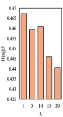
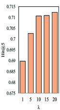
MovieLens	Gowalla

Figure 5. The $Hit@5$ scores of $\lambda$ varying experiments

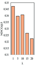
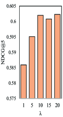
MovieLens	Gowalla

Figure 6. The $NDCG@5$ scores of $\lambda$ varying experiments

5.7.2. Effects of hyperparameter $L$

We study the influence of various slide window length $L$ from $\left\{4,5,6,7,8\right\}$ and show the results in Table 6. Apparently, setting $L$ too large or too small will both decrease the performance. Different from natural language sentences which always contain a key intention no matter how long the sentence is, we are not sure whether there is one or several intentions within a in sequence. A larger $L$ may introduce noises and give rise to the worse performance. Meanwhile, a smaller $L$ seems to ensure a single one intention but might damage the completeness of sequential patterns. Overall, $L=5$ is likely to be the optimal setting based on the results in Table 6.

Table 6. The effect of slide window length $L$.

Dataset	$L$	Hit@5	NDCG@5
MovieLens	$L$=4	0.4593	0.3414
	$L$=5	0.4672	0.3451
	$L$=6	0.4742	0.3550
	$L$=7	0.4695	0.3496
	$L$=8	0.4675	0.3441
Gowalla	$L$=4	0.6885	0.5849
	$L$=5	0.7124	0.6003
	$L$=6	0.7117	0.5997
	$L$=7	0.6832	0.5771
	$L$=8	0.6787	0.5751

6. Conclusion

In this paper, we propose a novel translation based architecture for context-aware sequential recommendation which captures the item-level and category-level transition patterns independently while maintaining the relations between these two sequences. To explore the subsidiary relationship between category and item, we further propose to adapt the variational auto-encoder to boosting the performance. Extensive experiments have been conducted over two datasets compared with several state-of-art methods. Results demonstrate the effectiveness of our proposed method by the superior performance over the state-of-the-art baselines.

References

- (1)
- Bahdanau et al. (2014) Dzmitry Bahdanau, Kyunghyun Cho, and Yoshua Bengio. 2014. Neural machine translation by jointly learning to align and translate. arXiv preprint arXiv:1409.0473 (2014).
- Bai et al. (2018) Ting Bai, Jian-Yun Nie, Wayne Xin Zhao, Yutao Zhu, Pan Du, and Ji-Rong Wen. 2018. An attribute-aware neural attentive model for next basket recommendation. In The 41st International ACM SIGIR Conference on Research & Development in Information Retrieval. ACM, 1201–1204.
- Chang et al. (2018) Buru Chang, Yonggyu Park, Donghyeon Park, Seongsoon Kim, and Jaewoo Kang. 2018. Content-Aware Hierarchical Point-of-Interest Embedding Model for Successive POI Recommendation.. In IJCAI. 3301–3307.
- Chen et al. (2019) Tong Chen, Hongzhi Yin, Hongxu Chen, Rui Yan, Quoc Viet Hung Nguyen, and Xue Li. 2019. AIR: Attentional Intention-Aware Recommender Systems. In 2019 IEEE 35th International Conference on Data Engineering (ICDE). IEEE, 304–315.
- Chen et al. (2018) Xu Chen, Hongteng Xu, Yongfeng Zhang, Jiaxi Tang, Yixin Cao, Zheng Qin, and Hongyuan Zha. 2018. Sequential recommendation with user memory networks. In Proceedings of the eleventh ACM international conference on web search and data mining. ACM, 108–116.
- Chen Ma and Liu (2019) Peng Kang Chen Ma and Xue Liu. 2019. Hierarchical Gating Networks for Sequential Recommendation. In Proceedings of the 25th ACM SIGKDD International Conference on Knowledge Discovery and Data Mining. ACM, 825–833.
- He et al. (2017a) Jing He, Xin Li, and Lejian Liao. 2017a. Category-aware Next Point-of-Interest Recommendation via Listwise Bayesian Personalized Ranking.. In IJCAI. 1837–1843.
- He et al. (2017b) Xiangnan He, Lizi Liao, Hanwang Zhang, Liqiang Nie, Xia Hu, and Tat-Seng Chua. 2017b. Neural collaborative filtering. In Proceedings of the 26th international conference on world wide web. International World Wide Web Conferences Steering Committee, 173–182.
- Hidasi et al. (2015) Balázs Hidasi, Alexandros Karatzoglou, Linas Baltrunas, and Domonkos Tikk. 2015. Session-based recommendations with recurrent neural networks. arXiv preprint arXiv:1511.06939 (2015).
- Higgins et al. (2017) Irina Higgins, Loic Matthey, Arka Pal, Christopher Burgess, Xavier Glorot, Matthew Botvinick, Shakir Mohamed, and Alexander Lerchner. 2017. beta-VAE: Learning Basic Visual Concepts with a Constrained Variational Framework. ICLR 2, 5 (2017), 6.
- Huang et al. (2018b) Jin Huang, Wayne Xin Zhao, Hongjian Dou, Ji-Rong Wen, and Edward Y Chang. 2018b. Improving sequential recommendation with knowledge-enhanced memory networks. In The 41st International ACM SIGIR Conference on Research & Development in Information Retrieval. ACM, 505–514.
- Huang et al. (2018a) Xiaowen Huang, Shengsheng Qian, Quan Fang, Jitao Sang, and Changsheng Xu. 2018a. CSAN: Contextual Self-Attention Network for User Sequential Recommendation. In 2018 ACM Multimedia Conference on Multimedia Conference. ACM, 447–455.
- Kang and McAuley (2018) Wang-Cheng Kang and Julian McAuley. 2018. Self-attentive sequential recommendation. In 2018 IEEE International Conference on Data Mining (ICDM). IEEE, 197–206.
- Kingma and Welling (2013) Diederik P Kingma and Max Welling. 2013. Auto-encoding variational bayes. arXiv preprint arXiv:1312.6114 (2013).
- Koren et al. (2009) Yehuda Koren, Robert Bell, and Chris Volinsky. 2009. Matrix factorization techniques for recommender systems. Computer 8 (2009), 30–37.
- LE et al. (2018) Duc Trong LE, Hady Wirawan LAUW, and Yuan Fang. 2018. Modeling contemporaneous basket sequences with twin networks for next-item recommendation. IJCAI.
- Li et al. (2018) Ranzhen Li, Yanyan Shen, and Yanmin Zhu. 2018. Next Point-of-Interest Recommendation with Temporal and Multi-level Context Attention. In 2018 IEEE International Conference on Data Mining (ICDM). IEEE, 1110–1115.
- Liang et al. (2018) Dawen Liang, Rahul G Krishnan, Matthew D Hoffman, and Tony Jebara. 2018. Variational autoencoders for collaborative filtering. In Proceedings of the 2018 World Wide Web Conference. International World Wide Web Conferences Steering Committee, 689–698.
- Liu et al. (2016b) Qiang Liu, Shu Wu, Diyi Wang, Zhaokang Li, and Liang Wang. 2016b. Context-aware sequential recommendation. In 2016 IEEE 16th International Conference on Data Mining (ICDM). IEEE, 1053–1058.
- Liu et al. (2016a) Qiang Liu, Shu Wu, Liang Wang, and Tieniu Tan. 2016a. Predicting the next location: A recurrent model with spatial and temporal contexts. In Thirtieth AAAI Conference on Artificial Intelligence.
- Luong et al. (2015) Minh-Thang Luong, Hieu Pham, and Christopher D Manning. 2015. Effective approaches to attention-based neural machine translation. arXiv preprint arXiv:1508.04025 (2015).
- Rakkappan and Rajan (2019) Lakshmanan Rakkappan and Vaibhav Rajan. 2019. Context-Aware Sequential Recommendations withStacked Recurrent Neural Networks. In The World Wide Web Conference. ACM, 3172–3178.
- Rendle et al. (2009) Steffen Rendle, Christoph Freudenthaler, Zeno Gantner, and Lars Schmidt-Thieme. 2009. BPR: Bayesian personalized ranking from implicit feedback. In Proceedings of the twenty-fifth conference on uncertainty in artificial intelligence. AUAI Press, 452–461.
- Rendle et al. (2010) Steffen Rendle, Christoph Freudenthaler, and Lars Schmidt-Thieme. 2010. Factorizing personalized markov chains for next-basket recommendation. In Proceedings of the 19th international conference on World wide web. ACM, 811–820.
- Sachdeva et al. (2019) Noveen Sachdeva, Giuseppe Manco, Ettore Ritacco, and Vikram Pudi. 2019. Sequential Variational Autoencoders for Collaborative Filtering. In Proceedings of the Twelfth ACM International Conference on Web Search and Data Mining. ACM, 600–608.
- Sennrich et al. (2015) Rico Sennrich, Barry Haddow, and Alexandra Birch. 2015. Improving neural machine translation models with monolingual data. arXiv preprint arXiv:1511.06709 (2015).
- Sutskever et al. (2014) Ilya Sutskever, Oriol Vinyals, and Quoc V Le. 2014. Sequence to sequence learning with neural networks. In Advances in neural information processing systems. 3104–3112.
- Tang and Wang (2018) Jiaxi Tang and Ke Wang. 2018. Personalized top-n sequential recommendation via convolutional sequence embedding. In Proceedings of the Eleventh ACM International Conference on Web Search and Data Mining. ACM, 565–573.
- Vaswani et al. (2017) Ashish Vaswani, Noam Shazeer, Niki Parmar, Jakob Uszkoreit, Llion Jones, Aidan N Gomez, Łukasz Kaiser, and Illia Polosukhin. 2017. Attention is all you need. In Advances in neural information processing systems. 5998–6008.
- Wang et al. (2015) Pengfei Wang, Jiafeng Guo, Yanyan Lan, Jun Xu, Shengxian Wan, and Xueqi Cheng. 2015. Learning hierarchical representation model for nextbasket recommendation. In Proceedings of the 38th International ACM SIGIR conference on Research and Development in Information Retrieval. ACM, 403–412.
- Yang et al. (2017) Carl Yang, Lanxiao Bai, Chao Zhang, Quan Yuan, and Jiawei Han. 2017. Bridging collaborative filtering and semi-supervised learning: a neural approach for poi recommendation. In Proceedings of the 23rd ACM SIGKDD International Conference on Knowledge Discovery and Data Mining. ACM, 1245–1254.
- Yao et al. (2017) Di Yao, Chao Zhang, Jianhui Huang, and Jingping Bi. 2017. Serm: A recurrent model for next location prediction in semantic trajectories. In Proceedings of the 2017 ACM on Conference on Information and Knowledge Management. ACM, 2411–2414.
- Yu et al. (2016) Feng Yu, Qiang Liu, Shu Wu, Liang Wang, and Tieniu Tan. 2016. A dynamic recurrent model for next basket recommendation. In Proceedings of the 39th International ACM SIGIR conference on Research and Development in Information Retrieval. ACM, 729–732.
- Zhang et al. (2016) Biao Zhang, Deyi Xiong, Jinsong Su, Hong Duan, and Min Zhang. 2016. Variational neural machine translation. arXiv preprint arXiv:1605.07869 (2016).
- Zhang et al. (2019) Shuai Zhang, Yi Tay, Lina Yao, Aixin Sun, and Jake An. 2019. Next Item Recommendation with Self-Attentive Metric Learning. In Thirty-Third AAAI Conference on Artificial Intelligence, Vol. 9.
- Zhou et al. (2018) Chang Zhou, Jinze Bai, Junshuai Song, Xiaofei Liu, Zhengchao Zhao, Xiusi Chen, and Jun Gao. 2018. ATRank: An attention-based user behavior modeling framework for recommendation. In Thirty-Second AAAI Conference on Artificial Intelligence.