Sensor-Independent Illumination Estimation for DNN Models

Abstract

While modern deep neural networks (DNNs) achieve state-of-the-art results for illuminant estimation, it is currently necessary to train a separate DNN for each type of camera sensor. This means when a camera manufacturer uses a new sensor, it is necessary to retrain an existing DNN model with training images captured by the new sensor. This paper addresses this problem by introducing a novel sensor-independent illuminant estimation framework. Our method learns a sensor-independent working space that can be used to canonicalize the RGB values of any arbitrary camera sensor. Our learned space retains the linear property of the original sensor raw-RGB space and allows unseen camera sensors to be used on a single DNN model trained on this working space. We demonstrate the effectiveness of this approach on several different camera sensors and show it provides performance on par with state-of-the-art methods that were trained per sensor.

1 Introduction and Motivation

Color constancy is the constant appearance of object colors under different illumination conditions [Foster(2003)]. Human vision has this illumination adaption ability to recognize the same object colors under different scene lighting [Maloney(1999)]. Camera sensors, however, do not have this ability and as a result, computational color constancy is required to be applied onboard the camera. In a photography context, this procedure is typically termed white balance. The key challenge for computational color constancy is the ability to estimate a camera sensor’s RGB response to the scene’s illumination. Illumination estimation, or auto white balance (AWB), is a fundamental procedure applied onboard all cameras and is critical in ensuring the correct interpretation of scene colors.

Computational color constancy can be described in terms of the physical image formation process as follows. Let $\mathbf{I}=\{\mathbf{I}_{r},\mathbf{I}_{g},\mathbf{I}_{b}\}$ denote an image captured in the linear raw-RGB space. The value of each color channel $c=\{\text{R},\text{G},\text{B}\}$ for a pixel located at $x$ in $\mathbf{I}$ is given by the following equation [Basri and Jacobs(2003)]:

$$\mathbf{I}_{c}(x)=\int_{\gamma}\rho(x,\lambda)R(x,\lambda)S_{c}(\lambda)d\lambda,$$ (1)

where $\gamma$ is the visible light spectrum (approximately 380nm to 780nm), $\rho(\cdot)$ is the illuminant spectral power distribution, $R(\cdot)$ is the captured scene’s spectral reflectance properties, and $S(\cdot)$ is the camera sensor response function at wavelength $\lambda$. The problem can be simplified by assuming a single uniform illuminant in the scene as follows:

$$\mathbf{I}_{c}=\boldsymbol{\ell}_{c}\!\times\!\mathbf{R}_{c},$$ (2)

where $\boldsymbol{\ell}_{c}$ is the scene illuminant value of color channel $c$. A standard approach to this problem is to use a linear model (i.e., a $3\!\times\!3$ diagonal matrix) such that $\boldsymbol{\ell}_{\text{R}}=\boldsymbol{\ell}_{\text{G}}=\boldsymbol{\ell}_{\text{B}}$ (i.e., white illuminant).

Typically, $\boldsymbol{\ell}$ is unknown and should be defined to obtain the true objects’ body reflectance values $\mathbf{R}$ in the input image $\mathbf{I}$. The value of $\boldsymbol{\ell}$ is specific to the camera sensor response function $S(\cdot)$, meaning that the same scene captured by different camera sensors results in different values of $\boldsymbol{\ell}$. Fig. 1 shows an example.

Illuminant estimation methods aim to estimate the value $\boldsymbol{\ell}$ from the sensor’s raw-RGB image. Recently, deep neural network (DNN) methods have demonstrated state-of-the-art results for the illuminant estimation task. These approaches, however, need to train the DNN model per camera sensor. This is a significant drawback. When a camera manufacturer decides to use a new sensor, the DNN model will need to be retrained on a new image dataset captured by the new sensor. Collecting such datasets with the corresponding ground-truth illuminant raw-RGB values is a tedious process. As a result, many AWB algorithms deployed on cameras still rely on simple statistical-based methods even though the accuracy is not comparable to those obtained by the learning-based methods [Afifi et al.(2019b)Afifi, Punnappurath, Finlayson, and Brown].

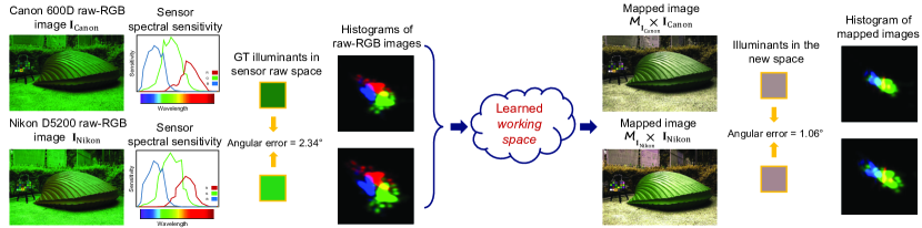
Figure 1: A scene captured by two different camera sensors results in different ground truth illuminants due to different camera sensor responses. We learn a device-independent working space that reduces the difference between ground truth illuminants of the same scenes.

Contribution

In this paper, we introduce a sensor-independent learning framework for illuminant estimation. The idea is similar to the color space conversion process applied onboard cameras that maps the sensor-specific RGB values to a perceptual-based color space – namely, CIE XYZ. The color space conversion process estimates a color space transform (CST) matrix to map white-balanced sensor-specific raw-RGB images to CIE XYZ [Ramanath et al.(2005)Ramanath, Snyder, Yoo, and Drew, Karaimer and Brown(2016)]. This process is applied onboard cameras after the illuminant estimation and white-balance step, and relies on the estimated scene illuminant to compute the CST matrix [Can Karaimer and Brown(2018)]. Our solution, however, is to learn a new space that is used before the illuminant estimation step. Specifically, we design a novel unsupervised deep learning framework that learns how to map each input image, captured by arbitrary camera sensor, to a non-perceptual sensor-independent working space. Mapping input images to this space allows us to train our model using training sets captured by different camera sensors, achieving good accuracy and generalizing well for unseen camera sensors, as shown in Fig. 2.

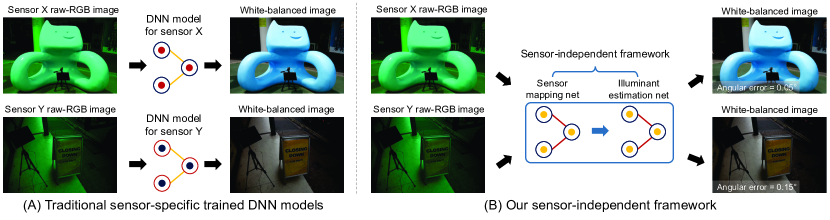
Figure 2: (A) Traditional learning-based illuminant estimation methods train or fine-tune a model per camera sensor. (B) Our method can be trained on images captured by different camera sensors and generalizes well for unseen camera sensors. Shown images are rendered in the sRGB color space by the camera imaging pipeline in [Karaimer and Brown(2016)] to aid visualization.

2 Related Work

We discuss two areas of related work: (i) illumination estimation and (ii) mapping camera sensor responses.

2.1 Illumination Estimation

As previously discussed, illuminant estimation is the key routine that makes up a camera’s AWB function. Illuminant estimation methods aim to estimate the illumination in the imaged scene directly from a raw-RGB image without a known achromatic reference scene patch. We categorize the illuminant estimation methods into two categories, which are: (i) sensor-independent methods and (ii) sensor-dependent methods.

Sensor-Independent Methods

These methods operate using statistics from an image’s color distribution and spatial layout to estimate the scene illuminant. Representative statistical-based methods include: Gray-World [Buchsbaum(1980)], White-Patch [Brainard and Wandell(1986)], Shades-of-Gray [Finlayson and Trezzi(2004)], Gray-Edges, and PCA-based Bright-and-Dark Colors [Cheng et al.(2014)Cheng, Prasad, and Brown]. These methods are fast and easy to implement; however, their results are not always satisfactory.

Sensor-Dependent Methods

Learning-based models outperform statistical-based methods by training sensor-specific models on training examples provided with the labeled images with ground-truth illumination obtained from physical charts placed in the scene with achromatic reference patches. These training images are captured with the sensor make and model being trained. Representative examples include Bayesian-based methods [Brainard and Freeman(1997), Rosenberg et al.(2004)Rosenberg, Ladsariya, and Minka, Gehler et al.(2008)Gehler, Rother, Blake, Minka, and Sharp], gamut-based methods [Forsyth(1990), Finlayson et al.(2006)Finlayson, Hordley, and Tastl, Gijsenij et al.(2010)Gijsenij, Gevers, and Van De Weijer], exemplar-based methods [Gijsenij and Gevers(2011), Joze and Drew(2014), Banic and Loncaric(2015)], bias-correction methods [Finlayson(2013), Finlayson(2018), Afifi et al.(2019b)Afifi, Punnappurath, Finlayson, and Brown], and, more recently, DNN methods [Lou et al.(2015)Lou, Gevers, Hu, Lucassen, et al., Barron(2015), Oh and Kim(2017), Shi et al.(2016)Shi, Loy, and Tang, Hu et al.(2017)Hu, Wang, and Lin, Barron and Tsai(2017)], including few-shot learning [McDonagh et al.(2018)McDonagh, Parisot, Li, and Slabaugh]. The obvious drawback of these methods is that they do not generalize well for arbitrary camera sensors without retraining/fine-tuning on samples captured by testing camera sensor. Our learning method, however, is explicitly designed to be sensor-independent and generalizes well for unseen camera sensors without the need to retrain/tune our model.

2.2 Mapping Camera Sensor Responses

Another research topic related to our work is mapping camera raw-RGB sensor responses to a perceptual color space. This process is applied onboard digital cameras to map the captured sensor-specific raw-RGB image to a standard device-independent “canonical” space (e.g., CIE XYZ) [Ramanath et al.(2005)Ramanath, Snyder, Yoo, and Drew, Karaimer and Brown(2016)]. Usually this conversion is performed using a $3\!\times\!3$ matrix and requires an accurate estimation of the scene illuminant [Can Karaimer and Brown(2018)]. It is important to note that this mapping to CIE XYZ requires that white-balance procedure first be applied. As a result, it is not possible to use CIE XYZ as the canonical color space to perform illumination estimation.

Work by Nguyen et al. [Nguyen et al.(2014)Nguyen, Prasad, and Brown] studied several transformations to map responses from a source camera sensor to a target camera sensor, instead of mapping to a perceptual space. In their study, a color rendition reference chart is captured by both source and target camera sensors in order to compute the raw-to-raw mapping function. Learning a mapping transformation between responses of two different sensors is also adapted in [Gao et al.(2017)Gao, Zhang, Li, and Li]. While our approach is similar in this goal, the work in [Nguyen et al.(2014)Nguyen, Prasad, and Brown, Gao et al.(2017)Gao, Zhang, Li, and Li] has no mechanism to map an unseen sensor to a canonical working space without explicit calibration.

3 Proposed Method

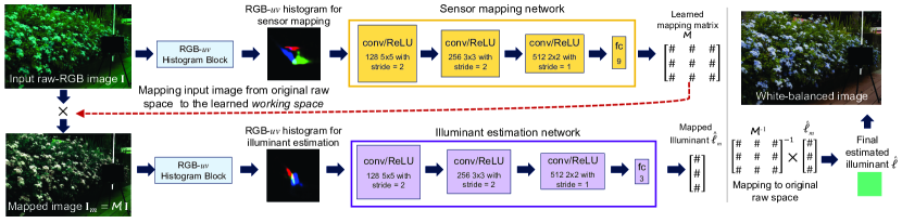
Figure 3: Our proposed method consists of two networks: (i) a sensor mapping network and (ii) an illuminant estimation network. Our networks are trained jointly in an end-to-end manner to learn an image-specific mapping matrix (resulting from the sensor mapping network) and scene illuminant in the learned space (resulting from the illuminant estimation network). The final estimated illuminant is produced by mapping the result illuminant from our learned space to the input image’s camera-specific raw space.

Fig. 3 provides an overview of our framework. Our method accepts thumbnail ($150\!\times\!150$ pixels) linear raw-RGB images, captured by an arbitrary camera sensor, and estimates scene illuminant RGB vectors in the same space of input images.

We rely on color distribution of input thumbnail image $\mathbf{I}$ to estimate an image-specific transformation matrix that maps the input image to our working space. This mapping allows us to accept images captured by different sensors and estimate scene illuminant values in the original space of input images.

We begin with the formulation of our problem followed by a detailed description of our framework components and the training process. Note that we will assume input raw-RGB images are represented as $3\!\times\!n$ matrices, where $n=150\!\times\!150$ is the total number of pixels in the thumbnail image and the three rows represent the R, G, and B values.

3.1 Problem Formulation

We propose to work in a new learned space for illumination estimation. This space is sensor-independent and retains the linear property of the original raw-RGB space. To that end, we introduce a learnable $3\!\times\!3$ matrix $\boldsymbol{\mathcal{M}}$ that maps an input image $\mathbf{I}$ from its original sensor-specific space to a new working space. We can reformulate Eq. 2 as follows:

$$\boldsymbol{\mathcal{M}}^{-1}\boldsymbol{\mathcal{M}}\mathbf{I}=\texttt{diag}(\boldsymbol{\mathcal{M}}^{-1}\boldsymbol{\mathcal{M}}\boldsymbol{\ell})\mathbf{R},$$ (3)

where $\texttt{diag}(\cdot)$ is a diagonal matrix and $\boldsymbol{\mathcal{M}}$ is a learned matrix that maps arbitrary sensor responses to a sensor-independent space.

Given a mapped image $\mathbf{I}_{m}=\boldsymbol{\mathcal{M}}\mathbf{I}$ in our learned space, we aim to estimate the mapped vector $\boldsymbol{\ell}_{m}=\boldsymbol{\mathcal{M}}\boldsymbol{\ell}$ that represents the scene illumination values of $\mathbf{I}_{m}$ in the new space. The original scene illuminant (represented in the original sensor raw-RGB space) can be reconstructed by the following equation:

$$\boldsymbol{\ell}=\boldsymbol{\mathcal{M}}^{-1}\boldsymbol{\ell}_{m}.$$ (4)

3.2 RGB–$uv$ Histogram Block

Prior work has shown that the illumination estimation problem is related primarily to the image’s color distribution [Cheng et al.(2014)Cheng, Prasad, and Brown, Barron(2015)]. Accordingly, we use the image’s color distribution as an input for our method. Representing the image using a full 3D RGB histogram requires significant amounts of memory – for example, a $256^{3}$ RGB histogram requires more than 16 million entries. Down-sampling the histogram – for example, to 64-bins – still requires a considerable amount of memory.

Our method relies on the RGB-$uv$ histogram feature used in [Afifi et al.(2019a)Afifi, Price, Cohen, and Brown]. This feature represents the image color distribution in the log of chromaticity space [Drew et al.(2003)Drew, Finlayson, and Hordley]. Unlike the original RGB-$uv$ feature, we use two learnable parameters to control the contribution of each color channel in the generated histogram and the smoothness of histogram bins. Specifically, the RGB-$uv$ histogram block represents the color distribution of an image $\mathbf{I}$ as a three-layer histogram $\mathbf{H}(\mathbf{I})$ represented as an $m\!\times\!m\!\times 3$ tensor. The produced histogram $\mathbf{H}(\mathbf{I})$ is parameterized by $uv$ and computed as follows:

$$\begin{gathered}\mathbf{I}_{y}(i)=\sqrt{\mathbf{I}_{\textrm{R}(i)}^{2}+\mathbf{I}_{\textrm{G}(i)}^{2}+\mathbf{I}_{\textrm{B}(i)}^{2}},\\ \mathbf{I}_{u1(i)}=\log{\left(\frac{\mathbf{I}_{\textrm{R}(i)}}{\mathbf{I}_{\textrm{G}(i)}}+\epsilon\right)}\textrm{ , }\mathbf{I}_{v1(i)}=\log{\left(\frac{\mathbf{I}_{\textrm{R}(i)}}{\mathbf{I}_{\textrm{B}(i)}}+\epsilon\right)},\\ \mathbf{I}_{u2(i)}=\log{\left(\frac{\mathbf{I}_{\textrm{G}(i)}}{\mathbf{I}_{\textrm{R}(i)}}+\epsilon\right)}\textrm{ , }\mathbf{I}_{v2(i)}=\log{\left(\frac{\mathbf{I}_{\textrm{G}(i)}}{\mathbf{I}_{\textrm{B}(i)}}+\epsilon\right)},\\ \mathbf{I}_{u3(i)}=\log{\left(\frac{\mathbf{I}_{\textrm{B}(i)}}{\mathbf{I}_{\textrm{R}(i)}}+\epsilon\right)}\textrm{ , }\mathbf{I}_{v3(i)}=\log{\left(\frac{\mathbf{I}_{\textrm{B}(i)}}{\mathbf{I}_{\textrm{G}(i)}}+\epsilon\right)},\\ \mathbf{H}\left(\mathbf{I}\right)_{(u,v,c)}=\left(s_{c}\sum_{i}\mathbf{I}_{y(i)}\exp{\left(-\left|\mathbf{I}_{uc(i)}-u\right|/\sigma_{c}^{2}\right)}\exp{\left(-\left|\mathbf{I}_{vc(i)}-v\right|/\sigma_{c}^{2}\right)}\right)^{1/2},\end{gathered}$$ (5)

where $i=\{1,...,n\}$, $c\in{\{1,2,3\}}$ represents each color channel in $\mathbf{H}$, $\epsilon$ is a small positive constant added for numerical stability, and $s_{c}$ and $\sigma_{c}$ are learnable scale and fall-off parameters, respectively. The scale factor $s_{c}$ controls the contribution of each layer in our histogram, while the fall-off factor $\sigma_{c}$ controls the smoothness of the histogram’s bins of each layer. The values of these parameters (i.e., $s_{c}$ and $\sigma_{c}$) are learned during the training phase.

3.3 Network Architecture

As shown in Fig. 3, our framework consists of two networks: (i) a sensor mapping network and (ii) an illuminant estimation network. The input to each network is the RGB-$uv$ histogram feature produced by our histogram block. The sensor mapping network accepts an RGB-$uv$ histogram of a thumbnail raw-RGB image $\mathbf{I}$ in its original sensor space, while the illuminant estimation network accepts RGB-$uv$ histograms of the mapped image $\mathbf{I}_{m}$ to our learned space. In our implementation, we use $m=61$ and each histogram feature is represented by a $61\!\times\!61\!\times\!3$ tensor.

We use a simple network architecture for each network. Specifically, each network consists of three conv/ReLU layers followed by a fully connected (fc) layer. The kernel size and stride step used in each conv layer are shown in Fig. 3.

In the sensor mapping network, the last fc layer has nine neurons. The output vector $\boldsymbol{v}$ of this fc layer is reshaped to construct a $3\!\times\!3$ matrix $\boldsymbol{V}$, which is used to build $\boldsymbol{\mathcal{M}}$ as described in the following equation:

$$\boldsymbol{\mathcal{M}}=\frac{1}{\lVert\boldsymbol{V}\rVert_{1}+\epsilon}\left|\boldsymbol{V}\right|,$$ (6)

where $\left|\cdot\right|$ is the modulus (absolute magnitude), $\lVert\cdot\rVert_{1}$ is the matrix 1-norm, and $\epsilon$ is added for numerical stability. The modulus step is necessary to avoid negative values in the mapped image $\mathbf{I}_{m}$, while the normalization step is used to avoid having extremely large values in $\mathbf{I}_{m}$. Note the values of $\boldsymbol{\mathcal{M}}$ are image-specific, meaning that its values are produced based on the input image’s color distribution in the original raw-RGB space.

There are three neurons in the last fc layer of the illuminant estimation network to produce illuminant vector $\hat{\boldsymbol{\ell}}_{m}$ of the mapped image $\mathbf{I}_{m}$. Note that the estimated vector $\hat{\boldsymbol{\ell}}_{m}$ represents the scene illuminant in our learned space. The final result is obtained by mapping $\hat{\boldsymbol{\ell}}_{m}$ back to the original space of $\mathbf{I}$ using Eq. 4.

3.4 Training

We jointly train our sensor mapping and illuminant estimation networks in an end-to-end manner using the adaptive moment estimation (Adam) optimizer [Kingma and Ba(2014)] with a decay rate of gradient moving average $\beta_{1}=0.85$, a decay rate of squared gradient moving average $\beta_{2}=0.99$, and a mini-batch with eight observations at each iteration. We initialized both network weights with Xavier initialization [Glorot and Bengio(2010)]. The learning rate was set to $10^{-5}$ and decayed every five epochs.

We adopt the recovery angular error (referred to as the angular error) as our loss function [Finlayson et al.(1995)Finlayson, Funt, and Barnard]. The angular error is computed between the ground truth illuminant $\boldsymbol{\ell}$ and our estimated illuminant $\hat{\boldsymbol{\ell}}_{m}$ after mapping it to the original raw-RGB space of training image $\mathbf{I}$. The loss function can be described by the following equation:

$$L(\hat{\boldsymbol{\ell}}_{m},\boldsymbol{\mathcal{M}})=\cos^{-1}\left(\frac{\boldsymbol{\ell}\cdot\left(\boldsymbol{\mathcal{M}}^{-1}\hat{\boldsymbol{\ell}}_{m}\right)}{\lVert\boldsymbol{\ell}\rVert\lVert\boldsymbol{\mathcal{M}}^{-1}\hat{\boldsymbol{\ell}}_{m}\rVert}\right),$$ (7)

where $\lVert\cdot\rVert$ is the Euclidean norm, and ($\cdot$) is the vector dot-product.

As the values of $\boldsymbol{\mathcal{M}}$ are produced by the sensor mapping network, there is a possibility of producing a singular matrix output. In this case, we add small offset $\mathcal{N}(0,1)\!\times\!10^{-4}$ to each parameter in $\boldsymbol{\mathcal{M}}$ to make it invertible.

At the end of the training process, our framework learns an image-specific matrix $\boldsymbol{\mathcal{M}}$ that maps an input image taken by an arbitrary sensor to the learned space. Fig. 4 shows an example of three different camera responses capturing the same set of scenes. As shown in Fig. 4-(A), the estimated illuminants of these sensors are bounded in the learned space. These illuminants are mapped back to the original raw-RGB sensor space of the corresponding input images using Eq. 4. As shown in Fig. 4-(B) and Fig. 4-(C), our final estimated illuminants are close to the ground truth illuminants of each camera sensor.

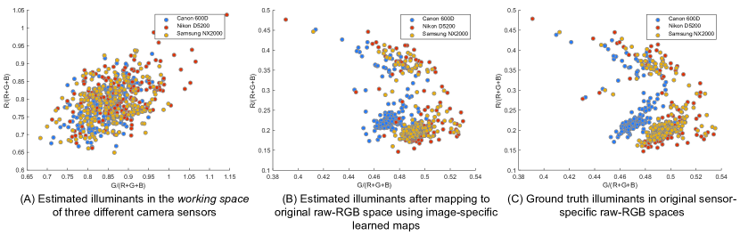
Figure 4: Raw-RGB images capture the same set of scenes using three different cameras taken from the NUS 8-Cameras dataset [Cheng et al.(2014)Cheng, Prasad, and Brown]. (A) Estimated illuminants resulted from the illuminant estimation network in our learned working space. (B) Estimated illuminants after mapping to the original raw-RGB space. This mapping is performed by multiplying each illuminant vector by the inverse of the learned image-specific mapping matrix (resulting from the sensor mapping network). (C) Corresponding ground truth illuminants in the original raw-RGB space of each image.

4 Experimental Results

Table 1: Angular errors on the NUS 8-Cameras [Cheng et al.(2014)Cheng, Prasad, and Brown] and Gehler-Shi [Gehler et al.(2008)Gehler, Rother, Blake, Minka, and Sharp] datasets. Methods highlighted in gray are trained/tuned for each camera sensor (i.e., sensor-specific models). The lowest errors are highlighted in yellow.

NUS 8-Cameras Dataset Method	Mean	Med.	Best 25%	Worst 25%
White-Patch [Brainard and Wandell(1986)]	9.91	7.44	1.44	21.27
Pixel-based Gamut [Gijsenij et al.(2010)Gijsenij, Gevers, and Van De Weijer]	5.27	4.26	1.28	11.16
Grey-world (GW) [Buchsbaum(1980)]	4.59	3.46	1.16	9.85
Edge-based Gamut [Gijsenij et al.(2010)Gijsenij, Gevers, and Van De Weijer]	4.40	3.30	0.99	9.83
Shades-of-Gray [Finlayson and Trezzi(2004)]	3.67	2.94	0.98	7.75
[HTML]EFEFEFBayesian [Gehler et al.(2008)Gehler, Rother, Blake, Minka, and Sharp]	3.50	2.36	0.78	8.02
Local Surface Reflectance [Gao et al.(2014)Gao, Han, Yang, Li, and Li]	3.45	2.51	0.98	7.32
2nd-order Gray-Edge [Van De Weijer et al.(2007)Van De Weijer, Gevers, and Gijsenij]	3.36	2.70	0.89	7.14
1st-order Gray-Edge [Van De Weijer et al.(2007)Van De Weijer, Gevers, and Gijsenij]	3.35	2.58	0.79	7.18
Quasi-unsupervised [Bianco and Cusano(2019)]	3.00	2.25	-	-
[HTML]EFEFEFCorrected-Moment [Finlayson(2013)]	2.95	2.05	0.59	6.89
PCA-based B/W Colors [Cheng et al.(2014)Cheng, Prasad, and Brown]	2.93	2.33	0.78	6.13
Grayness Index [Qian et al.(2019)Qian, Nikkanen, Kämäräinen, and Matas]	2.91	1.97	0.56	6.67
[HTML]EFEFEFColor Dog [Banic and Loncaric(2015)]	2.83	1.77	0.48	7.04
[HTML]EFEFEFAPAP using GW [Afifi et al.(2019b)Afifi, Punnappurath, Finlayson, and Brown]	2.40	1.76	0.55	5.42
[HTML]EFEFEFConv Color Constancy [Barron(2015)]	2.38	1.69	0.45	5.85
[HTML]EFEFEFEffective Regression Tree [Cheng et al.(2015)Cheng, Price, Cohen, and Brown]	2.36	1.59	0.49	5.54
[HTML]EFEFEFWB-sRGB (modified for raw-RGB) [Afifi et al.(2019a)Afifi, Price, Cohen, and Brown]	2.26	1.60	0.48	5.21
[HTML]EFEFEFDeep Specialized Net [Shi et al.(2016)Shi, Loy, and Tang]	2.24	1.46	0.48	6.08
[HTML]EFEFEFMeta-AWB w 20 tuning images [McDonagh et al.(2018)McDonagh, Parisot, Li, and Slabaugh]	2.23	1.49	0.49	5.20
[HTML]EFEFEFSqueezeNet-FC4	2.23	1.57	0.47	5.15
[HTML]EFEFEFAlexNet-FC4 [Hu et al.(2017)Hu, Wang, and Lin]	2.12	1.53	0.48	4.78
[HTML]EFEFEFFast Fourier – thumb, 2 channels [Barron and Tsai(2017)]	2.06	1.39	0.39	4.80
[HTML]EFEFEFFast Fourier – full, 4 channels [Barron and Tsai(2017)]	1.99	[HTML]FFFC9E1.31	[HTML]FFFC9E0.35	4.75
[HTML]EFEFEFQuasi-unsupervised (tuned) [Bianco and Cusano(2019)]	[HTML]FFFC9E1.97	1.41	-	-
Avg. result for sensor-independent	4.26	3.25	0.99	9.43
Avg. result for sensor-dependent	2.40	1.64	0.50	5.75
Sensor-independent (Ours)	2.05	1.50	0.52	[HTML]FFFC9E4.48

Gehler-Shi Dataset Method	Mean	Med.	Best 25%	Worst 25%
White-Patch [Brainard and Wandell(1986)]	7.55	5.68	1.45	16.12
Edge-based Gamut [Gijsenij et al.(2010)Gijsenij, Gevers, and Van De Weijer]	6.52	5.04	5.43	13.58
Grey-world (GW) [Buchsbaum(1980)]	6.36	6.28	2.33	10.58
1st-order Gray-Edge [Van De Weijer et al.(2007)Van De Weijer, Gevers, and Gijsenij]	5.33	4.52	1.86	10.03
2nd-order Gray-Edge [Van De Weijer et al.(2007)Van De Weijer, Gevers, and Gijsenij]	5.13	4.44	2.11	9.26
Shades-of-Gray [Finlayson and Trezzi(2004)]	4.93	4.01	1.14	10.20
[HTML]EFEFEFBayesian [Gehler et al.(2008)Gehler, Rother, Blake, Minka, and Sharp]	4.82	3.46	1.26	10.49
[HTML]EFEFEFPixels-based Gamut [Gijsenij et al.(2010)Gijsenij, Gevers, and Van De Weijer]	4.20	2.33	0.50	10.72
Quasi-unsupervised [Bianco and Cusano(2019)]	3.46	2.23	-	-
PCA-based B/W Colors [Cheng et al.(2014)Cheng, Prasad, and Brown]	3.52	2.14	0.50	8.74
[HTML]EFEFEFNetColorChecker [Lou et al.(2015)Lou, Gevers, Hu, Lucassen, et al.]	3.10	2.30	-	-
Grayness Index [Qian et al.(2019)Qian, Nikkanen, Kämäräinen, and Matas]	3.07	1.87	0.43	7.62
[HTML]EFEFEFMeta-AWB w 20 tuning images [McDonagh et al.(2018)McDonagh, Parisot, Li, and Slabaugh]	3.00	2.02	0.58	7.17
[HTML]EFEFEFQuasi-unsupervised [Bianco and Cusano(2019)] (tuned)	2.91	1.98	-	-
[HTML]EFEFEFCorrected-Moment [Finlayson(2013)]	2.86	2.04	0.70	6.34
[HTML]EFEFEFAPAP using GW [Afifi et al.(2019b)Afifi, Punnappurath, Finlayson, and Brown]	2.76	2.02	0.53	6.21
[HTML]EFEFEFBianco et al.’s CNN [Bianco et al.(2015)Bianco, Cusano, and Schettini]	2.63	1.98	0.72	3.90
[HTML]EFEFEFEffective Regression Tree [Cheng et al.(2015)Cheng, Price, Cohen, and Brown]	2.42	1.65	0.38	5.87
[HTML]EFEFEFWB-sRGB (modified for raw-RGB) [Afifi et al.(2019a)Afifi, Price, Cohen, and Brown]	2.07	1.38	[HTML]FFFC9E0.29	5.11
[HTML]EFEFEFFast Fourier - thumb, 2 channels [Barron and Tsai(2017)]	2.01	1.13	0.30	5.14
[HTML]EFEFEFConv Color Constancy [Barron(2015)]	1.95	1.22	0.35	4.76
[HTML]EFEFEFDeep Specialized Net [Shi et al.(2016)Shi, Loy, and Tang]	1.90	1.12	0.31	4.84
[HTML]EFEFEFFast Fourier - full, 4 channels [Barron and Tsai(2017)]	1.78	[HTML]FFFC9E0.96	[HTML]FFFC9E0.29	4.62
[HTML]EFEFEFAlexNet-FC4 [Hu et al.(2017)Hu, Wang, and Lin]	1.77	1.11	0.34	4.29
[HTML]EFEFEFSqueezeNet-FC4 [Hu et al.(2017)Hu, Wang, and Lin]	[HTML]FFFC9E1.65	1.18	0.38	[HTML]FFFC9E3.78
Avg. result for sensor-independent	5.10	4.03	1.91	10.77
Avg. result for sensor-dependent	2.62	1.75	0.50	5.95
Sensor-independent (Ours)	2.77	1.93	0.55	6.53

In our experiments, we used all cameras of three different datasets, which are: (i) NUS 8-Camera [Cheng et al.(2014)Cheng, Prasad, and Brown], (ii) Gehler-Shi [Gehler et al.(2008)Gehler, Rother, Blake, Minka, and Sharp], and (iii) Cube+ [Banić and Lončarić(2017)] datasets. In total, we have 4,014 raw-RGB images captured by 11 different camera sensors.

We followed the leave-one-out cross-validation scheme to evaluate our method. Specifically, we excluded all images captured by one camera for testing and trained a model with the remaining images. This process was repeated for all cameras. We also tested our method on the Cube dataset. In this experiment, we used a trained model on images from the NUS and Gehler-Shi datasets, and excluded all images from the Cube+ dataset. The calibration objects (i.e., X-Rite color chart or SpyderCUBE) were masked out in both training and testing processes.

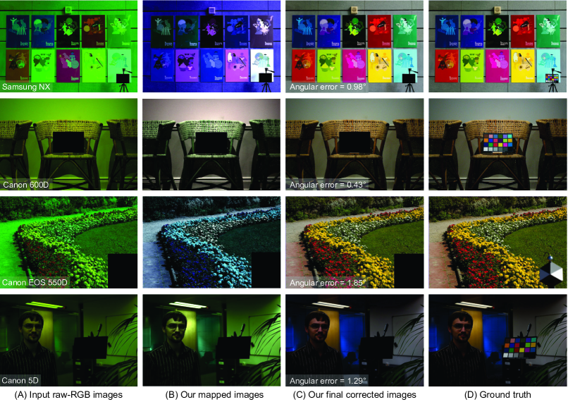
Figure 5: Qualitative results of our method. (A) Input raw-RGB images. (B) After mapping images in (A) to the learned space. (C) After correcting images in (A) based on our estimated illuminants. (D) Corrected by ground truth illuminants. Shown images are rendered in the sRGB color space by the camera imaging pipeline in [Karaimer and Brown(2016)] to aid visualization.

Unlike results reported by existing learning methods which use three-fold cross-validation for evaluation, our reported results were obtained by models that were not trained on any example of the testing camera sensor.

In Tables 1–2, the mean, median, best 25%, and the worst 25% of the angular error between our estimated illuminants and ground truth are reported. The best 25% and worst 25% are the mean of the smallest 25% angular error values and the mean of the highest 25% angular error values, respectively. We highlight learning methods (i.e., models trained/tuned for the testing sensor) with gray in the shown tables. The reported results are taken from previous papers, except for the recent work in [Afifi et al.(2019a)Afifi, Price, Cohen, and Brown], which was proposed for white balancing images saved in the sRGB color space. We modified [Afifi et al.(2019a)Afifi, Price, Cohen, and Brown] to work in the raw-RGB space by replacing the training polynomial matrices with the ground truth illuminant vectors. The shown results of [Afifi et al.(2019a)Afifi, Price, Cohen, and Brown] were obtained by using training data from a single camera sensor (i.e., sensor-specific) with the following settings: $k=15$, $\sigma=0.45$, $m=91$, and $c=191$. For the recent work in [Bianco and Cusano(2019)], we include results of the unsupervised and tuned models. Our method performs better than all statistical-based methods and outperforms some sensor-specific learning methods. We obtain results on par with the sensor-specific state-of-the-art results in the NUS 8-Camera dataset (Table 1).

Table 2: Angular errors on the Cube and Cube+ datasets [Banić and Lončarić(2017)]. Methods highlighted in gray are trained/tuned for each camera sensor (i.e., sensor-specific models). The lowest errors are highlighted in yellow.

Cube Dataset Method	Mean	Med.	Best 25%	Worst 25%
White-Patch [Brainard and Wandell(1986)]	6.58	4.48	1.18	15.23
Grey-world (GW) [Buchsbaum(1980)]	3.75	2.91	0.69	8.18
Shades-of-Gray [Finlayson and Trezzi(2004)]	2.58	1.79	0.38	6.19
2nd-order Gray-Edge [Van De Weijer et al.(2007)Van De Weijer, Gevers, and Gijsenij]	2.49	1.60	0.49	6.00
1st-order Gray-Edge [Van De Weijer et al.(2007)Van De Weijer, Gevers, and Gijsenij]	2.45	1.58	0.48	5.89
[HTML]EFEFEFAPAP using GW [Afifi et al.(2019b)Afifi, Punnappurath, Finlayson, and Brown]	1.55	1.02	0.28	3.74
[HTML]EFEFEFColor Dog [Banic and Loncaric(2015)]	1.50	0.81	0.27	3.86
[HTML]EFEFEFMeta-AWB (20) [McDonagh et al.(2018)McDonagh, Parisot, Li, and Slabaugh]	1.74	1.08	0.29	4.28
[HTML]EFEFEFWB-sRGB (modified for raw-RGB) [Afifi et al.(2019a)Afifi, Price, Cohen, and Brown]	[HTML]FFFC9E 1.37	[HTML]FFFC9E0.78	[HTML]FFFC9E0.19	[HTML]FFFC9E3.51
Avg. result for sensor-independent	3.57	2.47	0.64	8.30
Avg. result for sensor-dependent	1.54	0.92	0.26	3.85
Sensor-independent (Ours)	1.98	1.36	0.40	4.64

Cube+ Dataset Method	Mean	Med.	Best 25%	Worst 25%
White-Patch [Brainard and Wandell(1986)]	9.69	7.48	1.72	20.49
Grey-world (GW) [Buchsbaum(1980)]	7.71	4.29	1.01	20.19
[HTML]EFEFEFColor Dog [Banic and Loncaric(2015)]	3.32	1.19	0.22	10.22
Shades-of-Gray [Finlayson and Trezzi(2004)]	2.59	1.73	0.46	6.19
2nd-order Gray-Edge [Van De Weijer et al.(2007)Van De Weijer, Gevers, and Gijsenij]	2.50	1.59	0.48	6.08
1st-order Gray-Edge [Van De Weijer et al.(2007)Van De Weijer, Gevers, and Gijsenij]	2.41	1.52	0.45	5.89
[HTML]EFEFEFAPAP using GW [Afifi et al.(2019b)Afifi, Punnappurath, Finlayson, and Brown]	2.01	1.36	0.38	4.71
[HTML]EFEFEFColor Beaver [Koščević et al.(2019)Koščević, Banić, and Lončarić]	1.49	0.77	0.21	3.94
[HTML]EFEFEFWB-sRGB (modified for raw-RGB) [Afifi et al.(2019a)Afifi, Price, Cohen, and Brown]	[HTML]FFFC9E 1.32	[HTML]FFFC9E0.74	[HTML]FFFC9E0.18	[HTML]FFFC9E3.43
Avg. result for sensor-independent	4.98	3.32	0.82	11.77
Avg. result for sensor-dependent	2.04	1.02	0.25	5.58
Sensor-independent (Ours)	2.14	1.44	0.44	5.06

Table 3: Angular and reproduction angular errors [Finlayson et al.(2016)Finlayson, Zakizadeh, and Gijsenij] on the Cube+ challenge [Banić and Koščević()]. The methods are sorted by the median of the errors (shown in bold), as ranked in the challenge [Banić and Koščević()]. Methods highlighted in gray are sensor-specific models. We show our results w/wo training on Cube+ dataset. The lowest errors over all methods are highlighted in yellow.

Cube+ challenge (angular error) Method	Mean	Med.	Best 25%	Worst 25%
Grey-world (GW) [Buchsbaum(1980)]	4.44	3.50	0.77	9.64
1st-order Gray-Edge [Van De Weijer et al.(2007)Van De Weijer, Gevers, and Gijsenij]	3.51	2.3	0.56	8.53
V Vuk et al., [Banić and Koščević()]	6	1.96	0.99	18.81
[HTML]EFEFEF Y Qian et al., (1) [Banić and Koščević()]	2.48	1.56	0.44	6.11
[HTML]EFEFEF Y Qian et al., (2) [Banić and Koščević()]	1.84	1.27	0.39	4.41
[HTML]EFEFEF K Chen et al., [Banić and Koščević()]	1.84	1.27	0.39	4.41
[HTML]EFEFEF Y Qian et al., (3) [Banić and Koščević()]	2.27	1.26	0.39	6.02
[HTML]EFEFEF Fast Fourier [Barron and Tsai(2017)]	2.1	1.23	0.47	5.38
[HTML]EFEFEF A Savchik et al., [Banić and Koščević()]	2.05	1.2	0.41	5.24
[HTML]EFEFEF WB-sRGB (modified for raw-RGB) [Afifi et al.(2019a)Afifi, Price, Cohen, and Brown]	[HTML]FFFC9E 1.83	[HTML]FFFC9E 1.15	[HTML]FFFC9E 0.35	[HTML]FFFC9E 4.6
Ours trained wo/ Cube+	2.89	1.72	0.71	7.06
[HTML]EFEFEF Ours trained w/ Cube+	2.1	1.23	0.47	5.38

Cube+ challenge (reproduction error) Method	Mean	Med.	Best 25%	Worst 25%
Grey-world (GW) [Buchsbaum(1980)]	5.74	4.60	1.12	12.21
1st-order Gray-Edge [Van De Weijer et al.(2007)Van De Weijer, Gevers, and Gijsenij]	4.57	3.22	0.84	10.75
V Vuk et al., [Banić and Koščević()]	6.87	2.1	1.06	21.82
[HTML]EFEFEF Y Qian et al., (1) [Banić and Koščević()]	6.87	2.09	0.61	8.18
[HTML]EFEFEF Y Qian et al., (2) [Banić and Koščević()]	2.49	1.71	0.52	6
[HTML]EFEFEF K Chen et al., [Banić and Koščević()]	2.49	1.69	0.52	6
[HTML]EFEFEF Y Qian et al., (3) [Banić and Koščević()]	2.93	1.64	0.5	7.78
[HTML]EFEFEF Fast Fourier [Barron and Tsai(2017)]	2.48	1.59	0.58	7.27
[HTML]EFEFEF A Savchik et al., [Banić and Koščević()]	2.65	1.51	0.5	6.85
[HTML]EFEFEF WB-sRGB (modified for raw-RGB) [Afifi et al.(2019a)Afifi, Price, Cohen, and Brown]	[HTML]FFFC9E 2.36	[HTML]FFFC9E 1.47	[HTML]FFFC9E 0.45	[HTML]FFFC9E 5.94
Ours trained wo/ Cube+	3.97	2.31	0.86	10.07
[HTML]EFEFEF Ours trained w/ Cube+	2.8	1.54	0.58	7.27

We also examined our trained models on the Cube+ challenge [Banić and Koščević()]. This challenge introduced a new testing set of 363 raw-RGB images captured by a Canon EOS 550 D – the same camera model used in the original Cube+ dataset [Banić and Lončarić(2017)]. In our results, we did not include any image from the testing set in the training/validation processes. Instead, we used the same models trained for the evaluation on the other datasets (Tables 1–2). Table 3 shows the angular error and reproduction angular errors [Finlayson et al.(2016)Finlayson, Zakizadeh, and Gijsenij] obtained by our models and the top-ranked methods that participated in the challenge. Additionally, we show results obtained by other methods [Buchsbaum(1980), Finlayson and Trezzi(2004), Afifi et al.(2019a)Afifi, Price, Cohen, and Brown]. For [Afifi et al.(2019a)Afifi, Price, Cohen, and Brown], we show the results of the ensemble model (i.e., averaged estimated illuminant vectors from the three-fold trained models on the Cube+ dataset). We report results of two trained models using our method. The first one was trained without examples from Cube+ camera sensor (i.e., trained on all camera models in NUS and Gehler-Shi datasets). The second model was originally trained to evaluate our method on one camera of the NUS 8-Cameras dataset (i.e., trained on seven out of the eight camera models in NUS 8-Cameras dataset, the Cube+ camera model, and the Gehler-Shi camera models). The latter model is provided to demonstrate the ability of our method to use different camera models beside the target camera model during the training phase. More results of the Cube+ challenge are provided in the supplemental materials.

We further tested our trained models on the INTEL-TUT dataset [Aytekin et al.(2018)Aytekin, Nikkanen, and Gabbouj], which includes DSLR and mobile phone cameras that are not included in the NUS 8-Camera, Gehler-Shi, and Cube+ datasets. Table 4 shows the obtained results by the proposed method trained on DSLR cameras from the NUS 8-Camera, Gehler-Shi, and Cube+ datasets.

Finally, we show qualitative examples in Fig. 5. For each example, we show the mapped image $\mathbf{I}_{m}$ in our learned intermediate space. In the shown figure, we rendered the images in the sRGB color space by the camera imaging pipeline in [Karaimer and Brown(2016)] to aid visualization.

Table 4: Angular errors on the INTEL-TUT dataset [Aytekin et al.(2018)Aytekin, Nikkanen, and Gabbouj]. Methods highlighted in gray are trained/tuned for each camera sensor (i.e., sensor-specific models). The lowest errors are highlighted in yellow.

INTEL-TUT Dataset	Gray-World [Buchsbaum(1980)]	Shades- of-Gray [Finlayson and Trezzi(2004)]	2nd-order Gray-Edge [Van De Weijer et al.(2007)Van De Weijer, Gevers, and Gijsenij]	PCA-based B/W Colors [Cheng et al.(2014)Cheng, Prasad, and Brown]	1st-order Gray-Edge [Van De Weijer et al.(2007)Van De Weijer, Gevers, and Gijsenij]	[HTML]EFEFEF APAP using GW [Afifi et al.(2019b)Afifi, Punnappurath, Finlayson, and Brown]	[HTML]EFEFEF WB-sRGB [Afifi et al.(2019a)Afifi, Price, Cohen, and Brown] (modified for raw-RGB)	Ours trained on NUS and Cube+	Ours trained on NUS and Gehler-Shi
Mean	4.77	4.99	4.82	4.65	4.62	4.30	[HTML]FFFC9E 1.79	3.76	3.82
Median	3.75	3.63	2.97	3.39	2.84	2.44	[HTML]FFFC9E 0.87	2.75	2.81
Best 25%	0.99	1.08	1.03	0.87	0.94	0.69	[HTML]FFFC9E 0.14	0.81	0.87
Worst 25%	10.29	11.20	11.96	10.75	11.46	11.30	[HTML]FFFC9E 5.08	8.40	8.65

5 Conclusion

We have proposed a deep learning method for illuminant estimation. Unlike other learning-based methods, our method is a sensor-independent and can be trained on images captured by different camera sensors. To that end, we have introduced an image-specific learnable mapping matrix that maps an input image to a new sensor-independent space. Our method relies only on color distributions of images to estimate scene illuminants. We adopted a compact color histogram that is dynamically generated by our new RGB-$uv$ histogram block. Our method achieves good results on images captured by new camera sensors that have not been used in the training process.

Acknowledgment

This study was funded in part by the Canada First Research Excellence Fund for the Vision: Science to Applications (VISTA) programme and an NSERC Discovery Grant. Dr. Brown contributed to this article in his personal capacity as a professor at York University. The views expressed (or the conclusions reached) are his own and do not necessarily represent the views of Samsung Research.

References

- [Afifi et al.(2019a)Afifi, Price, Cohen, and Brown] Mahmoud Afifi, Brian Price, Scott Cohen, and Michael S Brown. When color constancy goes wrong: Correcting improperly white-balanced images. In CVPR, 2019a.
- [Afifi et al.(2019b)Afifi, Punnappurath, Finlayson, and Brown] Mahmoud Afifi, Abhijith Punnappurath, Graham Finlayson, and Michael S. Brown. As-projective-as-possible bias correction for illumination estimation algorithms. Journal of the Optical Society of America A, 36(1):71–78, 2019b.
- [Aytekin et al.(2018)Aytekin, Nikkanen, and Gabbouj] Çağlar Aytekin, Jarno Nikkanen, and Moncef Gabbouj. A data set for camera-independent color constancy. IEEE Transactions on Image Processing, 27(2):530–544, 2018.
- [Banić and Koščević()] Nikola Banić and Karlo Koščević. Illumination estimation challenge. https://www.isispa.org/illumination-estimation-challenge. Accessed: 2019-07-01.
- [Banic and Loncaric(2015)] Nikola Banic and Sven Loncaric. Color dog-guiding the global illumination estimation to better accuracy. In VISAPP, 2015.
- [Banić and Lončarić(2017)] Nikola Banić and Sven Lončarić. Unsupervised learning for color constancy. arXiv preprint arXiv:1712.00436, 2017.
- [Barron(2015)] Jonathan T Barron. Convolutional color constancy. In ICCV, 2015.
- [Barron and Tsai(2017)] Jonathan T Barron and Yun-Ta Tsai. Fast fourier color constancy. In CVPR, 2017.
- [Basri and Jacobs(2003)] Ronen Basri and David W Jacobs. Lambertian reflectance and linear subspaces. IEEE Transactions on Pattern Analysis and Machine Intelligence, 25(2):218–233, 2003.
- [Bianco and Cusano(2019)] Simone Bianco and Claudio Cusano. Quasi-unsupervised color constancy. In Proceedings of the IEEE Conference on Computer Vision and Pattern Recognition, pages 12212–12221, 2019.
- [Bianco et al.(2015)Bianco, Cusano, and Schettini] Simone Bianco, Claudio Cusano, and Raimondo Schettini. Color constancy using cnns. In CVPR Workshops, 2015.
- [Brainard and Freeman(1997)] David H Brainard and William T Freeman. Bayesian color constancy. Journal of the Optical Society of America A, 14(7):1393–1411, 1997.
- [Brainard and Wandell(1986)] David H Brainard and Brian A Wandell. Analysis of the retinex theory of color vision. Journal of the Optical Society of America A, 3(10):1651–1661, 1986.
- [Buchsbaum(1980)] Gershon Buchsbaum. A spatial processor model for object colour perception. Journal of the Franklin Institute, 310(1):1–26, 1980.
- [Can Karaimer and Brown(2018)] Hakki Can Karaimer and Michael S Brown. Improving color reproduction accuracy on cameras. In CVPR, 2018.
- [Cheng et al.(2014)Cheng, Prasad, and Brown] Dongliang Cheng, Dilip K Prasad, and Michael S Brown. Illuminant estimation for color constancy: Why spatial-domain methods work and the role of the color distribution. Journal of the Optical Society of America A, 31(5):1049–1058, 2014.
- [Cheng et al.(2015)Cheng, Price, Cohen, and Brown] Dongliang Cheng, Brian Price, Scott Cohen, and Michael S Brown. Effective learning-based illuminant estimation using simple features. In CVPR, 2015.
- [Drew et al.(2003)Drew, Finlayson, and Hordley] Mark S Drew, Graham D Finlayson, and Steven D Hordley. Recovery of chromaticity image free from shadows via illumination invariance. In ICCV Workshop on Color and Photometric Methods in Computer Vision, 2003.
- [Finlayson(2013)] Graham D Finlayson. Corrected-moment illuminant estimation. In ICCV, 2013.
- [Finlayson(2018)] Graham D Finlayson. Colour and illumination in computer vision. Interface Focus, 8(4):1–8, 2018.
- [Finlayson and Trezzi(2004)] Graham D Finlayson and Elisabetta Trezzi. Shades of gray and colour constancy. In Color and Imaging Conference, 2004.
- [Finlayson et al.(1995)Finlayson, Funt, and Barnard] Graham D Finlayson, Brian V Funt, and Kobus Barnard. Color constancy under varying illumination. In ICCV, 1995.
- [Finlayson et al.(2006)Finlayson, Hordley, and Tastl] Graham D Finlayson, Steven D Hordley, and Ingeborg Tastl. Gamut constrained illuminant estimation. International Journal of Computer Vision, 67(1):93–109, 2006.
- [Finlayson et al.(2016)Finlayson, Zakizadeh, and Gijsenij] Graham D Finlayson, Roshanak Zakizadeh, and Arjan Gijsenij. The reproduction angular error for evaluating the performance of illuminant estimation algorithms. IEEE Transactions on Pattern Analysis and Machine Intelligence, 39(7):1482–1488, 2016.
- [Forsyth(1990)] David A Forsyth. A novel algorithm for color constancy. International Journal of Computer Vision, 5(1):5–35, 1990.
- [Foster(2003)] David H Foster. Does colour constancy exist? Trends in Cognitive Sciences, 7(10):439–443, 2003.
- [Gao et al.(2017)Gao, Zhang, Li, and Li] Shao-Bing Gao, Ming Zhang, Chao-Yi Li, and Yong-Jie Li. Improving color constancy by discounting the variation of camera spectral sensitivity. Journal of the Optical Society of America A, 34(8):1448–1462, 2017.
- [Gao et al.(2014)Gao, Han, Yang, Li, and Li] Shaobing Gao, Wangwang Han, Kaifu Yang, Chaoyi Li, and Yongjie Li. Efficient color constancy with local surface reflectance statistics. In ECCV, 2014.
- [Gehler et al.(2008)Gehler, Rother, Blake, Minka, and Sharp] Peter V Gehler, Carsten Rother, Andrew Blake, Tom Minka, and Toby Sharp. Bayesian color constancy revisited. In CVPR, 2008.
- [Gijsenij and Gevers(2011)] Arjan Gijsenij and Theo Gevers. Color constancy using natural image statistics and scene semantics. IEEE Transactions on Pattern Analysis and Machine Intelligence, 33(4):687–698, 2011.
- [Gijsenij et al.(2010)Gijsenij, Gevers, and Van De Weijer] Arjan Gijsenij, Theo Gevers, and Joost Van De Weijer. Generalized gamut mapping using image derivative structures for color constancy. International Journal of Computer Vision, 86(2-3):127–139, 2010.
- [Glorot and Bengio(2010)] Xavier Glorot and Yoshua Bengio. Understanding the difficulty of training deep feedforward neural networks. In AISTATS, 2010.
- [Hu et al.(2017)Hu, Wang, and Lin] Yuanming Hu, Baoyuan Wang, and Stephen Lin. FC4: Fully convolutional color constancy with confidence-weighted pooling. In CVPR, 2017.
- [Joze and Drew(2014)] Hamid Reza Vaezi Joze and Mark S Drew. Exemplar-based color constancy and multiple illumination. IEEE Transactions on Pattern Analysis and Machine Intelligence, 36(5):860–873, 2014.
- [Karaimer and Brown(2016)] Hakki Can Karaimer and Michael S Brown. A software platform for manipulating the camera imaging pipeline. In ECCV, 2016.
- [Kingma and Ba(2014)] Diederik P Kingma and Jimmy Ba. Adam: A method for stochastic optimization. arXiv preprint arXiv:1412.6980, 2014.
- [Koščević et al.(2019)Koščević, Banić, and Lončarić] Karlo Koščević, Nikola Banić, and Sven Lončarić. Color beaver: Bounding illumination estimations for higher accuracy. In VISIGRAPP, 2019.
- [Lou et al.(2015)Lou, Gevers, Hu, Lucassen, et al.] Zhongyu Lou, Theo Gevers, Ninghang Hu, Marcel P Lucassen, et al. Color constancy by deep learning. In BMVC, 2015.
- [Maloney(1999)] Laurence T Maloney. Physics-based approaches to modeling surface color perception. Color Vision: From Genes to Perception, pages 387–416, 1999.
- [McDonagh et al.(2018)McDonagh, Parisot, Li, and Slabaugh] Steven McDonagh, Sarah Parisot, Zhenguo Li, and Gregory Slabaugh. Meta-learning for few-shot camera-adaptive color constancy. arXiv preprint arXiv:1811.11788, 2018.
- [Nguyen et al.(2014)Nguyen, Prasad, and Brown] Rang Nguyen, Dilip K Prasad, and Michael S Brown. Raw-to-raw: Mapping between image sensor color responses. In CVPR, 2014.
- [Oh and Kim(2017)] Seoung Wug Oh and Seon Joo Kim. Approaching the computational color constancy as a classification problem through deep learning. Pattern Recognition, 61:405–416, 2017.
- [Qian et al.(2019)Qian, Nikkanen, Kämäräinen, and Matas] Yanlin Qian, Jarno Nikkanen, Joni-Kristian Kämäräinen, and Jiri Matas. On finding gray pixels. arXiv preprint arXiv:1901.03198, 2019.
- [Ramanath et al.(2005)Ramanath, Snyder, Yoo, and Drew] Rajeev Ramanath, Wesley E Snyder, Youngjun Yoo, and Mark S Drew. Color image processing pipeline. IEEE Signal Processing Magazine, 22(1):34–43, 2005.
- [Rosenberg et al.(2004)Rosenberg, Ladsariya, and Minka] Charles Rosenberg, Alok Ladsariya, and Tom Minka. Bayesian color constancy with non-gaussian models. In NIPS, 2004.
- [Shi et al.(2016)Shi, Loy, and Tang] Wu Shi, Chen Change Loy, and Xiaoou Tang. Deep specialized network for illuminant estimation. In ECCV, 2016.
- [Van De Weijer et al.(2007)Van De Weijer, Gevers, and Gijsenij] Joost Van De Weijer, Theo Gevers, and Arjan Gijsenij. Edge-based color constancy. IEEE Transactions on Image Processing, 16(9):2207–2214, 2007.