Generalisation of the Kaiser Rocket effect in general relativity in the wide-angle galaxy 2-point correlation function

Abstract

We study wide-angle correlations in the galaxy power spectrum in redshift space, including all general relativistic effects and the Kaiser Rocket effect in general relativity. We find that the Kaiser Rocket effect becomes important on large scales and at high redshifts, and leads to new contributions in wide-angle correlations. We believe this effect might be very important for future large volume surveys.

I Introduction

This Local Group (LG) of galaxies contains 14 members within $\sim~{}1.4$ Mpc from the LG barycenter (not including satellites of M31 and MW), e.g. see Kogut:1993ag . The LG forms a bound object and resides in a mildly over-dense region characterised by a small velocity shear and moves with a non-vanishing velocity relative to the general expanding background. This motion of LG galaxies carries an imprint as a dipole moment in the galaxy distribution and can be measured using a variety of galaxy catalogs in the full-sky redshift surveys.

A straightforward way to measure the dipole is based on temperature maps of the Cosmic Microwave Background (CMB) radiation, identifying the motion of the LG equal to the measure of the dipole anisotropy form the CMB radiation. The velocity of LG in the CMB frame from this analysis is $622\pm 33$ km s^-1 in the $l=277\pm 3^{\circ}$ and $b=33\pm 3^{\circ}$ direction (Galactic coordinates) i.e. towards the constellation of Hydra (e.g. see Yahil:1977zz ; Kogut:1993ag ; Fixsen:1996nj ; Hinshaw:2008kr ). (For completeness, see also Gibelyou:2012ri ; Nusser:2014sha ; Maartens:2017qoa ; Pant:2018smd and see Baleisis:1997wx ; Blake:2002gx ; Singal:2011dy ; Rubart:2013tx ; Kothari:2013gya ; Schwarz:2015pqa ; Tiwari:2015tba ; Colin:2017juj ; Bengaly:2017slg for the radio dipole.) Of course, a comparison of this motion with the dipole moment of the galaxy distribution can be a direct measure of the growth. Following the standard cosmological paradigm (e. g. see Peebles1980 ), the LG acceleration should be the result of the cumulative gravitational pull of the surrounding distribution matter in the Universe. A recent analysis of this issue by Davis:2010sw shows a good agreement between the local velocity and gravitational fields. Now, it is important to ask whether, for the observed large scale structure which are traced by the galaxy distribution, we should take into account the LG motion. From the above considerations, it is clear that that the observed galaxy overdensity in redshift-space has to be measured in the LG frame and not in the CMB frame.

In a generic redshift survey, we can compute the dipole moment from (e.g. see Strauss:1995fz )

$${H_{0}\beta_{0}\over 4\pi}\sum_{i}W_{\rm g}(r_{i}){\delta_{\rm g}}_{i}~{}{{\bf r}_{i}\over r_{i}^{3}}\;,$$

where the summation is over the grid points, ${\bf r}_{i}$ is the distance of the grid cell $i$ from the LG position, ${\delta_{\rm g}}_{i}$ is the overdensity contrast at a given cell $i$ and the window function $W_{\rm g}(r_{i})$ specifies the finite survey volume at $r_{i}$. In particular, we should consider a window that has a cutoff both at the largest possible radius and a small distance in order to minimise the shot noise (see also Juszkiewicz1990 ; Lahav-Kaiser-Hoffman1990 ; Peacock1992 where they pointed out that the structure outside the window could be decisive in the measuring the dipole). Here, in linear theory, $\beta_{0}$ is related to linear galaxy bias and the rate of the growth. An interesting analysis was recently done in Nusser:2014sha where they concluded that the CMB frame can be gradually reached and they showed that the LG motion cannot be recovered to better than $150-200$ km s^-1 in amplitude and within an error of $\simeq 10^{\circ}$ in direction, which is inevitable whether the analysis is done both the redshift and in real space.

At this point, an important effect that we have to take into account is the impact of the rocket effect (also called Kaiser rocket), see Kaiser:1987qv . Indeed, when we try to correct the redshift with the LG peculiar velocity without considering the following quantity

$$\frac{W_{r}(r)}{r}\left(2+\frac{\partial\ln\bar{n}_{\rm g}(r)}{\partial\ln r}\right)\;,$$

where $W_{r}(r)\propto\bar{n}_{\rm g}(r)$ is the (normalised) radial selection function (i.e. $\int r^{2}W_{r}dr=1$), we have a spurious contribution. Finally, the signature of the rocket effect cannot be neglected if we consider the reconstructed LG motion at radii larger than 100$h^{-1}$ Mpc, for example see Nusser:2014sha . Clearly, the rocket effect can be corrected if the selection function is well constrained by observations Strauss:1995fz . Therefore, it is crucial to evaluate the Kaiser rocket effect well. In fact it is useful to understand if it is only (if ignored) a possible source of systematic effects or, if isolated and measured, it allows us to estimate cosmological parameters and break degenerations next-generation galaxy surveys . Indeed, with next-generation galaxy surveys [such as Euclid and measurements of HI from the Square Kilometre Array survey (SKA)], covering large volumes with dramatically improved statistics, we are about to enter the era of precision cosmology in galaxy surveys.

Observations are performed along the past light-cone, which brings in a series of local and non-local (i.e. integrated along the line of sight) corrections, usually called GR projection effects (hereafter they will be abbreviated as GR effects or corrections), which are not included in the “standard” treatment (e.g. see Kaiser:1987qv ; Hamilton:1997zq ). GR corrections arise because we observe galaxies on the past light-cone and not a constant time hypersurface. Indeed the fact that the volume element constructed by using observables differs from the physical volume occupied by the observed galaxies, the observed galaxy density map is affected by these distortions. The study of these GR effects on first-order statistics of large scale structure, for example to compute the power-spectrum, the two-point correlation function or angular two-point correlation (both for the galaxy and continuum radio sources), has received significant attention in recent years, see e.g. Yoo:2008tj ; Yoo:2009au ; Yoo:2010ni ; Bonvin:2011bg ; Challinor:2011bk ; Bruni:2011ta ; Baldauf:2011bh ; Jeong:2011as ; Yoo:2011zc ; Bertacca:2012tp ; Yoo:2012se ; Yoo:2013tc ; Raccanelli:2013multipoli ; DiDio:2013bqa ; Yoo:2013zga ; DiDio:2013sea ; Bonvin:2013ogt ; Raccanelli:2013gja ; Bacon:2014uja ; Chen:2014bba ; Raccanelli:2015vla ; Alonso:2015uua ; Montanari:2015rga ; Chen:2015wga ; Alonso:2015sfa ; Fonseca:2015laa ; Bonvin:2015kuc ; Gaztanaga:2015jrs ; Cardona:2016qxn ; Raccanelli:2016avd ; DiDio:2016ykq ; Borzyszkowski:2017ayl ; Scaccabarozzi:2017ncm ; Abramo:2017xnp ; Scaccabarozzi:2018vux ; Tansella:2017rpi ; Lepori:2017twd ; Villa:2017yfg ; Tansella:2018hdm ; Schoneberg:2018fis ; Tansella:2018sld ; Breton:2018wzk .

Recently, using a GR analysis, Scaccabarozzi:2018vux has correctly pointed out that, in the galaxy two-point correlation function, the dipole at the observer position is often ignored in literature (even though this contribution could be larger than the other relativistic and projection contributions at large redshift). Taking into account this claim, in this work we want compute the dipole contribution and its all possible correlation with local and non-local GR corrections. Finally, we will extend the work made by Bertacca:2012tp , where the authors developed the fully general relativistic wide-angle formalism with GR and wide-angle GR corrections (see also Raccanelli:2013multipoli ; Raccanelli:2013gja ), adding the dipole effect in their analysis.

In general, the Kaiser Rocket effect is associated with the dipole moment of the density field of galaxies (or velocity field). Instead in our paper we want to focus mainly on the impact of the Kaiser Rockect effect in the 2-point statistics.

The paper is organised as follows: in Section II we introduce how, in literature, the dipole term to the galaxy correlation function has been analysed. Instead, in Section III, we write the observed overdensity and the list of all terms that we observe on the past light-cone. In Section IV we briefly review the results in Bertacca:2012tp ; Raccanelli:2013multipoli ; Raccanelli:2013gja and Section V is devoted to dipole contribution in GR. In Sections VI and VII we present a formalism to compute the dipole correlation terms and we describe the various effects in more detail. In Section VIII we investigate different configurations formed by the observer and the pair of galaxies and we try to figure out if these effects could be important for future large volume surveys. Finally, in Section IX we draw our conclusions and discuss results and future prospects.

II The Dipole velocity field and the Rocket Effect

Let us discuss more about how we obtain the rocket effect. In the classic/standard prescription (e.g. see Peebles1980 ; Juszkiewicz1990 ; Lahav-Kaiser-Hoffman1990 ; Strauss:1995fz ), using the continuity equation and assuming the linear theory, it guarantees that the peculiar velocities of the galaxies in the LG frame are small with respect to the distances $r$, we can write the velocity field in the following way:

$${\bf v}({\bf r})=\frac{f{\mathcal{H}}}{4\pi}\int_{V^{\mathcal{R}}}{\rm d}^{3}{\bf r^{\prime}}\;\frac{({\bf r^{\prime}}-{\bf r})}{{\left|{\bf r^{\prime}}-{\bf r}\right|}^{3}}\delta^{\mathcal{R}}_{\rm m}{(\bf r^{\prime})}\;.$$ (1)

Let us point out again that, for simplicity, we take ${\bf v}_{\rm g}={\bf v}$, i.e. there is no the velocity bias. (In general, in literature, instead of $f$ and $\delta^{\mathcal{R}}_{\rm m}$, it is written $\beta$ and $\delta^{\mathcal{R}}_{\rm g}$.) From the above relation, we assume that this velocity field is mainly determined by all matter that is clustering (in particular the CDM). Of course, in order to apply the linear relation, one should smooth the density field on small scales. It also removes the issue of the large velocity dispersion (which cannot be described by linear theory). With this smoothing, we suppress completely the behaviour of the cluster of galaxies which typically collapse to nearby galaxies associated with the prominent cluster (in this case we are also removing the fingers-of-God distortions). In addition, using this approach we may prevent an important issue/problem related to the fact that the redshift-distance relation along the line of sight could not be necessarily monotonic in the vicinity of the cluster of galaxies, e.g. see Yahil-Strauss-Davis-Huchra1991 ; Davis-Strauss-Yahil1991 ; Strauss:1995fz .

In order to extract ${\bf v}({\bf 0})$, from Eq. (1), we set ${\bf r}={\bf 0}$, i.e

$${\bf v}({\bf 0})=\frac{f_{0}H_{0}}{4\pi}\int_{V^{\mathcal{R}}}{\rm d}^{3}{\bf r^{\prime}}\;\frac{\hat{\bf r^{\prime}}}{{r^{\prime}}^{2}}\delta^{\mathcal{R}}_{\rm m}{(\bf r^{\prime})}\;,$$ (2)

where $f_{0}=f(\eta_{0})=f(z=0)$. Then, it yields

$$v_{r}({\bf 0})=\frac{1}{H_{0}}\hat{\bf r}\cdot{\bf v}({\bf 0})=\frac{f_{0}}{4\pi}\int_{V^{\mathcal{R}}}{\rm d}^{3}{\bf r^{\prime}}\;\frac{\hat{\bf r}\cdot\hat{\bf r^{\prime}}}{{r^{\prime}}^{2}}\delta^{\mathcal{R}}_{\rm m}{(\bf r^{\prime})}\;.$$ (3)

Using the identity

$$\left(\hat{\bf r}\cdot\hat{\bf r^{\prime}}\right)={4\pi\over 3}\sum_{{\bar{m}}=-1}^{1}Y_{1{\bar{m}}}(\hat{\bf r})Y_{1{\bar{m}}}^{*}(\hat{\bf r^{\prime}})$$ (4)

we can rewrite the dipole contribution (e.g. see Fisher:1994cm ) in the following way

$$\delta_{\rm g}^{\rm Dipole}({\bf r})=\frac{f_{0}}{3r}\left(2+\frac{\partial\ln\bar{n}_{\rm g}(r)}{\partial\ln r}\right)\sum_{{\bar{m}}=-1}^{1}Y_{1{\bar{m}}}(\hat{\bf r})\int{\rm d}\tilde{r}~{}{\delta^{\mathcal{R}}_{\rm m}}_{1\bar{m}}(\tilde{r})$$ (5)

and, projecting directly this physical quantity only on a sphere, it turns out

$${\delta_{\rm g}^{\rm Dipole}}_{\ell m}(r) = \frac{i^{\ell}f_{0}}{6\pi^{2}r}\left(2+\frac{\partial\ln\bar{n}_{\rm g}(r)}{\partial\ln r}\right)\delta^{K}_{\ell 1}\int\frac{{\rm d}^{3}{\bf k}}{k}~{}Y^{*}_{\ell m}(\hat{\bf k})\,\delta_{\rm m}^{\mathcal{R}}({\bf k},\eta)\;.$$ (6)

Let us conclude this part mentioning a different approach used in Nusser:1993sx (see also Nusser:2011vz ; Nusser:2014sha ), where, starting from the Zel’dovich approximation, conservation of galaxies and assuming the velocity is irrotational, they studied the displacement of the galaxies at $z\to 0$ between redshift to real space. Through this method they reconstruct the smooth peculiar velocity field from the observed distribution of galaxies. In particular, this technique involves the expansion in spherical harmonics and correcting eventually each mode with the peculiar velocities of the galaxies in redshift space. In sections III we will study the effect of the dipole on the large scale structure.

II.1 Observed galaxy density perturbation in General Relativity

Let us discuss briefly the observed number density of tracers contained within a volume defined in terms of the observed coordinates. The spatial volume seen by a source with (comoving) 4-velocity $u^{\mu}$ is $\mathrm{d}V_{\rm R}=\sqrt{-g}\,\epsilon_{\alpha\beta\gamma\delta}\,u^{\alpha}\,a_{\rm R}^{3}\,\mathrm{d}x_{\rm R}^{\beta}\mathrm{d}x_{\rm R}^{\gamma}\mathrm{d}x_{\rm R}^{\delta}$ where $\epsilon_{\alpha\beta\gamma\delta}$ is the fully antisymmetric Levi-Civita symbol. We start from writing down the total number of galaxies contained within a volume $V_{\rm R}$ (defined in terms of the $x_{\rm R}^{\mu}$ coordinates)

$$N=\int_{V_{\rm R}}\sqrt{-g_{\rm R}(x_{\rm R}^{\alpha})}\>a_{\rm R}^{3}(x_{\rm R}^{0})\>n^{\rm R}_{\rm g}(x_{\rm R}^{\alpha})\>\mathrm{d}V_{\rm R}\;,$$ (7)

where $n^{\rm R}_{\rm g}(x_{\rm R}^{\alpha})$ denotes the actual number density of galaxies as a function of the comoving coordinates $x_{\rm R}^{\alpha}$ and $g_{\rm R}(x_{\rm R})$ is the determinant of the comoving metric.

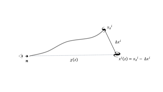
Figure 1: Positions a galaxy both on the light-cone and in real-space.

The observed galaxy overdensity is a function of the observed direction ${\bf n}$ (or, equivalenlty, $n^{i}$) and redshift $z$ (see Fig. 1) and the equivalent relation in redshift space is

$$N=\int_{{V}}{a^{3}(x^{0})\,n_{\rm g}\left(x^{0},{\bf x}\right)}\,\mathrm{d}^{3}{\bf x}\;.$$ (8)

where the observed comoving volume is $\mathrm{d}^{3}{\bf x}=\mathrm{d}V$ and $n_{\rm g}(x^{0},{\bf x})$ is the observed galaxy density. Then, by equating the total number of galaxies $N$ in Eqs. (7) and (8) and expanding to linear order in the perturbations, we can write the matter density contrast in redshift space as

$$\Delta_{\rm g}=\delta_{\rm g}+\Delta_{\rm RSD}\;,$$ (9)

where

$$\delta_{\rm g}(x^{\alpha}(z))={n_{\rm g}(x^{\alpha}(z))-\bar{n}_{\rm g}(z)\over\bar{n}_{\rm g}(z)}\;,$$

where $\bar{n}_{\rm g}(z)$ is the average density of galaxies at the observed redshift $z$. We have conveniently collected the corrections due to the metric distortions into the term $\Delta_{\rm RSD}$, e.g. see (Yoo:2008tj, ; Yoo:2009au, ; Bonvin:2011bg, ; Challinor:2011bk, ; Jeong:2011as, ). It is important to notice that $\Delta_{\rm RSD}$ receives contributions from three terms: the determinant $\sqrt{-g_{\rm R}(x_{\rm R})}$, the spatial Jacobian determinant of the mapping from real to redshift space and $[a_{\rm R}(x_{\rm R})]^{3}\,n^{\rm R}_{\rm g}(x_{\rm R})$.

In order to write explicitly the above terms we need to choose a gauge. To correctly incorporate galaxy bias in the expression for the overdensity we should treat the galaxy bias using the synchronous-comoving gauge. This gauge is entirely appropriate to describe the matter overdensity. Indeed, in this gauge, the bias is defined in the rest frame of CDM which is assumed to coincide with the rest frame of galaxies on large scales. Finally, in $\Lambda$CDM, the CDM rest frame is defined in the synchronous-comoving gauge, in which the galaxy and matter overdensities are gauge invariant, e.g. see Jeong:2011as . The synchronous-comoving gauge is defined by $g_{00}=-1$, $g_{0i}=0$ and $v^{i}=0$ (where $v^{i}$ is the galaxy peculiar velocity) and, at linear order, it turns out

$$ds^{2}=a_{\rm R}^{2}(\eta_{\rm R})\Big{\{}-\mathrm{d}\eta_{\rm R}^{2}+\Big{[}\big{(}1-2{\cal R}\big{)}\delta_{ij}+2\partial_{i}\partial_{j}E\Big{]}\mathrm{d}x_{\rm R}^{i}\mathrm{d}x_{\rm R}^{j}\Big{\}}.$$ (10)

where, in $\Lambda$CDM, we have ${\cal R}^{\prime}=0$ Ma:1995ey ; Matarrese:1997ay (a prime denotes $\partial_{\eta}$).

We can write the observed overdensity at observed redshift $z$ and in the unit direction ${\bf n}$ as

$$\Delta_{\rm g}({\bf n},z)={\Delta}_{\rm loc}({\bf n},z)+{\Delta}_{\kappa}({\bf n},z)+{\Delta}_{\rm I}({\bf n},z)+\Delta_{o}({\bf n},z)\;.$$ (11)

Here ${\Delta}_{\rm loc}$ is a local term evaluated at the source, which includes the galaxy density perturbation, the redshift distortion and the change in volume entailed by the redshift perturbation. ${\Delta}_{\kappa}$ is the weak lensing convergence integral along the line of sight, ${\Delta}_{\rm I}$ is a time delay integral along the line sight and $\Delta_{o}$ incorporates all the terms that are evaluated at the observer. In the gauge, i.e. using Eq. (10), we have Jeong:2011as

$${\Delta}_{\rm loc} = b\delta+\left[b_{e}-\left(1+2\mathcal{Q}\right)+\frac{(1+{z})}{H}\frac{dH}{dz}-\frac{2}{{\chi}}\left(1-\mathcal{Q}\right)\frac{(1+{z})}{H}\right]\left(\partial_{\|}E^{\prime}+E^{\prime\prime}\right)$$ (12)

$$-\frac{(1+{z})}{H}\partial^{2}_{\|}E^{\prime}-\frac{2}{{\chi}}\left(1-\mathcal{Q}\right)\left(\chi{\cal R}+E^{\prime}\right)\;,$$

$${\Delta}_{\kappa} = \left(1-\mathcal{Q}\right)\nabla^{2}_{\perp}\int_{0}^{{\chi}}d\tilde{\chi}\left({\chi}-\tilde{\chi}\right)\frac{{\chi}}{\tilde{\chi}}\left(E^{\prime\prime}-{\cal R}\right)\;,$$ (13)

$${\Delta}_{\rm I} = -\frac{2}{{\chi}}\left(1-\mathcal{Q}\right)\int_{0}^{{\chi}}d\tilde{\chi}\left(E^{\prime\prime}-{\cal R}\right)$$ (14)

$$+\left[b_{e}-\left(1+2\mathcal{Q}\right)+\frac{(1+{z})}{H}\frac{dH}{dz}-\frac{2}{{\chi}}\left(1-\mathcal{Q}\right)\frac{(1+{z})}{H}\right]\int_{0}^{{\chi}}d\tilde{\chi}E^{\prime\prime\prime}\;,$$

$${\Delta}_{o} = \left[3-b_{e}-\frac{(1+{z})}{H}\frac{dH}{dz}+\frac{2}{{\chi}}\left(1-\mathcal{Q}\right)\frac{(1+{z})}{H}\right](\partial_{\|}E^{\prime})_{o}$$ (16)

$$+\left[-b_{e}+\left(1+2\mathcal{Q}\right)-\frac{(1+{z})}{H}\frac{dH}{dz}+\frac{2}{{\chi}}\left(1-\mathcal{Q}\right)\frac{(1+{z})}{H}\right](E^{\prime\prime})_{o}+\frac{2}{{\chi}}\left(1-\mathcal{Q}\right)(E^{\prime})_{o}\;,$$

where $\chi(z)$ is the comoving distance, $b({z})$ is the bias,

$$\mathcal{Q}({z})={\partial\ln N_{\rm g}\over\partial\ln\mathcal{L}}\Big{|}_{\mathcal{L}=\mathcal{L}_{\rm lim}},$$ (17)

is the magnification bias Jeong:2011as and

$$b_{e}({z})=-(1+{z}){\partial\ln N_{\rm g}\over\partial z}$$ (18)

is the evolution bias. Here $N_{\rm g}=a^{3}n_{\rm g}$ denotes the comoving number density of galaxies with luminosity larger than $L$ and the derivative is evaluated at the (redshift-dependent) limiting luminosity of the survey. Finally, the directional derivatives are defined as

$$\partial_{\|}=n^{j}\partial_{j},~{}~{}~{}\partial_{\|}^{i}=n^{i}\partial_{\|}\;,~{}~{}~{}\partial_{\|}^{2}=\partial_{\|i}\partial_{\|}^{i}=\partial_{\|}\partial_{\|},~{}~{}\partial_{\perp}^{i}=(\delta^{ij}-n^{i}n^{j})\partial_{j}\;,~{}~{}~{}\nabla^{2}_{\perp}=\partial_{\perp i}\partial_{\perp}^{i}=\nabla^{2}-\partial_{\|}^{2}-2{\chi}^{-1}\partial_{\|}.$$ (19)

The local term $\Delta_{\rm loc}$ contains the Newtonian local terms, and in addition some GR corrections. The line of sight term $\Delta_{\rm I}$ is a pure GR correction. The lensing term $\Delta_{\kappa}$ is the same as in the Newtonian analysis. It is useful to relate the metric perturbations to the matter density contrast in synchronous gauge. Removing the residual gauge ambiguity and consequently and using

$$E^{\prime\prime}+aHE^{\prime}-4\pi G\rho_{m}E=0\,,$$ (20)

we obtain

$$E^{\prime} = -\frac{H}{(1+z)}f\nabla^{-2}\delta,$$ (21)

$$E^{\prime\prime} = -\frac{H^{2}}{(1+z)^{2}}\Big{(}\frac{3}{2}\Omega_{\rm m}-f\Big{)}\nabla^{-2}\delta,$$ (22)

$$E^{\prime\prime\prime} = -3\frac{H^{3}}{(1+z)^{3}}\Omega_{\rm m}\left(f-1\right)\nabla^{-2}\delta,$$ (23)

$${\cal R} = \frac{H^{2}}{(1+z)^{2}}\Big{(}\frac{3}{2}\Omega_{\rm m}+f\Big{)}\nabla^{-2}\delta.$$ (24)

Here $\Omega_{\rm m}(z)$ is the matter density and $f(z)$ is the growth rate,

$$f={d\ln D\over d\ln a},~{}~{}~{}\delta({\bf x},z)=\delta({\bf x},0){D(z)\over D(0)},$$ (25)

where $D$ is the growing mode of $\delta$. For intensity mapping surveys of the HI 21cm emission (e.g. Abdalla:2004ah ), Hall:2012wd ; Alonso:2015uua pointed out that we can use the above ration assuming $\mathcal{Q}=1$ and hence $\Delta_{\kappa}=0$. In other words,

$$\Delta_{\rm IM}({\bf n},z)=\Delta_{\rm g}({\bf n},z,\mathcal{Q}=1)\;.$$ (26)

III Dipole

Via Scaccabarozzi:2018vux we know that the most important contribution in ${\Delta}_{o}$ is the dipole and all the other terms are negligible (at least for $z<5-10$) for scales less than $1/H_{0}$. [For a further discussion about this point see the comment below Eq. (IV).] In other words, we are able to simplify this quantity as

$${\Delta}_{o}\simeq{\Delta}_{v_{\|}o}=\left[3-b_{e}-\frac{(1+{z})}{H}\frac{dH}{dz}+\frac{2}{{\chi}}\left(1-\mathcal{Q}\right)\frac{(1+{z})}{H}\right](\partial_{\|}E^{\prime})_{o}\;.$$ (27)

Then from now on we will consider only the following quantity

$$\Delta_{\rm g}=\Delta+{\Delta}_{v_{\|}o}\quad{\rm where}\quad\Delta={\Delta}_{\rm loc}+{\Delta}_{\kappa}+{\Delta}_{\rm I}$$ (28)

In this case we have to generalise the results computed in Bertacca:2012tp and we need to understand if this local effect is really relevant and/or the same order of GR and wide-angle contributions. Here below we shortly review the results obtained in Refs.  Bertacca:2012tp ; Raccanelli:2013multipoli (see also Raccanelli:2013gja where they analyzed in details the integrated effects), and in the section V we study the dipole effect within the two point correlation function.

IV Redshift-space correlation function using only $\Delta$.

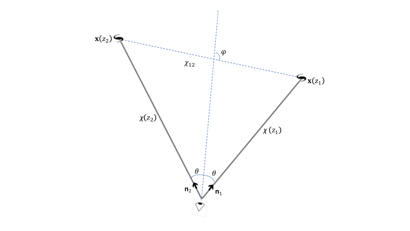
Figure 2: Geometry of the problem: the triangle formed by the observer and the pair of galaxies on the lightcone.

First of all, let us start to compute the observed galaxy correlation function (see Fig. 2):

$$\xi_{\Delta}({\bf x}_{1},{\bf x}_{2})=\xi_{\Delta}({\bf n}_{1},{\bf n}_{2},z_{1},z_{2})=\langle\Delta({\bf n}_{1},z_{1})\Delta({\bf n}_{2},z_{2})\rangle\,.$$ (29)

where ${\bf x}$ is related to the comoving distance $\chi$ by

$${\bf x}=\chi(z){\bf n},~{}~{}\chi(z)=\int_{0}^{z}{dz^{\prime}\over H(z^{\prime})}.$$ (30)

In Bertacca:2012tp the authors applied the decomposition used in previous analyses based on Szalay:1997cc ; Bharadwaj:1998bq ; Matsubara:1999du ; Szapudi:2004gh ; Papai:2008bd where they expanded the redshift space correlation function using tripolar spherical harmonics, with the basis following functions

$$S_{\ell_{1}\ell_{2}L}({{{\bf n}}}_{1},{{{\bf n}}}_{2},{{{\bf n}}}_{12})=\left[{(4\pi)^{3}\over(2\ell_{1}+1)(2\ell_{2}+1)(2L+1)}\right]^{1/2}\!\sum_{m_{1},m_{2},M}\left(\begin{array}[]{ccc}\ell_{1}&\ell_{2}&L\\ m_{1}&m_{2}&M\end{array}\right)Y_{\ell_{1}m_{1}}({{{\bf n}}}_{1})Y_{\ell_{2}m_{2}}({{{\bf n}}}_{2})Y_{LM}({{{\bf n}}}_{12}),$$ (33)

where

$$-\ell_{1}\leq m_{1}\leq\ell_{1}\;,\quad-\ell_{2}\leq m_{2}\leq\ell_{2}\;,\quad-L\leq M\leq L,\quad{\rm and}\quad\left(\begin{array}[]{ccc}\ell_{1}&\ell_{2}&\ell_{3}\\ m_{1}&m_{2}&m_{3}\end{array}\right)$$

is the Wigner 3$j$ symbol (see also Raccanelli:2010hk ; Samushia:2011cs ; Raccanelli:2013multipoli ; Raccanelli:2013gja ; Raccanelli:2016avd ). Then the correlation functions in redshift space can be written in the following way:

$$\xi_{AB}({\bf x}_{1},{\bf x}_{2})=\langle\Delta_{A}({\bf x}_{1})\Delta_{B}({\bf x}_{2})\rangle=\xi_{BA}({\bf x}_{2},{\bf x}_{1}),\quad{\rm where}\quad A,B={\rm loc,\kappa,I}\,.$$ (35)

First of all, let us define the tensor $\mathcal{A}$ which spherical transforms the matter overdensity as Szalay:1997cc

$$\mathcal{A}^{n}_{\ell}({\bf x},z)=\int\frac{d^{3}k}{(2\pi)^{3}}\,{\mathcal{P}_{\ell}({{\bf n}}\cdot{\hat{\bf k}})\over(ik)^{n}}~{}{\rm e}^{i{\bf k}\cdot{\bf x}}\;\delta({\bf k},z)\,,$$ (36)

where ${\bf x}=\chi{\bf n}$, $\mathcal{P}_{\ell}$ is a Legendre polynomial. For simplicity, we start with considering only local terms. Using the decomposition relation by Eq. (36), Eq. (12) turns out

$$\Delta_{\rm loc}=b\left[\left(1+\frac{1}{3}\beta\right)\mathcal{A}^{0}_{0}+\gamma\mathcal{A}^{2}_{0}+\frac{\beta\alpha}{\chi}\mathcal{A}^{1}_{1}+\frac{2}{3}\beta\mathcal{A}^{0}_{2},\right]$$ (37)

where

$$\alpha(z) = \alpha_{\rm Nwt}(z)-\frac{\chi(z)H(z)}{(1+z)}\left[\frac{3}{2}\Omega_{\rm m}(z)-1-2\mathcal{Q}(z)\right]\;,$$ (38)

$$\beta(z) = \frac{f(z)}{b(z)},~{}~{}~{}~{}f=-{d\ln D(z)\over d\ln(1+z)}\;,$$ (39)

$$\gamma(z) = \frac{H(z)}{(1+z)}\left\{\frac{H(z)}{(1+z)}\left[\beta(z)-\frac{3}{2}\frac{\Omega_{\rm m}(z)}{b(z)}\right]b_{e}(z)+\frac{3}{2}\frac{H(z)}{(1+z)}\beta(z)\big{[}\Omega_{\rm m}(z)-2\big{]}\right.$$ (40)

$$\left.-\frac{3}{2}\frac{H(z)}{(1+z)}\frac{\Omega_{\rm m}(z)}{b(z)}\left[1-4\mathcal{Q}(z)+\frac{3}{2}\Omega_{\rm m}(z)\right]+\frac{3}{\chi(z)}\big{[}1-\mathcal{Q}(z)\big{]}\frac{\Omega_{\rm m}(z)}{b(z)}\right\}\,.$$

Here

$${\alpha_{\rm Nwt}(z)\over\chi(z)}=-\frac{H(z)}{(1+z)}\left\{b_{e}(z)-\frac{2}{\chi(z)}\big{[}1-\mathcal{Q}(z)\big{]}\frac{(1+z)}{H(z)}\right\}=\frac{d\ln{N_{\rm g}}}{d\chi}+\big{[}1-\mathcal{Q}(z)\big{]}\frac{2}{\chi}\;.$$ (41)

is the Newtonian usual part of $\alpha$ considered in Hamilton:1997zq . Note that considering a $\Lambda$CDM background, we have used in the above relations the following identity $(1+z)/H\,(\partial H/\partial z)=3\Omega_{\rm m}(z)/2$. Correlating the tensor $\mathcal{A}$ [defined in Eq. (36) ], we have

$${\mathcal{S}}_{\ell_{1}\ell_{2}}^{n_{1}+n_{2}}(z_{1},z_{2};{\bf n}_{1},{\bf n}_{2}) \equiv \langle\mathcal{A}^{n_{1}}_{\ell_{1}}({\bf x}_{1},{z}_{1})\mathcal{A}^{n_{2}}_{\ell_{2}}({\bf x}_{2},{z}_{2})\rangle$$ (42)

$$= (-1)^{\ell_{2}}\int\frac{d^{3}k}{(2\pi)^{3}}(ik)^{-(n_{1}+n_{2})}\mathcal{P}_{\ell_{1}}({\hat{\bf k}}\cdot{\bf n}_{1})\mathcal{P}_{\ell_{2}}({\hat{\bf k}}\cdot{\bf n}_{2})\exp{\left(i{\bf k}\cdot{\bf x}_{12}\right)}\;P_{\delta}(k;{z}_{1},{z}_{2})\;,$$

where ${\bf x}_{12}={\bf x}_{1}-{\bf x}_{2}\equiv\chi_{12}{\bf n}_{12}$ and $P_{\delta}(k;{z}_{1},{z}_{2})$ it the power spectrum. Here we have used the identity $\mathcal{P}_{\ell}(-{\hat{\bf k}}\cdot{\bf n})=(-1)^{\ell}\mathcal{P}_{\ell}({\hat{\bf k}}\cdot{\bf n})$. Expanding in spherical harmonics

$$\mathcal{P}_{\ell}({{\bf n}}\cdot\hat{\bf k})=\frac{4\pi}{2\ell+1}\sum_{m=-\ell}^{\ell}Y^{*}_{\ell m}(\hat{\bf k})Y_{\ell m}({\bf n})$$ (43)

and

$${\rm e}^{i{\bf k}\cdot{\bf x}}=4\pi\sum_{\ell=0}^{\infty}\sum_{m=-\ell}^{\ell}i^{\ell}j_{\ell}(\chi k)Y^{*}_{\ell m}(\hat{\bf k})Y_{\ell m}({\bf n})\,,$$ (44)

and applying the Gaunt integral

$$\int{\rm d}^{2}\hat{\bf k}~{}Y_{\ell_{1}m_{1}}(\hat{\bf k})Y_{\ell_{2}m_{2}}(\hat{\bf k})Y_{\ell_{3}m_{3}}(\hat{\bf k}) = \sqrt{\frac{(2\ell_{1}+1)(2\ell_{2}+1)(2\ell_{3}+1)}{4\pi}}\left(\begin{array}[]{ccc}\ell_{1}&\ell_{2}&\ell_{3}\\ 0&0&0\end{array}\right)\left(\begin{array}[]{ccc}\ell_{1}&\ell_{2}&\ell_{3}\\ m_{1}&m_{2}&m_{3}\end{array}\right)\;,$$ (49)

we find

$${\mathcal{S}}_{\ell_{1}\ell_{2}}^{n_{1}+n_{2}}(z_{1},z_{2};{\bf n}_{1},{\bf n}_{2}) = \sum_{L}(-1)^{\ell_{2}}\;i^{L-n_{1}-n_{2}}\left(\begin{array}[]{ccc}\ell_{1}&\ell_{2}&L\\ 0&0&0\end{array}\right)S_{\ell_{1}\ell_{2}L}({\bf n}_{1},{\bf n}_{2},{\bf n}_{12})\,\xi_{L}^{n_{1}+n_{2}}(\chi_{12};z_{1},z_{2}),$$

$$|\ell_{1}-\ell_{2}|\leq L\leq\ell_{1}+\ell_{2},$$

where we used the tripolar basis defined in (33). Here, we have defined

$$\xi_{L}^{n}(\chi;z_{1},z_{2})=\int\frac{dk}{2\pi^{2}}k^{2-n}j_{L}(\chi k)\,P_{\delta}(k;z_{1},z_{2})$$ (54)

which describes the spherical Bessel transformation of the matter power spectrum $P_{\delta}(k;z_{1},z_{2})$ Szalay:1997cc . Finally, using the tripolar decomposition of $\xi_{loc}$, we find

$${\xi}_{\rm loc}({\bf x}_{1},z_{1},{\bf x}_{2},z_{2})=b(z_{1})b(z_{2})\sum_{\ell_{1},\ell_{2},L,n}{\left(B_{\rm loc\,loc}\right)}_{n}^{\,\ell_{1}\ell_{2}L}({\chi}_{1},{\chi}_{2})\,S_{\ell_{1}\ell_{2}L}({{{\bf n}}}_{1},{{{\bf n}}}_{2},{{{\bf n}}}_{12})\,\xi_{L}^{\,n}(\chi_{12};z_{1},z_{2})\,.$$ (55)

The ${\left(B_{\rm loc\,loc}\right)}_{n}^{\,\ell_{1}\ell_{2}L}$ coefficients contain the local corrections due to the functions $\alpha$, $\beta$ and $\gamma$ Bertacca:2012tp .

Furthermore another very interesting expression of the local correlation function can be achieved if we rewrite the tripolar spherical harmonics basis $S_{\ell_{1}\ell_{2}L}$ as the combination of two Legendre polynomials which depend on the angular dependence $\varphi$ and $\theta$, see Fig. 2. This method appears to be more natural for looking at the behaviour of the multipoles. Then we can obtain the following decomposition

$$\xi_{\rm loc}(z_{2},\theta,\varphi)=b(z_{1})b(z_{2})\sum_{\tilde{L},\tilde{\ell}}\;C_{\tilde{L}\tilde{\ell}_{3}}(z_{2},\theta,\varphi)\;\mathcal{P}_{\tilde{L}}(\cos\varphi)\;\mathcal{P}_{\tilde{\ell_{3}}}(\cos\theta)$$ (56)

and the coefficients $C_{\tilde{L}\tilde{\ell}_{3}}$ are given Raccanelli:2013multipoli

$$C_{00} = \left(1+\frac{\beta_{1}}{3}+\frac{\beta_{2}}{3}+\frac{29}{225}\beta_{1}\beta_{2}\right)\xi_{0}^{0}-\left(\gamma_{1}+\gamma_{2}+\frac{1}{3}\beta_{1}\gamma_{2}+\frac{1}{3}\gamma_{1}\beta_{2}+\frac{1}{9}\beta_{1}\beta_{2}\frac{\alpha_{1}}{\chi_{1}}\frac{\alpha_{2}}{\chi_{2}}\right)\xi^{2}_{0}+$$

$$+\gamma_{1}\gamma_{2}\xi^{4}_{0}+\sin\varphi\sin\theta\left[\left(1+\frac{1}{3}\beta_{1}\right)\beta_{2}\frac{\alpha_{2}}{\chi_{2}}+\left(1+\frac{1}{3}\beta_{2}\right)\beta_{1}\frac{\alpha_{1}}{\chi_{1}}\right]\xi_{1}^{1}+$$

$$-\sin\varphi\sin\theta\left(\gamma_{1}\beta_{2}\frac{\alpha_{2}}{\chi_{2}}+\beta_{1}\frac{\alpha_{1}}{\chi_{1}}\gamma_{2}\right)\xi^{3}_{1}-\left(\frac{2}{9}\beta_{1}+\frac{2}{9}\beta_{2}+\frac{44}{315}\beta_{1}\beta_{2}\right)\xi^{0}_{2}+$$

$$+\frac{2}{9}\left(\beta_{1}\beta_{2}\frac{\alpha_{1}}{\chi_{1}}\frac{\alpha_{2}}{\chi_{2}}+\gamma_{1}\beta_{2}+\beta_{1}\gamma_{2}\right)\xi^{2}_{2}+\frac{32}{1575}\beta_{1}\beta_{2}\xi^{0}_{4}\;,$$

$$C_{11} = \left[-\left(1+\frac{7}{25}\beta_{1}\right)\beta_{2}\frac{\alpha_{2}}{\chi_{2}}+\left(1+\frac{7}{25}\beta_{2}\right)\beta_{1}\frac{\alpha_{1}}{\chi_{1}}\right]\xi_{1}^{1}+\left(\gamma_{1}\beta_{2}\frac{\alpha_{2}}{\chi_{2}}-\beta_{1}\frac{\alpha_{1}}{\chi_{1}}\gamma_{2}\right)\xi^{3}_{1}+$$

$$+2\sin\varphi\sin\theta\left(\beta_{2}-\beta_{1}\right)\xi^{0}_{2}+2\sin\varphi\sin\theta\left(\beta_{1}\gamma_{2}-\gamma_{1}\beta_{2}\right)\xi^{2}_{2}+\frac{2}{25}\left(\beta_{1}\frac{\alpha_{1}}{\chi_{1}}\beta_{2}-\beta_{1}\beta_{2}\frac{\alpha_{2}}{\chi_{2}}\right)\xi^{1}_{3}\;,$$

$$C_{02} = -\frac{16}{315}\beta_{1}\beta_{2}\xi_{0}^{0}+\frac{4}{9}\beta_{1}\beta_{2}\frac{\alpha_{1}}{\chi_{1}}\frac{\alpha_{2}}{\chi_{2}}\xi^{2}_{0}-\frac{8}{15}\sin\varphi\sin\theta\beta_{1}\beta_{2}\left(\frac{\alpha_{1}}{\chi_{1}}+\frac{\alpha_{2}}{\chi_{2}}\right)\xi_{1}^{1}+$$

$$+\left(\frac{2}{9}\beta_{1}+\frac{2}{9}\beta_{2}+\frac{100}{441}\beta_{1}\beta_{2}\right)\xi^{0}_{2}-\frac{2}{9}\left(\beta_{1}\beta_{2}\frac{\alpha_{1}}{\chi_{1}}\frac{\alpha_{2}}{\chi_{2}}+\gamma_{1}\beta_{2}+\beta_{1}\gamma_{2}\right)\xi^{2}_{2}\;+$$

$$+\frac{2}{15}\sin\varphi\sin\theta\beta_{1}\beta_{2}\left(\frac{\alpha_{1}}{\chi_{1}}+\frac{\alpha_{2}}{\chi_{2}}\right)\xi_{3}^{1}-\frac{88}{2205}\beta_{1}\beta_{2}\xi^{0}_{4}\;,$$

$$C_{20} = \left(\frac{2}{9}\beta_{1}+\frac{2}{9}\beta_{2}+\frac{4}{21}\beta_{1}\beta_{2}\right)\xi^{0}_{2}-\frac{2}{9}\left(3\beta_{1}\beta_{2}\frac{\alpha_{1}}{\chi_{1}}\frac{\alpha_{2}}{\chi_{2}}+\gamma_{1}\beta_{2}+\beta_{1}\gamma_{2}\right)\xi^{2}_{2}\;+$$

$$+\frac{2}{3}\sin\varphi\sin\theta\beta_{1}\beta_{2}\left(\frac{\alpha_{1}}{\chi_{1}}+\frac{\alpha_{2}}{\chi_{2}}\right)\xi_{3}^{1}-\frac{8}{63}\beta_{1}\beta_{2}\xi^{0}_{4}\;,$$

$$C_{22} = -\left(\frac{8}{9}\beta_{1}+\frac{8}{9}\beta_{2}+\frac{16}{21}\beta_{1}\beta_{2}\right)\xi^{0}_{2}+\frac{8}{9}\left(\gamma_{1}\beta_{2}+\beta_{1}\gamma_{2}\right)\xi^{2}_{2}\;+\frac{8}{63}\beta_{1}\beta_{2}\xi^{0}_{4}\;,$$

$$C_{13} = \frac{8}{25}\beta_{1}\beta_{2}\left(\frac{\alpha_{1}}{\chi_{1}}-\frac{\alpha_{2}}{\chi_{2}}\right)\xi^{1}_{1}-\frac{2}{25}\beta_{1}\beta_{2}\left(\frac{\alpha_{1}}{\chi_{1}}-\frac{\alpha_{2}}{\chi_{2}}\right)\xi^{1}_{3}\;,$$

$$C_{31} = -\frac{2}{5}\beta_{1}\beta_{2}\left(\frac{\alpha_{1}}{\chi_{1}}-\frac{\alpha_{2}}{\chi_{2}}\right)\xi^{1}_{3}\;,$$

$$C_{04} = \frac{64}{525}\beta_{1}\beta_{2}\xi^{0}_{0}-\frac{64}{735}\beta_{1}\beta_{2}\xi^{0}_{2}+\frac{24}{1225}\beta_{1}\beta_{2}\xi^{0}_{4}\;,$$

$$C_{40} = \frac{8}{35}\beta_{1}\beta_{2}\xi^{0}_{4}\;,$$ (57)

where a subscript $i$ denotes evaluation at $z_{i}$.

At this stage, it is important to make the following comment; as it was pointed out in Bertacca:2012tp for $n=4$ and $L=0$, $\xi_{L}^{n}$ is divergence and as correctly observed in Scaccabarozzi:2018vux , it is not a real divergence. However, this issue comes form the fact that we have neglected terms evaluated at the observer position, i.e. $\Delta_{o}$, in the above calculation. Instead, if we consider all terms in Eq.(11), the sum of all individually divergent contributions in the correlation function is instead finite in agreement with the equivalence principle Scaccabarozzi:2018vux . The above prescription is still correct if we safely impose an IR cut-off scale, as long as $k_{\rm min}\lesssim H_{0}$ and $k_{\rm min}\leq k$ when we compute the integrals in Eq. (54). (Let us point out that in Bertacca:2012tp they took as $k_{\rm min}\sim H_{0}/2$.) Contrarily, as will we see later, the dipole which is a non divergent contribution in $\Delta_{o}$ will play an important role within correlation function. Precisely, as we see in Section V, the dipole correction will add several new terms and effects on the galaxy two point correlation function.

IV.1 Non-local terms

The remaining $\xi_{AB}$ all involve integrals along the lines of sight. The spherical transforms of $\Delta_{\kappa},\Delta_{I}$ are (for further details, see Bertacca:2012tp )

$$\Delta_{\kappa}({\bf n},z) = b(z)\int^{\chi}{d\tilde{\chi}}\;\sigma(z,\tilde{z})\left[\mathcal{A}^{0}_{0}(\tilde{\bf x},\tilde{z})-\mathcal{A}^{0}_{2}(\tilde{\bf x},\tilde{z})-\frac{3}{\tilde{\chi}}\mathcal{A}^{1}_{1}(\tilde{\bf x},\tilde{z})\right],$$ (61)

$$\Delta_{\rm I}({\bf n},z) = b(z)\int^{\chi}{d\tilde{\chi}}\;\mu(z,\tilde{z})\mathcal{A}^{2}_{0}(\tilde{\bf x},\tilde{z}),$$ (62)

where

$$\sigma(z,\tilde{z}) \equiv -2\frac{H^{2}(\tilde{z})}{(1+\tilde{z})^{2}}\frac{\left({\chi}-\tilde{\chi}\right)\tilde{\chi}}{{\chi}}\frac{\big{[}1-\mathcal{Q}(z)\big{]}}{b({z})}\Omega_{\rm m}(\tilde{z}),$$ (63)

$$\mu(z,\tilde{z}) \equiv 3\frac{H^{2}(\tilde{z})}{(1+\tilde{z})^{2}}\frac{\Omega_{\rm m}(\tilde{z})}{b({z})}\Bigg{\{}\frac{2}{{\chi}}\big{[}1-\mathcal{Q}(z)\big{]}-\frac{H(\tilde{z})}{(1+\tilde{z})}\big{[}f(\tilde{z})-1\big{]}\bigg{[}b_{e}({z})-\big{[}1+2\mathcal{Q}(z)\big{]}+\frac{3}{2}\Omega_{\rm m}({z})$$

$$-\frac{2}{{\chi}}\big{[}1-\mathcal{Q}(z)\big{]}\frac{(1+{z})}{H({z})}\bigg{]}\Bigg{\}},$$

and $\chi=\chi(z),\tilde{\chi}=\chi(\tilde{z})$. Let us point out that in Eq. (61) we used the definition (19). Then the lensing-lensing correlation turns out

$${\xi}_{\kappa\kappa}({\bf x}_{1},{\bf x}_{2})=b(z_{1})b(z_{2})\int^{{\chi}_{1},\chi_{2}}{d\tilde{\chi}_{1}}{d\tilde{\chi}_{2}}\sum_{\ell_{1},\ell_{2},L,n}\left(B_{\kappa\kappa}\right)_{n}^{\ell_{1}\ell_{2}L}({\chi}_{1},\tilde{\chi}_{1};{\chi}_{2},\tilde{\chi}_{2})\,S_{\ell_{1}\ell_{2}L}({{{\bf n}}}_{1},{{{\bf n}}}_{2},{\tilde{\bf n}}_{12})\,\xi_{L}^{n}(\tilde{\chi}_{12};\tilde{z}_{1},\tilde{z}_{2}),$$ (65)

and for the ${\rm II}$ correlation we find

$${\xi}_{\rm II}({\bf x}_{1},{\bf x}_{2})=b(z_{1})b(z_{2})\int^{{\chi}_{1},\chi_{2}}{d\tilde{\chi}_{1}}{d\tilde{\chi}_{2}}\sum_{\ell_{1},\ell_{2},L,n}\left(B_{\rm II}\right)_{n}^{\ell_{1}\ell_{2}L}({\chi}_{1},\tilde{\chi}_{1};{\chi}_{2},\tilde{\chi}_{2})\,S_{\ell_{1}\ell_{2}L}({{{\bf n}}}_{1},{{{\bf n}}}_{2},{\tilde{\bf n}}_{12})\,\xi_{L}^{n}(\tilde{\chi}_{12};\tilde{z}_{1},\tilde{z}_{2}).$$ (66)

The integration variables ${\tilde{\chi}_{12}},{\tilde{\bf n}}_{12}$ are given by

$${\tilde{\chi}_{12}}{\tilde{\bf n}}_{12}={\chi}_{12}{{{\bf n}}}_{12}+\left(\tilde{\chi}_{1}-{\chi}_{1}\right){{{\bf n}}}_{1}-\left(\tilde{\chi}_{2}-{\chi}_{2}\right){{{\bf n}}}_{2},\quad\quad{\rm and}\quad\quad\tilde{\chi}^{2}_{12}={\tilde{\chi}_{1}^{2}+\tilde{\chi}_{2}^{2}+\frac{\tilde{\chi}_{1}\tilde{\chi}_{2}}{{\chi}_{1}{\chi}_{2}}\left[{\chi}_{12}^{2}-\left({\tilde{\chi}}_{1}^{2}+{\tilde{\chi}}_{2}^{2}\right)\right]}.$$ (67)

Similarly, we find:

$${\xi}_{\rm loc\,I}({\bf x}_{1},{\bf x}_{2})=b(z_{1})b(z_{2})\int^{{\chi}_{2}}{d\tilde{\chi}_{2}}\sum_{\ell_{1},\ell_{2},L,n}\left(B_{\rm loc\,I}\right)_{n}^{\ell_{1}\ell_{2}L}({\chi}_{1};{\chi}_{2},\tilde{\chi}_{2})S_{\ell_{1}\ell_{2}L}({{{\bf n}}}_{1},{{{\bf n}}}_{2},{{\bf n}}_{1\tilde{2}})\,\xi_{L}^{n}(\chi_{1\tilde{2}};{z}_{1},\tilde{z}_{2})\;,$$ (68)

$${\xi}_{\rm loc\,\kappa}({\bf x}_{1},{\bf x}_{2})=b(z_{1})b(z_{2})\int^{{\chi}_{2}}{d\tilde{\chi}_{2}}\sum_{\ell_{1},\ell_{2},L,n}\left(B_{\rm loc\,\kappa}\right)_{n}^{\ell_{1}\ell_{2}L}({\chi}_{1};{\chi}_{2},\tilde{\chi}_{2})S_{\ell_{1}\ell_{2}L}({{{\bf n}}}_{1},{{{\bf n}}}_{2},{{\bf n}}_{1\tilde{2}})\,\xi_{L}^{n}(\chi_{1\tilde{2}};{z}_{1},\tilde{z}_{2})\;,$$ (69)

$${\xi}_{\rm\kappa\,I}({\bf x}_{1},{\bf x}_{2})=b(z_{1})b(z_{2})\int^{{\chi}_{1},\chi_{2}}{d\tilde{\chi}_{1}}{d\tilde{\chi}_{2}}\sum_{\ell_{1},\ell_{2},L,n}\left(B_{\rm\kappa\,I}\right)_{n}^{\ell_{1}\ell_{2}L}({\chi}_{1},\tilde{\chi}_{1};{\chi}_{2},\tilde{\chi}_{2})\,S_{\ell_{1}\ell_{2}L}({{{\bf n}}}_{1},{{{\bf n}}}_{2},{\tilde{\bf n}}_{12})\,\xi_{L}^{n}(\tilde{\chi}_{12};\tilde{z}_{1},\tilde{z}_{2})\;,$$

(70)

where

$$\chi_{1\tilde{2}}{{\bf n}}_{{1}\tilde{2}}={\left({\chi}_{2}-\tilde{\chi}_{2}\right){{{\bf n}}}_{2}+{\chi}_{12}{{{\bf n}}}_{12}}\;,\quad\quad{\rm and}\quad\quad\chi_{1\tilde{2}}^{2}={{\chi}_{1}^{2}+\tilde{\chi}_{2}^{2}+\frac{\tilde{\chi}_{2}}{{\chi}_{2}}\left[{\chi}_{12}^{2}-\left({\chi}_{1}^{2}+{\chi}_{2}^{2}\right)\right]}.$$ (71)

We can obtain the remaining $\xi_{AB}$ by using the symmetry in (35). In Ref. Bertacca:2012tp , the authors have explicitly computed the above coefficients $B_{AB\;n}^{\phantom{AB\;}\ell_{1}\ell_{2}L}({\chi}_{1},\tilde{\chi}_{1};{\chi}_{2},\tilde{\chi}_{2})$, where $A,B={\rm loc},\,\kappa,\,{\rm I}$. (As we have already pointed out above, we have replaced the subscript $\rm s$ used in Bertacca:2012tp with $\rm loc$.)

V Analysis of dipole term

In this section we discuss the main part of this work, where we will discuss the effect of the local group through the dipole at the observer on two point correlation function. From Eq. (21) we know

$$E_{o}^{\prime}=(E^{\prime})_{o}({\bf n})=-H_{0}f_{0}\left[\nabla^{-2}\delta({\bf x},0)\right]_{{\bf x}\to{\bf 0}}\;,$$ (72)

where we note that ${\bf x}\to{\bf 0}$ is equivalently to $\chi\to 0$. Then

$$(\partial_{\|}E^{\prime})_{o} = -H_{0}f_{0}\left[n^{i}\partial_{i}\nabla^{-2}\delta({\bf x},0)\right]_{{\bf x}\to{\bf 0}}=-H_{0}f_{0}\left[\int\frac{d^{3}k}{(2\pi)^{3}}\frac{\mathcal{P}_{1}({\hat{\bf k}}\cdot{\bf n})}{ik}\;\delta({\bf k},0)~{}{\rm e}^{i{\bf k}\cdot{\bf x}}\right]_{{\bf x}\to{\bf 0}}$$ (73)

$$= -H_{0}f_{0}\int\frac{d^{3}k}{(2\pi)^{3}}\frac{\mathcal{P}_{1}({\hat{\bf k}}\cdot{\bf n})}{ik}\delta({\bf k},0)=-H_{0}f_{0}\left[{\mathcal{A}}_{1}^{1}({\bf x},0)\right]_{{\bf x}\to{\bf 0}}$$

and Eq. (27) turns out

$${\Delta}_{v_{\|}o}=b(z)\omega_{o}(z)\left[{\mathcal{A}}_{1}^{1}({\bf x},0)\right]_{{\bf x}\to{\bf 0}}\;.$$ (74)

In GR, the rocket effect contains new terms that depends also on the magnification bias and the expansion rate:

$${\Delta}_{v_{\|}o}=b(z)\omega_{o}(z)\int\frac{d^{3}k}{(2\pi)^{3}}\frac{\mathcal{P}_{1}({\hat{\bf k}}\cdot{\bf n})}{ik}\delta({\bf k},0)$$ (75)

where

$$\omega_{o}(z)=-{H_{0}f_{0}\over b(z)}\left[3-b_{e}(z)-{3\over 2}\Omega_{\rm m}(z)+\frac{2(1+{z})}{\chi(z)H(z)}\left(1-\mathcal{Q}(z)\right)\right]\;.$$ (76)

At this point if we want to correlate $\Delta$ with $\Delta_{o}$, we should compute the tensor $\mathcal{S}_{\ell 1\ell_{2}}^{n_{1}n_{2}}({\bf x}_{1},{\bf x}_{2})$ in three different regimes:

$${\rm 1)}\;{\mathcal{S}}_{\ell 1\ell_{2}}^{n_{1}n_{2}}({\bf x}_{1},{\bf x}_{2})\Big{|}_{\small\begin{array}[]{c}\chi_{1}\to 0\\ \chi_{2}\to 0\end{array}}\;,\quad\quad{\rm 2)}\;{\mathcal{S}}_{\ell 1\ell_{2}}^{n_{1}n_{2}}({\bf x}_{1},{\bf x}_{2})\Big{|}_{\chi_{2}\to 0}\;,\quad\quad{\rm 3)}\;{\mathcal{S}}_{\ell 1\ell_{2}}^{n_{1}n_{2}}({\bf x}_{1},{\bf x}_{2})\Big{|}_{\chi_{1}\to 0}\;.$$ (79)

V.1 ${\mathcal{S}}_{\ell 1\ell_{2}}^{n_{1}n_{2}}({\bf x}_{1},{\bf x}_{2})$ for $\chi_{1}\to 0$ and $\chi_{2}\to 0$

Using Eq. (42) we have

$${\mathcal{S}}_{\ell_{1}\ell_{2}}^{n_{1}+n_{2}}(0,0;{\bf n}_{1},{\bf n}_{2})=(-1)^{\ell_{2}}\int\frac{d^{3}k}{(2\pi)^{3}}(ik)^{-(n_{1}+n_{2})}\mathcal{P}_{\ell_{1}}({\hat{\bf k}}\cdot{\bf n}_{1})\mathcal{P}_{\ell_{2}}({\hat{\bf k}}\cdot{\bf n}_{2})\;P_{\delta}(k;{z}_{1},{z}_{2})$$

$$=(-1)^{\ell_{2}}\frac{(4\pi)^{2}}{(2\ell_{1}+1)(2\ell_{2}+1)}\sum_{m_{1}\,m_{2}}\left\{Y_{\ell_{1}m_{1}}({\bf n}_{1})Y_{\ell_{2}m_{2}}({\bf n}_{2})\left[\int\frac{d^{3}k}{(2\pi)^{3}}(ik)^{-(n_{1}+n_{2})}Y^{*}_{\ell_{1}m_{1}}(\hat{\bf k})\;Y^{*}_{\ell_{2}m_{2}}(\hat{\bf k})\;P_{\delta}(k;{z}_{1},{z}_{2})\right]\right\}$$

$$=(-1)^{\ell_{1}}\frac{(4\pi)^{2}}{(2\ell_{1}+1)^{2}}\delta^{K}_{\ell_{1}\ell_{2}}\left[\sum_{m_{1}}(-1)^{m_{1}}Y_{\ell_{1}m_{1}}({\bf n}_{1})Y_{\ell_{1}-m_{1}}({\bf n}_{2})\right]\left[\int\frac{k^{2}dk}{(2\pi)^{3}}(ik)^{-(n_{1}+n_{2})}\;P_{\delta}(k;0,0)\right]$$

$$=\frac{(-1)^{\ell_{1}}i^{-(n_{1}+n_{2})}}{(2\ell_{1}+1)^{2}}\delta^{K}_{\ell_{1}\ell_{2}}\left[\sum_{m_{1}\,m_{2}}Y_{\ell_{1}m_{1}}({\bf n}_{1})Y^{*}_{\ell_{1}m_{1}}({\bf n}_{2})\right]\left[\frac{2}{\pi}\int k^{2-(n_{1}+n_{2})}dk\;P_{\delta}(k;0,0)\right]$$

$$=\frac{(-1)^{\ell_{1}}i^{-(n_{1}+n_{2})}}{(2\ell_{1}+1)}\delta^{K}_{\ell_{1}\ell_{2}}{\mathcal{P}}_{\ell_{1}}({\bf n}_{1}\cdot{\bf n}_{2})\left[\frac{1}{2\pi^{2}}\int k^{2-(n_{1}+n_{2})}dk\;P_{\delta}(k;0,0)\right]$$ (80)

where in the second and the last line we used Eq. (43), in the third and forth line $Y^{*}_{\ell m}({\bf n})=(-1)^{m}Y_{\ell-m}({\bf n})$ and

$$\int{\rm d}^{2}\hat{\bf k}~{}Y_{\ell_{1}m_{1}}(\hat{\bf k})Y_{\ell_{2}m_{2}}(\hat{\bf k})=(-1)^{m_{2}}\delta^{K}_{\ell_{1}\ell_{2}}\delta^{K}_{m_{1}-m_{2}}\;.$$ (81)

In particular, for $\langle{\Delta}_{v_{\|}o}({\bf n}_{1},z_{1}){\Delta}_{v_{\|}o}({\bf n}_{2},z_{2})\rangle$, the above relation will be

$${\mathcal{S}}_{11}^{2}(0,0;{\bf n}_{1},{\bf n}_{2})=\frac{1}{3}{\mathcal{P}}_{1}({\bf n}_{1}\cdot{\bf n}_{2})\left[\frac{1}{2\pi^{2}}\int dk\;P_{\delta}(k;0,0)\right]=\frac{1}{3}\xi_{0}^{\,2}(0;0,0){\mathcal{P}}_{1}({\bf n}_{1}\cdot{\bf n}_{2})\;.$$ (82)

This result is well known and, for the relativistic analysis, it has recently been studied in details in Ref. Scaccabarozzi:2018vux .

V.2 ${\mathcal{S}}_{\ell 1\ell_{2}}^{n_{1}n_{2}}({\bf x}_{1},{\bf x}_{2})$ for $\chi_{2}\to 0$

In similar way, we have

$${\mathcal{S}}_{\ell_{1}\ell_{2}}^{n_{1}+n_{2}}(z_{1},0;{\bf n}_{1},{\bf n}_{2})=(-1)^{\ell_{2}}\int\frac{d^{3}k}{(2\pi)^{3}}(ik)^{-(n_{1}+n_{2})}\mathcal{P}_{\ell_{1}}({\hat{\bf k}}\cdot{\bf n}_{1})\mathcal{P}_{\ell_{2}}({\hat{\bf k}}\cdot{\bf n}_{2})\;P_{\delta}(k;{z}_{1},0)\,{\rm e}^{i{\bf k}\cdot{\bf x}_{1}}$$

$$=(-1)^{\ell_{2}}\int\frac{d^{3}k}{(2\pi)^{3}}(ik)^{-(n_{1}+n_{2})}P_{\delta}(k;{z}_{1},0)\Bigg{[}\frac{4\pi}{2\ell_{1}+1}\sum_{m_{1}=-\ell_{1}}^{\ell_{1}}Y^{*}_{\ell_{1}m_{1}}(\hat{\bf k})Y_{\ell_{1}m_{1}}({\bf n}_{1})\Bigg{]}\Bigg{[}\frac{4\pi}{2\ell_{2}+1}\sum_{m_{2}=-\ell_{2}}^{\ell_{2}}Y^{*}_{\ell_{2}m_{2}}(\hat{\bf k})Y_{\ell_{2}m_{2}}({\bf n}_{2})\Bigg{]}$$

$$\quad\quad\quad\quad\quad\times\quad~{}\sum_{\ell=0}^{\infty}\sum_{m=-\ell}^{\ell}(4\pi)i^{\ell}j_{\ell}(\chi_{1}k)Y^{*}_{\ell m}(\hat{\bf k})Y_{\ell m}({\bf n}_{1})$$

$$={(4\pi)^{3/2}(-1)^{\ell_{2}}\over\sqrt{(2\ell_{1}+1)(2\ell_{2}+1)}}\sum_{\ell}i^{\ell-(n_{1}+n_{2})}\sqrt{2\ell+1}\left(\begin{array}[]{ccc}\ell_{1}&\ell_{2}&\ell\\ 0&0&0\end{array}\right)\xi_{\ell}^{\,n_{1}+n_{2}}(\chi_{1};z_{1},0)\sum_{m_{2}}Y_{\ell_{2}m_{2}}({\bf n}_{2})$$ (85)

$$\quad\quad\quad\quad\quad\times\quad\sum_{m_{1}m}\left(\begin{array}[]{ccc}\ell_{1}&\ell_{2}&\ell\\ m_{1}&m_{2}&m\end{array}\right)Y_{\ell_{1}m_{1}}({\bf n}_{1})Y_{\ell m}({\bf n}_{1})$$ (88)

$$={(4\pi)(-1)^{\ell_{2}}\over(2\ell_{2}+1)}\sum_{\ell}i^{\ell-(n_{1}+n_{2})}(2\ell+1){\left(\begin{array}[]{ccc}\ell_{1}&\ell_{2}&\ell\\ 0&0&0\end{array}\right)}^{2}\xi_{\ell}^{\,n_{1}+n_{2}}(\chi_{1};z_{1},0)\sum_{m_{2}}(-1)^{m_{2}}Y_{\ell_{2}m_{2}}({\bf n}_{2})Y_{\ell_{2}-m_{2}}({\bf n}_{1})$$ (91)

$$={(-1)^{\ell_{2}}}~{}{\mathcal{P}}_{\ell_{2}}({\bf n}_{1}\cdot{\bf n}_{2})~{}\sum_{\ell}i^{\ell-(n_{1}+n_{2})}(2\ell+1){\left(\begin{array}[]{ccc}\ell_{1}&\ell_{2}&\ell\\ 0&0&0\end{array}\right)}^{2}\xi_{\ell}^{\,n_{1}+n_{2}}(\chi_{1};z_{1},0)\,,$$ (94)

where at the second and line we used Eqs. (43) and (44), at fourth line the Gaunt integral, at the sixth line the following identity

$$\sum_{m_{1}m_{2}}\left(\begin{array}[]{ccc}\ell_{1}&\ell_{2}&\ell\\ m_{1}&m_{2}&m\end{array}\right)Y_{\ell_{1}m_{1}}({\bf n})Y_{\ell_{2}m_{2}}({\bf n})=(-1)^{m}\sqrt{\frac{(2\ell_{1}+1)(2\ell_{2}+1)}{4\pi(2\ell+1)}}Y_{\ell-m}({\bf n})$$ (97)

and in the last line we applied again Eq. (43). Finally for the dipole term in $\{{\bf n}_{2},z_{2}\}$, we have $\ell_{2}=n_{2}=1$ and we find

$${\mathcal{S}}_{\ell_{1}1}^{n_{1}+1}(z_{1},0;{\bf n}_{1},{\bf n}_{2})=-{\mathcal{P}}_{1}({\bf n}_{1}\cdot{\bf n}_{2})~{}\sum_{\ell}i^{\ell-(n_{1}+1)}(2\ell+1){\left(\begin{array}[]{ccc}\ell_{1}&1&\ell\\ 0&0&0\end{array}\right)}^{2}\xi_{\ell}^{\,n_{1}+1}(\chi_{1};z_{1},0)\;.$$ (98)

To check, let us make the following comment; it is useful to see that for $\chi_{1}\to 0$ (and $z_{1}\to 0$) we recover Eq. (V.1). Indeed defining $\epsilon=\chi_{1}k\ll 1$, i.e. $\chi_{1}\ll 1/k$, we have

$$\xi_{\ell}^{\,n_{1}+n_{2}}\sim\frac{(\chi_{1}k)^{\ell}}{(2\ell+1)!!}\;.$$

Therefore it is not zero if $\ell=0$. Then using

$$\left(\begin{array}[]{ccc}\ell_{1}&\ell_{2}&0\\ 0&0&0\end{array}\right)={(-1)^{\ell_{1}}\over\sqrt{2\ell_{1}+1}}\delta_{\ell_{1}\ell_{2}}$$ (101)

we recover the previous result.

Now, let us come back to the result in Eq. (98). We note that, from $\Delta$, we have $\ell_{1}=0,1,2$ and it immediately turns out

$${\rm for}~{}~{}\ell_{1}=0\quad\quad \to \quad\quad{\mathcal{S}}_{01}^{n_{1}+1}(z_{1},0;{\bf n}_{1},{\bf n}_{2})=-i^{-n_{1}}\xi_{1}^{\,n_{1}+1}(\chi_{1};z_{1},0){\mathcal{P}}_{1}({\bf n}_{1}\cdot{\bf n}_{2})$$

$${\rm for}~{}~{}\ell_{1}=1\quad\quad \to \quad\quad{\mathcal{S}}_{11}^{n_{1}+1}(z_{1},0;{\bf n}_{1},{\bf n}_{2})=-i^{-(n_{1}+1)}\left[\frac{1}{3}\xi_{0}^{\,n_{1}+1}(\chi_{1};z_{1},0)-\frac{2}{3}\xi_{2}^{\,n_{1}+1}(\chi_{1};z_{1},0)\right]{\mathcal{P}}_{1}({\bf n}_{1}\cdot{\bf n}_{2})$$

$${\rm for}~{}~{}\ell_{1}=2\quad\quad \to \quad\quad{\mathcal{S}}_{21}^{n_{1}+1}(z_{1},0;{\bf n}_{1},{\bf n}_{2})=-i^{-n_{1}}\left[\frac{2}{5}\xi_{1}^{\,n_{1}+1}(\chi_{1};z_{1},0)-\frac{3}{5}\xi_{3}^{\,n_{1}+1}(\chi_{1};z_{1},0)\right]{\mathcal{P}}_{1}({\bf n}_{1}\cdot{\bf n}_{2})\;.$$

V.3 ${\mathcal{S}}_{\ell 1\ell_{2}}^{n_{1}n_{2}}({\bf x}_{1},{\bf x}_{2})$ for $\chi_{1}\to 0$

Here using the results obtained in the previous subsections, the expression for ${\mathcal{S}}_{\ell 1\ell_{2}}^{n_{1}n_{2}}({\bf x}_{1},{\bf x}_{2})$ for $\chi_{1}\to 0$ is straightforward. In this case the trivial calculation will be done if we “repalce” $\chi_{1}\to\chi_{2}$, $\ell_{1}\to\ell_{2}$ (and viceversa) and $z_{1}\to z_{2}$. Then we find

$${\mathcal{S}}_{\ell_{1}\ell_{2}}^{n_{1}+n_{2}}(0,z_{2};{\bf n}_{1},{\bf n}_{2})={(-1)^{\ell_{1}}}~{}{\mathcal{P}}_{\ell_{2}}({\bf n}_{1}\cdot{\bf n}_{2})~{}\sum_{\ell}i^{\ell-(n_{1}+n_{2})}(2\ell+1){\left(\begin{array}[]{ccc}\ell_{1}&\ell_{2}&\ell\\ 0&0&0\end{array}\right)}^{2}\xi_{\ell}^{\,n_{1}+n_{2}}(\chi_{2};0,z_{2})\,.$$ (105)

For the dipole term in $\{{\bf n}_{1},z_{1}\}$, we have $\ell_{1}=n_{1}=1$ and Eq. (105) becomes

$${\mathcal{S}}_{1\ell_{2}}^{1+n_{2}}(0,z_{2};{\bf n}_{1},{\bf n}_{2})=-~{}{\mathcal{P}}_{1}({\bf n}_{1}\cdot{\bf n}_{2})~{}\sum_{\ell}i^{\ell-(1+n_{2})}(2\ell+1)\left(\begin{array}[]{ccc}1&\ell_{2}&\ell\\ 0&0&0\end{array}\right)^{2}\xi_{\ell}^{\,n_{1}+n_{2}}(\chi_{2};0,z_{2})\;.$$ (108)

Then, for $\ell_{2}=0,1,2$, we have

$${\rm for}~{}~{}\ell_{2}=0\quad\quad \to \quad\quad{\mathcal{S}}_{10}^{n_{2}+1}(0,z_{2};{\bf n}_{1},{\bf n}_{2})=-i^{-n_{2}}\xi_{1}^{\,n_{2}+1}(\chi_{2};0,z_{2}){\mathcal{P}}_{1}({\bf n}_{1}\cdot{\bf n}_{2})$$

$${\rm for}~{}~{}\ell_{2}=1\quad\quad \to \quad\quad{\mathcal{S}}_{11}^{n_{2}+1}(0,z_{2};{\bf n}_{1},{\bf n}_{2})=-i^{-(n_{2}+1)}\left[\frac{1}{3}\xi_{0}^{\,n_{2}+1}(\chi_{2};0,z_{2})-\frac{2}{3}\xi_{2}^{\,n_{2}+1}(\chi_{2};0,z_{2})\right]{\mathcal{P}}_{1}({\bf n}_{1}\cdot{\bf n}_{2})$$

$${\rm for}~{}~{}\ell_{2}=2\quad\quad \to \quad\quad{\mathcal{S}}_{12}^{n_{2}+1}(0,z_{2};{\bf n}_{1},{\bf n}_{2})=-i^{-n_{2}}\left[\frac{2}{5}\xi_{1}^{\,n_{2}+1}(\chi_{2};0,z_{2})-\frac{3}{5}\xi_{3}^{\,n_{2}+1}(\chi_{2};0,z_{2})\right]{\mathcal{P}}_{1}({\bf n}_{1}\cdot{\bf n}_{2})\;.$$

Now we have all ingredients to compute the wide-angle two-point correlation function in GR with dipole effect. Let us add another comment. From the above results immediately we note that we cannot obtain the tripolar spherical harmonic basis for the dipole terms.

VI Dipole effect on two-point correlation function

In this section we are going to compute all possible terms that contain the dipole term ${\Delta}_{v_{\|}o}$, i.e.

$$\xi_{v_{\|o}v_{\|o}}({\bf n}_{1},{\bf n}_{2},z_{1},z_{2}) = \langle{\Delta}_{v_{\|}o}({\bf n}_{1},z_{1})\Delta_{v_{\|}o}({\bf n}_{2},z_{2})\rangle\,,$$ (110)

$$\xi_{v_{\|o}\Delta}({\bf n}_{1},{\bf n}_{2},z_{1},z_{2}) = \langle{\Delta}_{v_{\|}o}({\bf n}_{1},z_{1})\Delta({\bf n}_{2},z_{2})\rangle=\sum_{A}\langle\Delta_{A}({\bf n}_{1},z_{1}){\Delta}_{v_{\|o}}({\bf n}_{2},z_{2})\rangle=\sum_{A}\xi_{v_{\|o}A}({\bf n}_{1},{\bf n}_{2},z_{1},z_{2})\;,$$

$${\rm and}$$

$$\xi_{\Delta\,v_{\|o}}({\bf n}_{1},{\bf n}_{2},z_{1},z_{2}) = \langle\Delta({\bf n}_{1},z_{1})\Delta_{v_{\|}o}({\bf n}_{2},z_{2})\rangle=\sum_{B}\langle{\Delta}_{v_{\|}o}({\bf n}_{1},z_{1})\Delta_{B}({\bf n}_{2},z_{2})\rangle=\sum_{B}\xi_{Bv_{\|o}}({\bf n}_{1},{\bf n}_{2},z_{1},z_{2})\,,$$

where $A,B={\rm loc},\,\kappa,\,{\rm I}$. Here below we analyse in details all these relations.

VI.1 $\xi_{v_{\|o}v_{\|o}}({\bf n}_{1},{\bf n}_{2},z_{1},z_{2})$

Using the prescription in Sec. V we find immediately

$$\xi_{v_{\|o}v_{\|o}}({\bf n}_{1},{\bf n}_{2},z_{1},z_{2})=\frac{1}{3}\omega_{o1}\omega_{o2}\;\xi_{0}^{\,2}(0;0,0)\;{\mathcal{P}}_{1}({\bf n}_{1}\cdot{\bf n}_{2})$$ (113)

where $\omega_{on}=\omega_{o}(z_{n})$ for $n=1,2$.

VI.2 $\xi_{\Delta\,v_{\|o}}({\bf n}_{1},{\bf n}_{2},z_{1},z_{2})$

It easy to see that

$$\xi_{{\rm loc}v_{\|o}}({\bf n}_{1},{\bf n}_{2},z_{1},z_{2}) = b_{1}b_{2}\omega_{o2}\Bigg{\{}-\left(1+\frac{3}{5}\beta_{1}\right)\xi_{1}^{\,1}(\chi_{1};z_{1},0)+{1\over 3}\frac{\beta_{1}\alpha_{1}}{\chi_{1}}\left[\xi_{0}^{\,2}(\chi_{1};z_{1},0)-2\xi_{2}^{\,2}(\chi_{1};z_{1},0)\right]$$ (114)

$$+\gamma_{1}\xi_{1}^{\,3}(\chi_{1};z_{1},0)+\frac{2}{5}\beta_{1}\xi_{3}^{\,1}(\chi_{1};z_{1},0)\Bigg{\}}{\mathcal{P}}_{1}({\bf n}_{1}\cdot{\bf n}_{2})\;,$$

$$\xi_{\kappa v_{\|o}}({\bf n}_{1},{\bf n}_{2},z_{1},z_{2}) = b_{1}b_{2}\omega_{o2}\Bigg{\{}\int_{0}^{\chi_{1}}d\tilde{\chi}_{1}\;\sigma_{1\tilde{1}}\bigg{[}-\frac{3}{5}\xi_{1}^{\,1}(\tilde{\chi}_{1};\tilde{z}_{1},0)-\frac{3}{5}\xi_{3}^{\,1}(\tilde{\chi}_{1};\tilde{z}_{1},0)-{1\over\tilde{\chi}_{1}}\xi_{0}^{\,2}(\tilde{\chi}_{1};\tilde{z}_{1},0)$$ (115)

$$\quad\quad+{2\over\tilde{\chi}_{1}}\xi_{2}^{\,2}(\chi_{1};z_{1},0)\bigg{]}\Bigg{\}}{\mathcal{P}}_{1}({\bf n}_{1}\cdot{\bf n}_{2})$$

and

$$\xi_{{\rm I}v_{\|o}}({\bf n}_{1},{\bf n}_{2},z_{1},z_{2}) = b_{1}b_{2}\omega_{o2}\Bigg{[}\int_{0}^{\chi_{1}}d\tilde{\chi}_{1}\;\mu_{1\tilde{1}}\;\xi_{1}^{\,3}(\tilde{\chi}_{1};\tilde{z}_{1},0)\Bigg{]}{\mathcal{P}}_{1}({\bf n}_{1}\cdot{\bf n}_{2})\;.$$ (116)

VI.3 $\xi_{v_{\|o}\Delta}({\bf n}_{1},{\bf n}_{2},z_{1},z_{2})$

Using the symmetries of the two point correlation function we obtain

$$\xi_{v_{\|o}{\rm loc}}({\bf n}_{1},{\bf n}_{2},z_{1},z_{2})=\langle{\Delta}_{v_{\|}o}({\bf n}_{1},z_{1})\Delta_{\rm loc}({\bf n}_{2},z_{2})\rangle$$ (117)

$$\xi_{v_{\|o}{\rm loc}}({\bf n}_{1},{\bf n}_{2},z_{1},z_{2}) = b_{1}b_{2}\omega_{o1}\Bigg{\{}-\left(1+\frac{3}{5}\beta_{2}\right)\xi_{1}^{\,1}(\chi_{2};0,z_{2})+{1\over 3}\frac{\beta_{2}\alpha_{2}}{\chi_{2}}\left[\xi_{0}^{\,2}(\chi_{2};0,z_{2})-2\xi_{2}^{\,2}(\chi_{2};0,z_{2})\right]$$ (118)

$$+\gamma_{2}\xi_{1}^{\,3}(\chi_{2};0,z_{2})+\frac{2}{5}\beta_{2}\xi_{3}^{\,1}(\chi_{2};0,z_{2})\Bigg{\}}{\mathcal{P}}_{1}({\bf n}_{1}\cdot{\bf n}_{2})\;,$$

$$\xi_{v_{\|o}\kappa}({\bf n}_{1},{\bf n}_{2},z_{1},z_{2}) = b_{1}b_{2}\omega_{o1}\Bigg{\{}\int_{0}^{\chi_{2}}d\tilde{\chi}_{2}\;\sigma_{2\tilde{2}}\bigg{[}-\frac{3}{5}\xi_{1}^{\,1}(\tilde{\chi}_{2};0,\tilde{z}_{2})-\frac{3}{5}\xi_{3}^{\,1}(\tilde{\chi}_{2};0,\tilde{z}_{2})-{1\over\tilde{\chi}_{2}}\xi_{0}^{\,2}(\tilde{\chi}_{2};0,\tilde{z}_{2})$$ (119)

$$\quad\quad+{2\over\tilde{\chi}_{2}}\xi_{2}^{\,2}(\tilde{\chi}_{2};0,\tilde{z}_{2})\bigg{]}\Bigg{\}}{\mathcal{P}}_{1}({\bf n}_{1}\cdot{\bf n}_{2})$$

and

$$\xi_{v_{\|o}{\rm I}}({\bf n}_{1},{\bf n}_{2},z_{1},z_{2}) = b_{1}b_{2}\omega_{o1}\Bigg{[}\int_{0}^{\chi_{2}}d\tilde{\chi}_{2}\;\mu_{2\tilde{2}}\;\xi_{1}^{\,3}(\tilde{\chi}_{2};\tilde{z}_{2},0)\Bigg{]}{\mathcal{P}}_{1}({\bf n}_{1}\cdot{\bf n}_{2})\;.$$ (120)

VII Analysis using only local terms

First of all, taking into account that trivially

$${\mathcal{P}}_{1}({\bf n}_{1}\cdot{\bf n}_{2})=\cos 2\theta={4\over 3}{\mathcal{P}}_{2}(\cos\theta)-{1\over 3}{\mathcal{P}}_{0}(\cos\theta)\;,$$

we note that we have to modify $C_{00}$ and $C_{02}$ in Eq. (IV). Then, we can rewrite the decomposition in Eq. (56) in the following way

$$\xi({\bf n}_{1},{\bf n}_{2},z_{1},z_{2})=\langle\Delta_{\rm g}({\bf n}_{1},z_{1})\Delta_{\rm g}({\bf n}_{2},z_{2})\rangle = \xi_{\rm loc}+\xi_{v_{\|o}{\rm loc}}+\xi_{{\rm loc}v_{\|o}}+\xi_{v_{\|o}v_{\|o}}$$ (121)

$$= b(z_{1})b(z_{2})\sum_{\tilde{L},\tilde{\ell}}\;D_{\tilde{L}\tilde{\ell}_{3}}(z_{2},\theta,\varphi)\;\mathcal{P}_{\tilde{L}}(\cos\varphi)\;\mathcal{P}_{\tilde{\ell_{3}}}(\cos\theta)\;,$$

where the new coefficients are

$$D_{00} = C_{00}-\frac{1}{9}\omega_{o1}\omega_{o2}-\frac{1}{3}\omega_{o2}\Bigg{\{}-\left(1+\frac{3}{5}\beta_{1}\right)\xi_{1}^{\,1}(\chi_{1};z_{1},0)+{1\over 3}\frac{\beta_{1}\alpha_{1}}{\chi_{1}}\left[\xi_{0}^{\,2}(\chi_{1};z_{1},0)-2\xi_{2}^{\,2}(\chi_{1};z_{1},0)\right]$$ (122)

$$+\gamma_{1}\xi_{1}^{\,3}(\chi_{1};z_{1},0)+\frac{2}{5}\beta_{1}\xi_{3}^{\,1}(\chi_{1};z_{1},0)\Bigg{\}}-{1\over 3}\omega_{o1}\Bigg{\{}-\left(1+\frac{3}{5}\beta_{2}\right)\xi_{1}^{\,1}(\chi_{2};0,z_{2})$$

$$+{1\over 3}\frac{\beta_{2}\alpha_{2}}{\chi_{2}}\left[\xi_{0}^{\,2}(\chi_{2};0,z_{2})-2\xi_{2}^{\,2}(\chi_{2};0,z_{2})\right]+\gamma_{2}\xi_{1}^{\,3}(\chi_{2};0,z_{2})+\frac{2}{5}\beta_{2}\xi_{3}^{\,1}(\chi_{2};0,z_{2})\Bigg{\}}\;,$$

$$D_{02} = C_{02}+\frac{4}{9}\omega_{o1}\omega_{o2}+\frac{4}{3}\omega_{o2}\Bigg{\{}-\left(1+\frac{3}{5}\beta_{1}\right)\xi_{1}^{\,1}(\chi_{1};z_{1},0)+{1\over 3}\frac{\beta_{1}\alpha_{1}}{\chi_{1}}\left[\xi_{0}^{\,2}(\chi_{1};z_{1},0)-2\xi_{2}^{\,2}(\chi_{1};z_{1},0)\right]$$ (123)

$$+\gamma_{1}\xi_{1}^{\,3}(\chi_{1};z_{1},0)+\frac{2}{5}\beta_{1}\xi_{3}^{\,1}(\chi_{1};z_{1},0)\Bigg{\}}+{4\over 3}\omega_{o1}\Bigg{\{}-\left(1+\frac{3}{5}\beta_{2}\right)\xi_{1}^{\,1}(\chi_{2};0,z_{2})$$

$$+{1\over 3}\frac{\beta_{2}\alpha_{2}}{\chi_{2}}\left[\xi_{0}^{\,2}(\chi_{2};0,z_{2})-2\xi_{2}^{\,2}(\chi_{2};0,z_{2})\right]+\gamma_{2}\xi_{1}^{\,3}(\chi_{2};0,z_{2})+\frac{2}{5}\beta_{2}\xi_{3}^{\,1}(\chi_{2};0,z_{2})\Bigg{\}}\;,$$

$$D_{11}=C_{11}\;,\quad D_{20}=C_{20}\;,\quad D_{22}=C_{22}\;,\quad D_{13}=C_{13}\;,\quad D_{31}=C_{31}\;,\quad D_{04}=C_{04}\;,\quad D_{40}=C_{40}\;.$$ (124)

In the following section we are going to discuss and quantify the effects of these new terms in the two-point correlation function. First of all, we will study the start plane-parallel limit, then we will study the wide angle effect due to the Kaiser Rocket effect.

VII.1 Flat-sky (plane-parallel) limit

At this point, it might be interesting to consider the dipole terms at very small angle, i.e. for small galaxy separation, we have ${\bf n}_{1}$ and ${\bf n}_{2}$ are (almost) parallel. In other words, $\theta\to 0$ and, in the configuration space, we can also generalise the result obtained in Bertacca:2012tp in plane-parallel limit:

$${\xi}_{\rm loc}(z,\chi_{12}) = b^{2}\Bigg{\{}\Bigg{[}\left(1+\frac{2}{3}\beta+\frac{1}{5}\beta^{2}\right)\xi_{0}^{0}({\chi}_{12};{z},{z})-\bigg{[}2\left(1+\frac{1}{3}\beta\right)\gamma-\frac{\beta^{2}\alpha^{2}}{3\chi^{2}}\bigg{]}\xi_{0}^{2}({\chi}_{12};{z},{z})$$ (125)

$$~{}+\gamma^{2}\xi_{0}^{4}({\chi}_{12};{z},{z})+\frac{1}{3}\omega_{o}^{2}\;\xi_{0}^{\,2}(0;0)+2\omega_{o}\bigg{[}-\left(1+\frac{3}{5}\beta\right)\xi_{1}^{\,1}(\chi;z)+{1\over 3}\frac{\beta\alpha}{\chi}\left[\xi_{0}^{\,2}(\chi;z)-2\xi_{2}^{\,2}(\chi;z)\right]$$

$$+\gamma\xi_{1}^{\,3}(\chi;z)+\frac{2}{5}\beta\xi_{3}^{\,1}(\chi;z)\bigg{]}\Bigg{]}\mathcal{P}_{0}({{{\bf n}}}_{1}\cdot{{{\bf n}}}_{12})+\bigg{(}-4\beta\left(\frac{1}{3}+\frac{1}{7}\beta\right)\xi_{2}^{0}({\chi}_{12};{z},{z})$$

$$~{}+\frac{2}{3}\beta\left(2\gamma-\frac{\beta\alpha^{2}}{\chi^{2}}\right)\xi_{2}^{2}({\chi}_{12};{z},{z})\bigg{)}\mathcal{P}_{2}({{{\bf n}}}\cdot{{{\bf n}}}_{12})+\frac{8}{35}\beta^{2}\xi_{4}^{0}({\chi}_{12};{z},{z})\mathcal{P}_{4}({\bf n}\cdot{\bf n}_{12})\Bigg{\}},$$

where $\xi_{\ell}^{\,n}(\chi;z)\equiv\xi_{\ell}^{\,n}(\chi;0,z)=\xi_{\ell}^{\,n}(\chi;z,0)$. It is trivial to see that, at fixed redshift, it is only a constant term of the monopole.

VIII Numerical Results

For a reference survey, we take a generic survey which aims to measure galaxy spectra up to $z\sim 2.5$. Fig. 3 shows a generic redshift normalised distribution that we are assuming.

Figure 3: Redshift distribution, normalized to unity for the generic survey considered in this paper.

In the following sections, we set the spatial curvature $K=0$ and, for the magnification bias Eq. (17), we assume $\mathcal{Q}=0$. Finally, we choose the fiducial values $w_{0}=-1$, $w_{a}=0$ [where $\{w_{0},w_{a}\}$ parameterise the dark energy equation of state, as $w=w_{0}+w_{a}(1-a)$], $h=0.6766$ (where $h$ parameterises the present Hubble parameter, $H_{0}=h100$km/s/Mpc), $\Omega_{\rm cdm}=0.3111$ and $\Omega_{\rm b}=0.0490$ (see Aghanim:2018eyx ). In Fig. 4 we show the evolution of $\omega_{o}$ at different $z$. As we pointed out in Section V, $\omega_{o}$ encodes the effects of Hubble expansion and the galaxy redshift distribution.

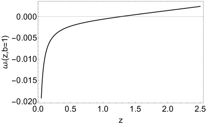
Figure 4: The function $\omega_{o}$ in (76), assuming a concordance model, and with ${\cal Q}=0$, $b=1$ .

In Fig. 5 we plot the rocket Kaiser contribution at wide-angle scales of $\xi_{v_{\|o}v_{\|o}}$ at different $z$ and how the contribution in (113) depends on the separation angle $2\theta$. Indeed, it easy to see that for $\theta\to 0$ is constant (as we pointed out in the flat-sky regime) and is zero when $\theta=\pi/4$ because $\mathcal{P}_{1}(\cos(\pi/2))=0$.

Figure 5: Absolute value of the correlation $\xi_{v_{\|o}v_{\|o}}$ as a function of the separation angle $\theta$, for different values of $z_{1}=z_{2}$.

In this section, we ignore the integrated part of $\xi$ and focus on the local part of Eq. (35). Now, in order to understand which local term is more important and in which configuration, we separate the correlation in Eq. (121) in several parts. Precisely, let us divide $\xi$ as follows:

$$\xi=\xi_{{\rm loc}-K}+\xi_{\rm loc-wide}+\xi_{v_{\|o}{\rm loc}}+\xi_{{\rm loc}\;v_{\|o}}+\xi_{v_{\|o}v_{\|o}},$$ (126)

where we have split $\xi_{\rm loc}=\xi_{{\rm loc}-K}+\xi_{\rm loc-wide}$. In particular,

$\xi_{{\rm loc}-K}$ encodes the effect of the matter overdensity $\delta$ and peculiar velocity $\beta$ due to the Kaiser effect. (Here,  the Kaiser effect represents in Kaiser boost, see Kaiser:1987qv ). In general, this is the correlation function that it is considered in most of the literature (in Raccanelli:2013multipoli ; Raccanelli:2013gja is also called $\xi_{\beta}$).

$\xi_{\rm loc-wide}$ includes all terms that receive contributions from all of $\alpha$ and $\gamma$. Therefore it gives both the wide-angle and mode-coupling contributions, and the relativistic corrections due to potential terms to wide-angle effects (see also Bertacca:2012tp ; Raccanelli:2013multipoli ; Raccanelli:2013gja ; Raccanelli:2016avd ).

$\xi_{v_{\|o}v_{\|o}}$ is the main contribution of the Kaiser Rocket effect.

$\xi_{v_{\|o}{\rm loc}}~{}~{}\&~{}~{}\xi_{{\rm loc}\;v_{\|o}}$ describe the correlation of the local terms (i.e. that depend on $\delta$, $\alpha$, $\beta$ and $\gamma$ ) with the dipole.

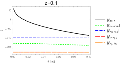
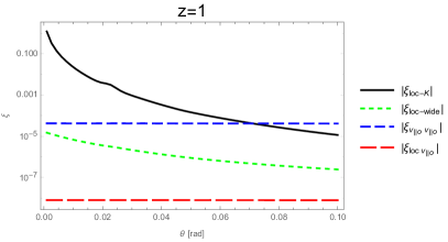
Figure 6: Absolute value of all contributions. Left side with $z_{1}=z_{2}=0.1$, right side with $z_{1}=z_{2}=1$.

The relative importance of the dipole/Rocket effect depends on the particular configuration, i.e. on $\{z_{1},z_{2},\theta\}$. Here below we will study the dependence of these terms for different separation angles, scales, and redshifts of the two galaxies. First of all, let us consider pairs of galaxies transverse to the line of sight, i.e. for $z_{1}=z_{2}$. Fig. 6 shows how the dipole contributions depend on the separation angle $2\theta$. We note that at low redshift, e.g. $z_{1}=z_{2}=0.1$, the contribution $\xi_{{\rm loc}-K}$ is dominant for $\theta<0.1$. Instead, at $z_{1}=z_{2}=1$, $\xi_{v_{\|o}v_{\|o}}>\xi_{{\rm loc}-K}$ for $\theta>0.07$.

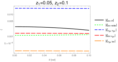
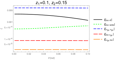
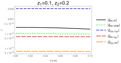
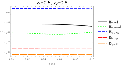
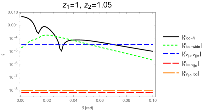
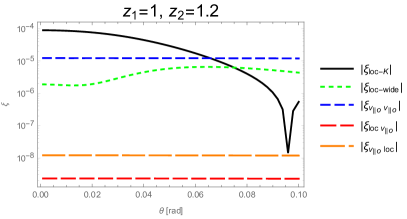
Figure 7: Absolute value of all contributions where we have fixed $z_{1}\neq z_{2}$ and with $\theta$ varying.

In Fig. 7 we still fix $z_{1}$ and $z_{2}$, but with two different values of redshift, galaxies with non-transverse separation. It is clear from the first four panels ( i.e. for $z_{1}=0.05~{}z_{2}=0.1$, $z_{1}=0.1~{}z_{2}=0.15$, $z_{1}=0.1~{}z_{2}=0.2$ and $z_{1}=0.5~{}z_{2}=0.8$) that $\xi_{v_{\|o}v_{\|o}}$ is the dominant contribution of the correlation function on large-scales. In the bottom-left panel, i.e. for $z_{1}=1~{}z_{2}=1.05$, we have a non negligible effect of $\xi_{\rm loc-wide}$ at BAO scales. In general, for most of above panels, $\xi_{\rm loc-wide}$ is subdominant.

Another interesting configuration is to set $\theta$ constant and with $z_{1}=z_{2}$ varying. In Fig. 8 we put $\theta=0.01$rad on the left panel and $\theta=0.1$rad on right panel. As expected for small $\theta$ the dominant contribution here is the standard Kaiser component. Conversely, for large separation angle (e.g. $\theta=0.1$rad), unless around $z=1.3$ [because $\omega_{o}(z=1.3)=0$, e.g. see Fig. 4] the local correlation is weak so the Rocket effect is the only relevant component.

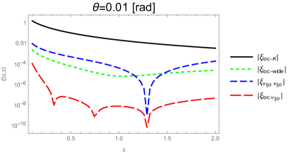
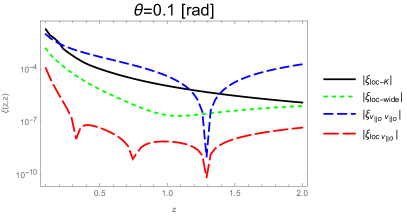
Figure 8: Absolute value of all contributions where we have fixed $\theta$ and with $z=z_{1}=z_{2}$ varying.

Now let us focus on configurations where we fix $z_{1}$ and varying $z_{2}$, both for a small separation angle (see Fig. 9) and for a large separation angle (see Fig. 10). Also in these cases, for distances larger than the Baryon Acoustic Oscillations (BAO) scales the dipole contribution on $\xi$ dominates, as expected.

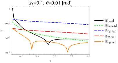
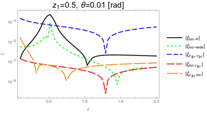
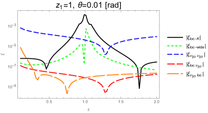
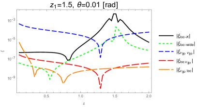
Figure 9: Absolute value of all contributions as a function of $z=z_{2}$, where we have fixed $z_{1}$ and the separation angle $\theta$.

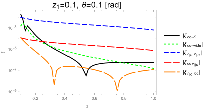
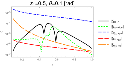
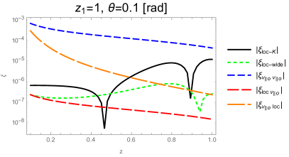
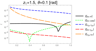
Figure 10: Absolute value of all contributions as a function of $z=z_{2}$, where we have fixed $z_{1}$ and $\theta$ .

As we observe in Eq. (121), the contribution of the Kaiser Rocket effect is mainly in the monopole over the pair orientation angle $\varphi$, i.e. for $\tilde{L}=0$. Therefore, it is useful to focus in detail the corrections to the local correlation function, due to the Rocket effect. Due to the fact that this contribution might be important in wide and deep surveys, we have to consider carefully the geometry of the system. Precisely, we follow the approach suggested in Raccanelli:2013multipoli where the authors introduced a suitable modification in the argument of the Legendre polynomials, i.e. in the angular dependence of the multipole expansion. For the monopole we have to use the following relations

$$\xi_{{\rm loc}0}(z_{2},\theta) = \frac{1}{2}\frac{\pi}{\pi-2\theta}\int_{\theta}^{\pi-\theta}~{}d\varphi~{}\xi_{\rm loc}(z_{2},\theta,\varphi)~{}\mathcal{P}_{0}\left\{\cos\left[\frac{\pi\left(\varphi-\theta\right)}{\pi-2\theta}\right]\right\}\,\rm sin\left[\frac{\pi\left(\varphi-\theta\right)}{\pi-2\theta}\right]\;,$$ (127)

$$\Delta\xi_{0}(z_{2},\theta) = \frac{1}{2}\frac{\pi}{\pi-2\theta}\int_{\theta}^{\pi-\theta}~{}d\varphi~{}\left[\xi(z_{2},\theta,\varphi)-\xi_{\rm loc}(z_{2},\theta,\varphi)\right]~{}\mathcal{P}_{0}\left\{\cos\left[\frac{\pi\left(\varphi-\theta\right)}{\pi-2\theta}\right]\right\}\,\rm sin\left[\frac{\pi\left(\varphi-\theta\right)}{\pi-2\theta}\right]\;,\$$ (128)

where we have defined $\varphi$ in the following way

$$\varphi(z_{1},z_{2},\theta)=\cos^{-1}\left\{\sqrt{\frac{1+\cos 2\theta}{2}}\left[\frac{\chi(z_{1})-\chi(z_{2})}{\chi_{12}(z_{1},z_{2},\theta)}\right]\right\}\;.$$ (129)

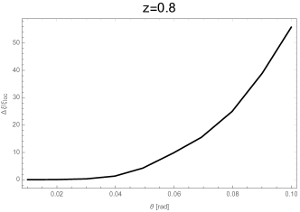
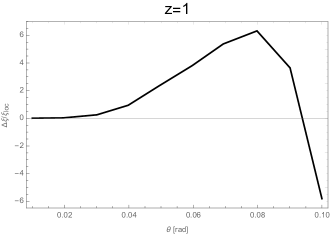
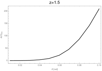
Figure 11: $\Delta\xi_{0}/\xi_{{\rm loc}0}$ as a function of the angular separation $\theta$, for different values of $z_{2}$.

In Fig. 11 we plot $\Delta\xi_{0}/\xi_{{\rm loc}0}$ as a function of the angular separation $\theta$, for different values of $z_{2}$. Also in this case the amplitude of the Rocket effect quickly dominates the local contribution at large angular separations.

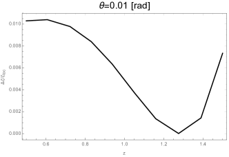
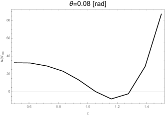
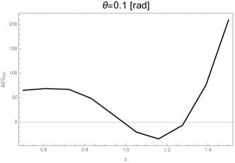
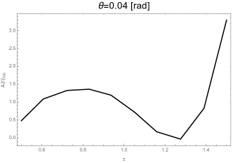
Figure 12: $\Delta\xi_{0}/\xi_{{\rm loc}0}$ as a function of $z_{2}$, for different values of the angular separation $\theta$.

The positive or negative values at large $\theta$ could be motivated by the plots in Fig. 12 where we are showing $\Delta\xi_{0}/\xi_{{\rm loc}0}$ as a function of $z_{2}$, for different values of $\theta$. Precisely, in the bottom-left panel of Fig. 11, we note that $\Delta\xi_{0}/\xi_{{\rm loc}0}$ increases until $\theta\simeq 0.08$ rad and then rapidly decreases into negative values. This curve trend can be explained by the plots in Fig. Ref 5 where $\xi_{v_{\|o}v_{\|o}}$, for $\theta\geq 0.08$ rad, becomes negative. This should produce a maximum for $\Delta\xi_{0}/\xi_{{\rm loc}0}$.

The evaluation of how this impacts on galaxy clustering measurements is beyond the scope of this paper and is left to a future work.

IX Conclusions

In this paper we investigate the wide-angle correlations in the galaxy power spectrum in redshift space, including both all general relativistic effects and the Kaiser Rocket effect (which depends on the dipole of the observer).

We showed via illustrative examples that the Rocket effect on large scales could in principle dominate the local signal of the 2-point correlation function of galaxies at very large scales (see also Scaccabarozzi:2018vux ). As we can see from Figs. 6, 7, 8, 9, 10, 11, 12, the Rocket effect depends on the redshift of the galaxies, the magnification bias $\mathcal{Q}$, the evolution bias $b_{e}$ and the angular separation $2\theta$.

From this work we understood that it is important to evaluate the Kaiser rocket effect well. In particular, it is important to understand if it is only a possible source of systematic effects or, if isolated and measured, it allows us to estimate cosmological parameters and break degenerations. Future wide and deep surveys will need to utilise a more precise modelling, including all geometry, relativistic and the dipole corrections. The next step will be to implement this effect in LIGER Borzyszkowski:2017ayl where, building mock galaxy catalogues including all general relativistic corrections at linear order in the cosmological perturbations, we can quantify the impact and investigate the detectability of the Kaiser Rocket effect in the angular clustering of galaxies from forthcoming survey data.

In addition, for future surveys, it might be important to quantify if the Rocket terms could contaminate $f_{\rm NL}$ constraints and, at the same time, how to disentangle these two effects. Note that the Rocket effects will depend on $\omega_{o}$ (which are proportional to the evolution and the magnification bias). Therefore, it is also useful to study in details the relation between window function/selection function (via $\omega_{o}$) of the surveys and the Rocket effect at different redshift. Finally it is also important to understand if these results are sensitive to the fiducial model. We leave these efforts to a future work.

- (1) A. Kogut et al., Astrophys. J. 419 (1993) 1 doi:10.1086/173453 [astro-ph/9312056].
- (2) A. Yahil, G. A. Tammann and A. Sandage, Astrophys. J. 217 (1977) 903. doi:10.1086/155636
- (3) D. J. Fixsen, E. S. Cheng, J. M. Gales, J. C. Mather, R. A. Shafer and E. L. Wright, Astrophys. J. 473 (1996) 576 doi:10.1086/178173 [astro-ph/9605054].
- (4) G. Hinshaw et al. [WMAP Collaboration], Astrophys. J. Suppl. 180 (2009) 225 doi:10.1088/0067-0049/180/2/225 [arXiv:0803.0732 [astro-ph]].
- (5) C. Gibelyou and D. Huterer, Mon. Not. Roy. Astron. Soc. 427 (2012) 1994 doi:10.1111/j.1365-2966.2012.22032.x [arXiv:1205.6476 [astro-ph.CO]].
- (6) A. Nusser, M. Davis and E. Branchini, Astrophys. J. 788 (2014) 157 doi:10.1088/0004-637X/788/2/157 [arXiv:1402.6566 [astro-ph.CO]].
- (7) R. Maartens, C. Clarkson and S. Chen, JCAP 1801 (2018) no.01, 013 doi:10.1088/1475-7516/2018/01/013 [arXiv:1709.04165 [astro-ph.CO]].
- (8) N. Pant, A. Rotti, C. A. P. Bengaly and R. Maartens, JCAP 1903 (2019) 023 doi:10.1088/1475-7516/2019/03/023 [arXiv:1808.09743 [astro-ph.CO]].
- (9) A. Baleisis, O. Lahav, A. J. Loan and J. V. Wall, Mon. Not. Roy. Astron. Soc. 297 (1998) 545 doi:10.1046/j.1365-8711.1998.01536.x [astro-ph/9709205].
- (10) C. Blake and J. Wall, Nature 416 (2002) 150 doi:10.1038/416150a [astro-ph/0203385].
- (11) A. K. Singal, Astrophys. J. 742 (2011) L23 doi:10.1088/2041-8205/742/2/L23 [arXiv:1110.6260 [astro-ph.CO]].
- (12) M. Rubart and D. J. Schwarz, Astron. Astrophys. 555 (2013) A117 doi:10.1051/0004-6361/201321215 [arXiv:1301.5559 [astro-ph.CO]].
- (13) P. Tiwari, R. Kothari, A. Naskar, S. Nadkarni-Ghosh and P. Jain, Astropart. Phys. 61 (2014) 1 doi:10.1016/j.astropartphys.2014.06.004 [arXiv:1307.1947 [astro-ph.CO]].
- (14) D. J. Schwarz et al., PoS AASKA 14 (2015) 032 doi:10.22323/1.215.0032 [arXiv:1501.03820 [astro-ph.CO]].
- (15) P. Tiwari and A. Nusser, JCAP 1603 (2016) 062 doi:10.1088/1475-7516/2016/03/062 [arXiv:1509.02532 [astro-ph.CO]].
- (16) J. Colin, R. Mohayaee, M. Rameez and S. Sarkar, Mon. Not. Roy. Astron. Soc. 471 (2017) no.1, 1045 doi:10.1093/mnras/stx1631 [arXiv:1703.09376 [astro-ph.CO]].
- (17) C. A. P. Bengaly, R. Maartens and M. G. Santos, JCAP 1804 (2018) no.04, 031 doi:10.1088/1475-7516/2018/04/031 [arXiv:1710.08804 [astro-ph.CO]].
- (18) P. J. E., Peebles, “ The large-scale structure of the universe”, Princeton, N.J., Princeton University Press, 1980. 435 p.
- (19) M. Davis, A. Nusser, K. Masters, C. Springob, J. P. Huchra and G. Lemson, Mon. Not. Roy. Astron. Soc. 413 (2011) 2906 doi:10.1111/j.1365-2966.2011.18362.x [arXiv:1011.3114 [astro-ph.CO]].
- (20) M. A. Strauss and J. A. Willick, Phys. Rept. 261 (1995) 271 doi:10.1016/0370-1573(95)00013-7 [astro-ph/9502079].
- (21) R. Juszkiewicz, N. Vittorio, R. F. G. Wyse Astrophys. J. 349 (1990) 408-414
- (22) O. Lahav, N. Kaiser and Y. Hoffman, Astrophys. J. 352 (1990) 448-456 doi:10.1086/168550
- (23) J. A. Peacock, Mon. Not. Roy. Astron. Soc. 258 (1992) 581-586.
- (24) N. Kaiser, Mon. Not. Roy. Astron. Soc. 227 (1987) 1.
- (25) A. J. S. Hamilton, astro-ph/9708102.
- (26) J. Yoo, Phys. Rev. D 79 (2009) 023517 [arXiv:0808.3138 [astro-ph]].
- (27) J. Yoo, A. L. Fitzpatrick and M. Zaldarriaga, Phys. Rev. D 80, 083514 (2009) [arXiv:0907.0707].
- (28) J. Yoo, Phys. Rev. D 82, 083508 (2010) [arXiv:1009.3021].
- (29) C. Bonvin and R. Durrer, Phys. Rev. D 84, 063505 (2011) [arXiv:1105.5280].
- (30) A. Challinor and A. Lewis, Phys. Rev. D 84, 043516 (2011) [arXiv:1105.5292].
- (31) M. Bruni, R. Crittenden, K. Koyama, R. Maartens, C. Pitrou and D. Wands, Phys. Rev. D85 041301 (2012) [arXiv:1106.3999].
- (32) T. Baldauf, U. Seljak, L. Senatore and M. Zaldarriaga, arXiv:1106.5507.
- (33) D. Jeong, F. Schmidt and C. M. Hirata, Phys. Rev. D 85, 023504 (2012) [arXiv:1107.5427].
- (34) J. Yoo, N. Hamaus, U. Seljak and M. Zaldarriaga, arXiv:1109.0998.
- (35) D. Bertacca, R. Maartens, A. Raccanelli and C. Clarkson, JCAP 1210 (2012) 025 [arXiv:1205.5221 [astro-ph.CO]].
- (36) J. Yoo, N. Hamaus, U. Seljak and M. Zaldarriaga, Phys. Rev. D 86 (2012) 063514 [arXiv:1206.5809 [astro-ph.CO]].
- (37) J. Yoo and V. Desjacques, Phys. Rev. D 88 (2013) no.2, 023502 [arXiv:1301.4501 [astro-ph.CO]].
- (38) A. Raccanelli, D. Bertacca, O. Doré and R. Maartens, JCAP 1408 (2014) 022 [arXiv:1306.6646 [astro-ph.CO]].
- (39) E. Di Dio, F. Montanari, J. Lesgourgues and R. Durrer, JCAP 1311 (2013) 044 [arXiv:1307.1459 [astro-ph.CO]].
- (40) J. Yoo and U. Seljak, Mon. Not. Roy. Astron. Soc. 447 (2015) no.2, 1789 [arXiv:1308.1093 [astro-ph.CO]].
- (41) E. Di Dio, F. Montanari, R. Durrer and J. Lesgourgues, JCAP 1401 (2014) 042 [arXiv:1308.6186 [astro-ph.CO]].
- (42) C. Bonvin, L. Hui and E. Gaztanaga, Phys. Rev. D 89 (2014) no.8, 083535 [arXiv:1309.1321 [astro-ph.CO]].
- (43) A. Raccanelli, D. Bertacca, R. Maartens, C. Clarkson and O. Doré, Gen. Rel. Grav. 48 (2016) no.7, 84 [arXiv:1311.6813 [astro-ph.CO]].
- (44) D. J. Bacon, S. Andrianomena, C. Clarkson, K. Bolejko and R. Maartens, Mon. Not. Roy. Astron. Soc. 443 (2014) no.3, 1900 [arXiv:1401.3694 [astro-ph.CO]].
- (45) S. Chen and D. J. Schwarz, Phys. Rev. D 91 (2015) no.4, 043507 doi:10.1103/PhysRevD.91.043507 [arXiv:1407.4682 [astro-ph.GA]].
- (46) A. Raccanelli, F. Montanari, D. Bertacca, O. Doré and R. Durrer, JCAP 1605 (2016) no.05, 009 [arXiv:1505.06179 [astro-ph.CO]].
- (47) D. Alonso, P. Bull, P. G. Ferreira, R. Maartens and M. Santos, Astrophys. J. 814 (2015) no.2, 145 [arXiv:1505.07596 [astro-ph.CO]].
- (48) F. Montanari and R. Durrer, JCAP 1510 (2015) no.10, 070 [arXiv:1506.01369 [astro-ph.CO]].
- (49) S. Chen and D. J. Schwarz, Astron. Astrophys. 591 (2016) A135 doi:10.1051/0004-6361/201526956 [arXiv:1507.02160 [astro-ph.CO]].
- (50) D. Alonso and P. G. Ferreira, Phys. Rev. D 92 (2015) no.6, 063525 doi:10.1103/PhysRevD.92.063525 [arXiv:1507.03550 [astro-ph.CO]].
- (51) J. Fonseca, S. Camera, M. Santos and R. Maartens, Astrophys. J. 812 (2015) no.2, L22 [arXiv:1507.04605 [astro-ph.CO]].
- (52) C. Bonvin, L. Hui and E. Gaztanaga, JCAP 1608 (2016) no.08, 021 [arXiv:1512.03566 [astro-ph.CO]].
- (53) E. Gaztanaga, C. Bonvin and L. Hui, JCAP 1701 (2017) no.01, 032 [arXiv:1512.03918 [astro-ph.CO]].
- (54) W. Cardona, R. Durrer, M. Kunz and F. Montanari, Phys. Rev. D 94 (2016) no.4, 043007 [arXiv:1603.06481 [astro-ph.CO]].
- (55) A. Raccanelli, D. Bertacca, D. Jeong, M. C. Neyrinck and A. S. Szalay, Phys. Dark Univ. 19 (2018) 109 doi:10.1016/j.dark.2017.12.003 [arXiv:1602.03186 [astro-ph.CO]].
- (56) E. Di Dio, F. Montanari, A. Raccanelli, R. Durrer, M. Kamionkowski and J. Lesgourgues, JCAP 1606 (2016) no.06, 013 [arXiv:1603.09073 [astro-ph.CO]].
- (57) M. Borzyszkowski, D. Bertacca and C. Porciani, Mon. Not. Roy. Astron. Soc. 471 (2017) no.4, 3899 doi:10.1093/mnras/stx1423 [arXiv:1703.03407 [astro-ph.CO]].
- (58) F. Scaccabarozzi and J. Yoo, JCAP 1706 (2017) no.06, 007 doi:10.1088/1475-7516/2017/06/007 [arXiv:1703.08552 [gr-qc]].
- (59) L. R. Abramo and D. Bertacca, Phys. Rev. D 96 (2017) no.12, 123535 doi:10.1103/PhysRevD.96.123535 [arXiv:1706.01834 [astro-ph.CO]].
- (60) F. Scaccabarozzi, J. Yoo and S. G. Biern, JCAP 1810 (2018) no.10, 024 doi:10.1088/1475-7516/2018/10/024 [arXiv:1807.09796 [astro-ph.CO]].
- (61) V. Tansella, C. Bonvin, R. Durrer, B. Ghosh and E. Sellentin, JCAP 1803 (2018) no.03, 019 [arXiv:1708.00492 [astro-ph.CO]].
- (62) F. Lepori, E. Di Dio, E. Villa and M. Viel, JCAP 1805 (2018) no.05, 043 doi:10.1088/1475-7516/2018/05/043 [arXiv:1709.03523 [astro-ph.CO]].
- (63) E. Villa, E. Di Dio and F. Lepori, JCAP 1804 (2018) no.04, 033 doi:10.1088/1475-7516/2018/04/033 [arXiv:1711.07466 [astro-ph.CO]].
- (64) V. Tansella, C. Bonvin, G. Cusin, R. Durrer, M. Kunz and I. Sawicki, Phys. Rev. D 98 (2018) no.10, 103515 [arXiv:1807.00731 [astro-ph.CO]].
- (65) N. Schöneberg, M. Simonović, J. Lesgourgues and M. Zaldarriaga, JCAP 1810 (2018) 047 [arXiv:1807.09540 [astro-ph.CO]].
- (66) V. Tansella, G. Jelic-Cizmek, C. Bonvin and R. Durrer, JCAP 1810 (2018) 032 [arXiv:1806.11090 [astro-ph.CO]].
- (67) M. A. Breton, Y. Rasera, A. Taruya, O. Lacombe and S. Saga, Mon. Not. Roy. Astron. Soc. 483 (2019) no.2, 2671 [arXiv:1803.04294 [astro-ph.CO]].
- (68) A. Yahil, M. A. Strauss, M. Davis and J. P. Huchra, Astrophys. J. 372 (1991) 380-393, doi:10.1086/169985
- (69) M. Davis, M. A. Strauss, and A. Yahil, Astrophys. J. 372 (1991) 394-409, doi:10.1086/169986
- (70) K. B. Fisher, O. Lahav, Y. Hoffman, D. Lynden-Bell and S. Zaroubi, Mon. Not. Roy. Astron. Soc. 272 (1995) 885.
- (71) A. Nusser and M. Davis, Astrophys. J. 421 (1994) L1 doi:10.1086/187172 [astro-ph/9309009].
- (72) A. Nusser, E. Branchini and M. Davis, Astrophys. J. 744 (2012) 193 doi:10.1088/0004-637X/744/2/193 [arXiv:1106.6145 [astro-ph.CO]].
- (73) C. P. Ma and E. Bertschinger, Astrophys. J. 455 7 (1995) [arXiv:astro-ph/9506072].
- (74) S. Matarrese, S. Mollerach and M. Bruni, Phys. Rev. D 58 043504 (1998) [arXiv:astro-ph/9707278].
- (75) F. Schmidt, E. Rozo, S. Dodelson, L. Hui and E. Sheldon, Phys. Rev. Lett. 103, 051301 (2009) doi:10.1103/PhysRevLett.103.051301 [arXiv:0904.4702 [astro-ph.CO]].
- (76) F. B. Abdalla and S. Rawlings, Mon. Not. Roy. Astron. Soc. 360, 27 (2005) doi:10.1111/j.1365-2966.2005.08650.x [astro-ph/0411342].
- (77) A. Hall, C. Bonvin and A. Challinor, Phys. Rev. D 87, no. 6, 064026 (2013) doi:10.1103/PhysRevD.87.064026 [arXiv:1212.0728 [astro-ph.CO]].
- (78) A. S. Szalay, T. Matsubara and S. D. Landy, astro-ph/9712007.
- (79) S. Bharadwaj, Astrophys. J. 516 (1999) 507 [astro-ph/9812274].
- (80) T. Matsubara, astro-ph/9908056.
- (81) I. Szapudi, Astrophys. J. 614 51 (2004) [astro-ph/0404477].
- (82) P. Papai and I. Szapudi, arXiv:0802.2940.
- (83) A. Raccanelli, L. Samushia and W. J. Percival, arXiv:1006.1652.
- (84) L. Samushia, W. J. Percival and A. Raccanelli, arXiv:1102.1014.
- (85) N. Aghanim et al. [Planck Collaboration], arXiv:1807.06209 [astro-ph.CO].