An Efficient Augmented Lagrangian Method for Support Vector Machine

Abstract

Abstract. Support vector machine (SVM) has proved to be a successful approach for machine learning. Two typical SVM models are the L1-loss model for support vector classification (SVC) and $\epsilon$-L1-loss model for support vector regression (SVR). Due to the nonsmoothness of the L1-loss function in the two models, most of the traditional approaches focus on solving the dual problem. In this paper, we propose an augmented Lagrangian method for the L1-loss model, which is designed to solve the primal problem. By tackling the non-smooth term in the model with Moreau-Yosida regularization and the proximal operator, the subproblem in augmented Lagrangian method reduces to a non-smooth linear system, which can be solved via the quadratically convergent semismooth Newton’s method. Moreover, the high computational cost in semismooth Newton’s method can be significantly reduced by exploring the sparse structure in the generalized Jacobian. Numerical results on various datasets in LIBLINEAR show that the proposed method is competitive with the most popular solvers in both speed and accuracy.

1 Introduction

Support vector machine (SVM) has proved to be a successful approach for machine learning. Support vector classification (SVC) and support vector regression (SVR) are two main types of support vector machines (SVMs). Support vector classification is a classic and well-performed learning method for two-group classification problems [7], whereas support vector regression is a learning machine extended from SVC by Boser et al. [2]. Given a training dataset, the learning algorithms for SVC can be used to find a maximum-margin hyperplane that divides all the training examples into two categories. It obtains the prediction function based on only a subset of support vectors. For SVR, instead of minimizing the training error, support vector regression minimizes the generalization error bound [1] with a maximum-tolerance $\epsilon$, below which we do not have to compute the loss. Two typical models are the L1-loss SVC model and the $\epsilon$-L1-loss SVR model.

For L1-loss SVC, due to the nonsmoothness of the hinge loss function, traditional ways to deal with the hinge loss function is to introduce slack variables to formulate the problem as an optimization problem with a smooth function and linear inequality constraints. Most approaches are proposed to solve the dual problem. For example, Platt [27] presented a sequential minimal optimization (SMO) algorithm. It deals with the dual problem by breaking the large quadratic programming(QP) optimization problem into a series of small quadratic programming problems. The fast APG (FAPG) method [14] is another widely used method to solve the QP problem with linear and bounds constraints. Joachims proposed ${\rm SVM^{light}}$ [15] and ${\rm SVM^{perf}}$ [16] respectively. ${\rm SVM^{light}}$ is based on a generalized version of the decomposition strategy. In each iteration, all the variables of the dual problem are divided into two sets. One is the set of free variables and the other is the set of fixed variables. ${\rm SVM^{perf}}$ uses a cutting-plane algorithm for training structural classification SVMs and ordinal regression SVMs. Smola et al. [36] improved ${\rm SVM^{perf}}$ by applying bundle methods and it performed well for large-scale data sets. An exponentiated gradient (EG) method was proposed by Collins et al. [6]. The EG method is based on exponentiated gradient updates and can be used to solve both the log-linear and max-margin optimization problems. Hsieh et al. [13] proposed a dual coordinate descent (DCD) method for linear SVM to deal with large-scale sparse data. Methods aiming to solve the primal form of the problem include the stochastic gradient descent method (SGD) and its different variants such as averaged SGD (ASGD) [47]. Shalev-Shwartz et al. [34] proposed the Pegasos algorithm by introducing subgradient of the approximation for the objective function to cope with the non-differentiability of the hinge loss function. They considered a different procedure for setting the step size and included gradient-projection approach as an optional step. NORMA method proposed by Kivinen et al. [18] is also a variant of stochastic subgradient method based on the kernel expansion of the function. Inspired by Huber loss, Chapelle [3] used a differentiable approximation of L1-loss function. Tak${\rm\acute{a}\check{c}}$ et al. [42] introduced the mini-batch technique in Pegasos algorithm to guarantee the parallelization speedups. Recently, Chauhan et al. [4] presented a review on linear SVM and concluded that SVM-ALM proposed by Nie [25] was the fastest algorithm which was applied to the L_p-loss primal problem by introducing the augmented Lagrangian method, and LIBLINEAR [9] is the most widely used solver which applied DCD to solving L2-regularized dual SVM. Niu et al. [26] proposed SSsNAL method to solve the large-scale SVMs with big sample size by using the augmented Lagrangian method to deal with the dual problem.

For the $\epsilon$-L1-loss SVR model, similar to SVC, a new dual coordinate descent (DCD) method was proposed by Ho and Lin [12] for linear SVR. Burges et al. [8] applied an active set method to solving the dual quadratic programming problem. Smola [35] introduced a primal-dual path method to solve the dual problem. Similarly, stochastic gradient descent methods have good performance in solving large-scale support vector regression problem.

On the other hand, in optimization community, there are some recent progress on methodologies and techniques to deal with non-smooth problems. A typical tool is the semismooth Newton method, which is to solve non-smooth linear equations [31]. Semismooth Newton’s method has been successfully applied in solving various model optimization problems including nearest correlation matrix problem [29], nearest Euclidean distance matrix problem [28], and so on [17, 19, 30]. Moreover, Zhong and Fukushima [50] use semismooth Newton’s method to solve the multi-class support vector machines. Recently, it is used to solve L2-loss SVC and $\epsilon$-L2-loss SVR [44]. For optimization problems including non-smooth terms in objective functions, Sun and his collaborators proposed different approaches based on the famous Moreau-Yosida regularization. For example, to deal with the well-known LASSO problems, a highly efficient semismooth Newton augmented Lagrangian method is proposed in [20]. Similar technique is used to solve the OSCAR and SLOPE models, as well as convex clustering [22, 39]. To deal with two non-smooth terms in objective functions, an ABCD (accelerated block coordinate descent) framework [38] is proposed with the symmetric Gauss-Seidel technique embedded. The ABCD approach was applied to solve the Euclidean distance matrix model for protein molecular conformation in [46]. In fact, the augmented Lagrangian method is quite popular and powerful to solve constraint optimization problems. With semismooth Newton’s method as a subsolver, it is able to deal with various problems with non-smooth terms. The famous SDPNAL+ [48, 49, 43, 40] is designed under the framework of augmented Lagrangian method.

Based on the above observations, a natural question arises. Given the fact that semismooth Newton’s method has been used to solve L2-loss SVC and SVR, is it possible to solve the corresponding L1-loss models by making use of the modern optimization technique and approaches to tackle the non-smooth term? It is this question that motivates the work in our paper.

The contribution of the paper is as follows. Firstly, we propose an augmented Lagrangian method to solve the primal form of the L1-loss model for SVC and $\epsilon$-L1-loss model for SVR. The challenge of the nonsmoothness is tackled with Moreau-Yosida regularization. Secondly, we apply semismooth Newton’s method to solve the resulting subproblem. The quadratic convergence rate for semismooth Newton’s method is guaranteed. Moreover, by exploring the sparse structure of the generalized Jacobian, the high computational complexity for semismooth Newton’s method can be significantly reduced. Finally, extensive numerical tests and datasets in LIBLINEAR demonstrate the fast speed and impressive accuracy of the method.

The organization of the paper is as follows. In Section 2, we introduce the two models for SVM, i.e., L1-loss SVC and $\epsilon$-L1-loss SVR, and give some preliminaries. In Section 3, we apply the augmented Lagrangian method to solve the L1-loss SVC model. In Section 4, we discuss the semismooth Newton method for subproblem as well as the computational complexity and convergence rate. In Section 5, we apply the above framework to the $\epsilon$-L1-loss SVR model. Numerical results are reported in Section 6 to show the efficiency of the proposed method. Final conclusions are given in Section 7.

Notations. We use $\|\cdot\|$ to denote the $l_{2}$ norm for vectors and Frobenius norm for matrices. $\|x\|_{1}$ is the $l_{1}$ norm for vector $x$ and $\|x\|_{\infty}$ is the infinite norm of $x$. $|\Omega|$ denotes the number of elements in set $\Omega$ and $|a|$ denotes the absolute value of the real number $a$. Let $\mathcal{S}^{n}$ be the set of symmetric matrices. We use $A\succeq 0$ ($A\succ 0$) to mean that $A\in\mathcal{S}^{n}$ is positive semidefinite (positive definite). Let $\hbox{Diag}(u)$ denote a diagonal matrix with diagonal elements coming from vector $u\in\mathbb{R}^{m}$. We use $p^{*}(\cdot)$ to denote the Fenchel conjugate of a function $p(\cdot)$.

2 Problem statement and preliminaries

In this section, we will briefly describe two models for SVM and give some preliminaries including Danskin theorem, semismoothness and proximal mapping.

2.1 Two models for SVM

2.1.1 The L1-loss SVC model

Given training data $(x_{i},y_{i}),\ i=1,\dots m$, where $x_{i}\in\mathbb{R}^{n}$ are the observations, $y_{i}\in\{-1,1\}$ are the labels, the support vector classification is to find a hyperplane $y=w^{T}x+b$ such that the data with different labels can be separated by the hyperplane. The typical SVC model is

$$\begin{split}\min_{\omega\in\mathbb{R}^{n},\ b\in\mathbb{R}}&\ \ \frac{1}{2}\|\omega\|^{2}\\ \hbox{s.t.}\ \ \ \ \ &y_{i}(\omega^{T}x_{i}+b)\geq 1,\ i=1,\dots,\ m.\end{split}$$ (1)

Model (1) is based on the assumption that the two types of data can be successfully separated by the hyperplane. However, in practice, this is usually not the case. A more practical and popular model is the regularized penalty model

$$\min_{\omega\in\mathbb{R}^{n},\ b\in\mathbb{R}}\\ \ \frac{1}{2}\|\omega\|^{2}+C\sum_{i=1}^{m}\xi(\omega;x_{i},y_{i},b),$$ (2)

where $C>0$ is a penalty parameter and $\xi(\cdot)$ is the loss function. Three frequently used loss functions are as follows.

• L1-loss or $l_{1}$ hinge loss: $\xi(\omega;x_{i},y_{i},b)=\max(1-y_{i}(\omega^{T}x_{i}+b),0)$;

• L2-loss or squared hinge loss: $\xi(\omega;x_{i},y_{i},b)=\max(1-y_{i}(\omega^{T}x_{i}+b),0)^{2}$;

• Logistic loss: $\xi(\omega;x_{i},y_{i},b)=\log(1+e^{-y_{i}(\omega^{T}x_{i}+b)})$.

As mentioned in Introduction, the L2-loss model has already been solved by semismooth Newton’s method in [44]. In our paper, we focus on the L1-loss SVC model, i.e.,

$$\min_{\omega\in\mathbb{R}^{n},b\in\mathbb{R}}\ \frac{1}{2}\|\omega\|^{2}+C\sum_{i=1}^{m}\max(1-y_{i}(\omega^{T}x_{i}+b),0).$$ (3)

Notice that there is a bias term $b$ in the standard SVC model. For large-scale SVC, the bias term is often omitted [12, 13]. By setting

$$x_{i}\longleftarrow[x_{i},1],\ \ \omega\longleftarrow[\omega,b],$$

we reach the following model (referred as L1-Loss SVC [13])

$$\min_{\omega\in\mathbb{R}^{n}}\frac{1}{2}\|\omega\|^{2}+C\sum_{i=1}^{m}\max(1-y_{i}(\omega^{T}x_{i}),0).\\$$ (4)

Mathematically, there is significant difference between problem (3) and problem (4), since problem (3) is convex and problem (4) is strongly convex. On the other hand, it is shown in [12] that the bias term hardly affects the performance in most data (See section 4.5 in [12] for the numerical comparison with and without bias term). As a result, in our paper, we will focus on the unbiased model (4), which enjoys nice theoretical properties.

2.1.2 The $\epsilon$-L1-loss SVR model

Given training data $(x_{i},y_{i}),\ i=1,\dots,m$, where $x_{i}\in\mathbb{R}^{n}$, $y_{i}\in\mathbb{R}$, SVR is to find $\omega\in\mathbb{R}^{n}$ and $b\in\mathbb{R}$ such that $\omega^{T}x_{i}+b$ is close to the target value $y_{i}$, $i=1,\dots,m$. The $\epsilon$-L1-loss SVR model is as follows

$$\min_{\omega\in\mathbb{R}^{n}}\frac{1}{2}\|\omega\|^{2}+C\sum_{i=1}^{m}\max(|\omega^{T}x_{i}-y_{i}|-\epsilon,0),\\$$ (5)

where $\epsilon>0$ and $C>0$ are given parameters. We refer to (5) as $\epsilon$-L1-loss SVR as in [10].

2.2 Preliminaries

2.2.1 Semismoothness

The concept of semismoothness was introduced by Mifflin [23] for functionals. It was extended to vector-valued functions by Qi and Sun [31]. Let $\mathcal{X}$ and $\mathcal{Y}$ be two real finite dimensional Euclidean spaces with an inner product $\langle\cdot,\cdot\rangle$ and its induced norm $\|\cdot\|$ on $\mathcal{X}$.

Definition 2.1.

(Semismoothness [23, 31, 37]). Let $\Phi:\mathcal{O}\subset\mathcal{X}\to\mathcal{Y}$ be a locally Lipschitz continuous function on the open set $\mathcal{O}$. We say that $\Phi$ is semismooth at $x$ if (i) $\Phi$ is directional differentiable at $x$ and (ii) for any $V\in\partial\Phi(x+h)$,

$$\Phi(x+h)-\Phi(x)-Vh=o(\|h\|),\ h\to 0.$$

Here $\partial\Phi(x+h)$ is the Clarke subdifferential [5] of $\Phi$ at $x+h$. $\Phi$ is said to be strongly semismooth at $x$ if $\Phi$ is semismooth at $x$ and for any $V\in\partial\Phi(x+h)$,

$$\Phi(x+h)-\Phi(x)-Vh=O(\|h\|^{2}),\ h\to 0.$$

It is easy to check that piecewise linear functions are strongly semismooth. Furthermore, the composition of (strongly) semismooth functions is also (strongly) semismooth. A typical example of strongly semismooth function is $\max(0,t),\ t\in\mathbb{R}$.

2.2.2 Moreau-Yosida regularization

Let $q:\mathcal{X}\longrightarrow(-\infty,+\infty)$ be a closed convex function. The Moreau-Yosida [24, 45] regularization of $q$ at $x\in\mathcal{X}$ is defined by

$$\theta_{q}(x):=\min_{y\in\mathcal{X}}\frac{1}{2}\|y-x\|^{2}+q(y).$$ (6)

The unique solution of (6), denoted as $\hbox{Prox}_{q}(x)$, is called the proximal point of $x$ associated with $q$. The following property holds for Moreau-Yosida regularization [21, Proposition 2.1].

Proposition 2.2.

Let $q:\mathcal{X}\longrightarrow(-\infty,+\infty)$ be a closed convex function, $\theta(\cdot)$ be the Moreau-Yosida regularization of $q$ and $\hbox{Prox}_{q}(\cdot)$ be the associated proximal point mapping. Then $\theta_{q}(\cdot)$ is continuously differentiable, and there is

$$\nabla\theta_{q}(x)=x-\hbox{Prox}_{q}(x).$$

Let

$$p(s)=C\sum_{i=1}^{m}\max(s_{i},0),\ s\in\mathbb{R}^{m}.$$ (7)

The proximal mapping, denoted as $\hbox{Prox}_{p}^{M}(\cdot)$, is defined as the solution of the following problem

$$\phi(z):=\min_{s\in\mathbb{R}^{m}}\psi(z,s),$$ (8)

where $\psi(z,s):=\frac{1}{2M}\|z-s\|^{2}+p(s),\ z\in\mathbb{R}^{m}.$ It is easy to derive that $\hbox{Prox}_{p}^{M}(z)$ takes the following form (See Appendix for the details of deriving $\hbox{Prox}_{p}^{M}(z)$)

$$(\hbox{Prox}_{p}^{M}(z))_{i}=\left\{\begin{array}[]{ll}z_{i}-CM,&z_{i}>CM,\\ z_{i},&z_{i}<0,\\ 0,&0\leq z_{i}\leq CM.\end{array}\right.$$ (9)

The proximal mapping $\hbox{Prox}_{p}^{M}(\cdot)$ is piecewise linear as shown in Figure 2, and therefore strongly semismooth.

Remark 2.3.

Here we would like to point out that the proximal mapping here is closely related to the proximal mapping associate with $\|s\|_{1}$, which is popular used in the well-known LASSO problem. Actually, from Figure 2 and Figure 2, the proximal mapping $\hbox{Prox}_{p}^{M}(\cdot)$ can be viewed as a shift of that with $\|s\|_{1}$.

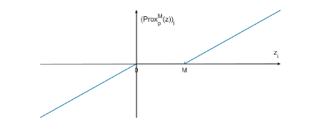
Figure 1: Demonstration of $\hbox{Prox}_{p}^{M}(z_{i})$

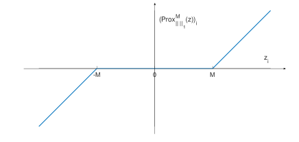
Figure 2: Demonstration of $\hbox{Prox}_{\|\cdot\|_{1}}^{M}(z_{i})$

Given $z$, the Clarke subdifferential of $\hbox{Prox}_{p}^{M}(z)$, denoted as $\partial\hbox{Prox}_{p}^{M}(z)$, is a set of diagonal matrices. For $U\in\partial\hbox{Prox}_{p}^{M}(z)$, its diagonal elements take the following form

$$U_{ii}=\left\{\begin{array}[]{ll}1,&z_{i}>CM,\hbox{ or }z_{i}<0,\\ 0,&0<z_{i}<CM,\\ {u_{i},\ 0\leq u_{i}\leq 1},&z_{i}=0,\hbox{ or }z_{i}=CM.\end{array}\right.$$ (10)

In other words, we have

$$\partial\hbox{Prox}_{p}^{M}(z) = \big{\{}\hbox{Diag}(u):\ u\in\mathbb{R}^{m},u_{i}=1,\hbox{ if }z_{i}>CM\hbox{ or }z_{i}<0;$$

$${u_{i}=0,\hbox{ if }0<z_{i}<CM;\ u_{i}\in[0,1],\ \hbox{otherwise}}\big{\}}.$$

Similarly, for $p_{\epsilon}(\cdot)$ defined by

$$p_{\epsilon}(s)=C\sum_{i=1}^{m}\max(0,|s_{i}|-\epsilon),$$ (11)

there is (see Figure 3 for ${\rm Prox}_{p_{\epsilon}}^{M}(z)$)

$$({\rm Prox}_{p_{\epsilon}}^{M}(z))_{i}=\left\{\begin{array}[]{ll}z_{i}-CM,&z_{i}\geq\epsilon+CM,\\ \epsilon,&\epsilon<z_{i}<\epsilon+CM,\\ z_{i},&|z_{i}|\leq\epsilon,\\ -\epsilon,&-\epsilon-CM<z_{i}<-\epsilon,\\ z_{i}+M,&z_{i}\leq-\epsilon-CM.\end{array}\right.$$

It can be easily verified that $\partial{\rm Prox}^{M}_{p_{\epsilon}}(z)$ is strongly semismooth as well. For $U\in\partial{\rm Prox}^{M}_{p_{\epsilon}}(z)$, its diagonal elements are given by

$$U_{ii}=\left\{\begin{array}[]{ll}1,&|z_{i}|>\epsilon+CM,{\hbox{ or }|z_{i}|<\epsilon},\\ 0,&\epsilon<|z_{i}|<\epsilon+CM,\\ {u_{i},\ 0\leq u_{i}\leq 1,}&|z_{i}|=\epsilon+CM,\ \hbox{ or }|z_{i}|=\epsilon.\\ \end{array}\right.$$

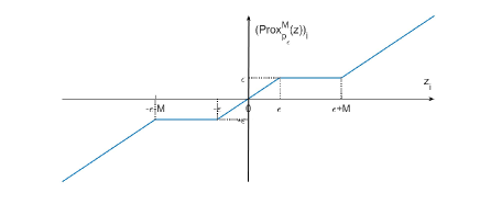
Figure 3: Demonstration of ${\rm Prox}_{p_{\epsilon}}^{M}(z_{i})$

We end this section by the the following property of $p(\cdot)$.

Proposition 2.4.

Let

$$P=\{x\in\mathbb{R}^{m}\ |\ \|x-\frac{C}{2}e\|_{\infty}\leq\frac{C}{2}\},$$

where $e=(1,\dots,1)^{T}\in\mathbb{R}^{m}$. Then we have

$$p(\cdot)=\delta_{P}^{*}(\cdot).$$

Proof. Note that $p(\cdot)$ can be equivalently written as

$$p(s)=\frac{C}{2}s^{T}e+\frac{C}{2}\|s\|_{1}.$$

By the definition of Fenchel conjugate function, there is

$$p^{*}(y) = \sup_{s\in\mathbb{R}^{m}}s^{T}y-p(s)$$

$$= \sup_{s\in\mathbb{R}^{m}}s^{T}y-\frac{C}{2}s^{T}e-\frac{C}{2}\|s\|_{1}$$

$$= \sup_{s\in\mathbb{R}^{m}}s^{T}(y-\frac{C}{2}e)-\frac{C}{2}\|s\|_{1}$$

$$= \frac{C}{2}\sup_{s\in\mathbb{R}^{m}}\frac{2}{C}s^{T}(y-\frac{C}{2}e)-\|s\|_{1}$$

$$:= \frac{C}{2}\sup_{s\in\mathbb{R}^{m}}\frac{2}{C}s^{T}(y-\frac{C}{2}e)-u(s)\quad\ (u(s):=\|s\|_{1})$$

$$= \frac{C}{2}u^{*}(\frac{2}{C}(y-\frac{C}{2}e)).$$

Note that $u^{*}(\cdot)=\delta_{P_{0}}(\cdot)$, where $P_{0}:=\{x\in\mathbb{R}^{m}\ |\ \|x\|_{\infty}\leq 1\}$, and $\delta_{P_{0}}(\cdot)$ is the indicator function defined as $0$ if $x\in P_{0}$ and $+\infty$ otherwise. We then have

$$p^{*}(y)=\frac{C}{2}\delta_{P_{0}}(\frac{2}{C}(y-\frac{C}{2}e))=\delta_{P_{0}}(\frac{2}{C}(y-\frac{C}{2}e))=\delta_{P}(y).$$

In other words, there is $p(\cdot)=\delta_{P}^{*}(\cdot)$. The proof is finished. $\Box$

Proposition 2.5.

Let $\overline{P}:=\{x\in\mathbb{R}^{m}:\|x\|_{\infty}\leq C\}$. There is

$$p_{\epsilon}^{*}(y)=\left\{\begin{array}[]{ll}{\epsilon\|y\|_{1},}&{y\in\overline{P},}\\ {+\infty,}&{\text{otherwise}.}\end{array}\right.$$

Proof. Similar to the proof of Proposition 2.4, there is

$$p_{\epsilon}^{*}(y) = \sup_{x\in\mathbb{R}^{m}}x^{T}y-C\sum_{i=1}^{m}\max(0,|x_{i}|-\epsilon)$$

$$= \sum_{i=1}^{m}\sup_{x_{i}\in\mathbb{R}}x_{i}y_{i}-C\max(0,|x_{i}|-\epsilon).$$

Note that

$$x_{i}y_{i}-C\max(0,|x_{i}|-\epsilon)=\left\{\begin{array}[]{ll}{x_{i}y_{i},}&{\left|x_{i}\right|\leq\epsilon,}\\ {x_{i}\left(y_{i}-C\right)+C\epsilon,}&{x_{i}>\epsilon,}\\ {x_{i}\left(y_{i}+C\right)+C\epsilon,}&{x_{i}<-\epsilon.}\end{array}\right.$$

We consider the following different cases of $y_{i}$:

• if $|y_{i}|=C$, there is $\sup_{x_{i}}x_{i}y_{i}-C\max(0,|x_{i}|-\epsilon)=C\epsilon$;

• if $|y_{i}|<C$, there is $\sup_{x_{i}}x_{i}y_{i}-C\max(0,|x_{i}|-\epsilon)=|y_{i}|\epsilon$;

• if $|y_{i}|>C$, $\sup_{x_{i}}x_{i}y_{i}-C\max(0,|x_{i}|-\epsilon)=+\infty$.

To sum up, we have

$$\sup_{x_{i}\in\mathbb{R}}x_{i}y_{i}-C\max(0,|x_{i}|-\epsilon)=\left\{\begin{array}[]{ll}{|y_{i}|\epsilon,}&{|y_{i}|\leq C,}\\ {+\infty,}&{|y_{i}|>C.}\end{array}\right.$$

Consequently, we get

$$p_{\epsilon}^{*}(y)=\left\{\begin{array}[]{ll}{\epsilon\|y\|_{1},}&{\|y\|_{\infty}\leq C,}\\ {+\infty,}&{\text{otherwise}.}\end{array}\right.$$

The proof is finished. $\Box$

3 The augmented Lagrangian method

In this section, we will discuss the augmented Lagrangian method to solve the L1-loss SVC model (4).

3.1 Problem reformulation

We first reformulate (4) equivalently as the following form

$$\min_{w\in\mathbb{R}^{n}}\frac{1}{2}\|w\|^{2}+C\|\max(0,Bw+d)\|_{1}$$ (12)

by letting

$$B=-\left[\begin{array}[]{c}y_{1}x_{1}^{T}\\ \vdots\\ y_{m}x_{m}^{T}\end{array}\right]\in\mathbb{R}^{m\times n},\ d=\left[\begin{array}[]{c}1\\ \vdots\\ 1\end{array}\right]\in\mathbb{R}^{m}.$$

By introducing a variable $s\in\mathbb{R}^{m}$, we get the following constrained optimization problem

$$\min_{w\in\mathbb{R}^{n},{s\in\mathbb{R}^{m}}} \ \frac{1}{2}\|w\|^{2}+p(s)$$ (13)

s.t. $$\ s=Bw+d.$$

where $p(s)$ is defined as in (7). The Lagrangian function for (13) is

$$l(w,s,\lambda)=\frac{1}{2}\|w\|^{2}+p(s)-\langle\lambda,s-Bw-d\rangle,$$

where $\lambda\in\mathbb{R}^{m}$ is the Lagrange multiplier corresponding to the equality constraints. The dual problem is

$$\max_{\lambda\in\mathbb{R}^{m}}\ -f(\lambda):=-\frac{1}{2}\|B^{T}\lambda\|^{2}+\left\langle\lambda,d\right\rangle-p^{*}(\lambda).$$ (14)

The KKT conditions associated with problem (13) are given by

$$\left\{\begin{array}[]{ll}s=Bw+d,\\ w+B^{T}\lambda=0,\\ 0\in\partial p(s)-\lambda.\end{array}\right.$$ (15)

Remark 3.1.

It is easy to see that both (13) and (14) admit feasible solutions. Consequently, both (13) and (14) admit optimal solutions. By Theorem 2.1.8 in [41], there is no duality gap between (13) and (14). Moreover, by Theorem 2.1.7 in [41], $(s^{*},w^{*},\lambda^{*})$ solves (15) if and only if $(s^{*},w^{*})$ is an optimal solution to (13) and $\lambda^{*}$ is an optimal solution of (14). Consequently, the set of Lagrange multipliers is not empty.

Remark 3.2.

We would like to point out that after we finished our paper, we realized that problem (13) is a special case of the general problem considered in [20]. Consequently, as we will show below, it enjoys interesting properties, due to which the convergence results of the augmented Lagrangian method (Theorems 3.5 and 3.9) in our paper directly follows from those in [20].

Proposition 3.3.

Let $(w^{*},s^{*})$ be the optimal solution to problem (13). Then the second order sufficient condition holds at $(w^{*},s^{*})$.

Proof. Assume that $(w^{*},s^{*},\lambda^{*})$ is one of the solutions for the KKT system (15). Note that the effective domain of $p(\cdot)$, denoted as $\hbox{dom}(p)$, is $\mathbb{R}^{m}$, therefore, the tangent cone of $\hbox{dom}(p)$ at $s^{*}$ is $\mathbb{R}^{m}$. That is $T_{\hbox{dom}(p)}(s^{*})=\mathbb{R}^{m}$. As a result, by the definition in [20, (7)], the critical cone associate with (13) at $(w^{*},s^{*})$, denoted by $\mathcal{C}(w^{*},s^{*})$, is as follows

$$\mathcal{C}(w^{*},s^{*})=\left\{(d_{1},d_{2})\in\mathbb{R}^{n}\times\mathbb{R}^{m}\ |\ Bd_{1}-d_{2}=0,\ (w^{*})^{T}d_{1}+p^{\prime}(s^{*};d_{2})=0\right\}.$$

Here, $p^{\prime}(s^{*};d_{2})$ denote the directional derivative of $p$ at $s^{*}$ with respect to $d_{2}$.

Next, we will show that

$$(d_{1},d_{2})\neq 0\Longrightarrow d_{1}\neq 0,\ \forall\ (d_{1},d_{2})\in\mathcal{C}(w^{*},s^{*}).$$ (16)

For contradiction, assume that for any $(d_{1},d_{2})\in\mathcal{C}(w^{*},s^{*})$, $d_{1}=0$. Then $(d_{1},d_{2})\in\mathcal{C}(w^{*},s^{*})$ gives that $d_{2}=Bd_{1}=0$, contradicting with $(d_{1},d_{2})\neq 0$. Consequently, (16) holds.

By the definition in [20, Definition 2.6], the second order sufficient condition holds at $(w^{*},s^{*})$ if

$$\langle d_{1},(\nabla h(w^{*}))^{\prime}d_{1}\rangle>0,\ \forall\ 0\neq(d_{1},d_{2})\in\mathcal{C}(w^{*},s^{*}),\ \hbox{where}\ h(w)=\frac{1}{2}\|w\|^{2}.$$ (17)

By the definition of directional derivative, it is easy to calculate that

$$(\nabla h(w^{*}))^{\prime}d_{1}=\lim_{t\downarrow 0}\frac{w^{*}+td_{1}-w^{*}}{t}=d_{1}.$$

Together with (16), (17) reduces to

$$\langle d_{1},d_{1}\rangle>0,\forall\ d_{1}\neq 0,(d_{1},d_{2})\in\mathcal{C}(w^{*},s^{*}),$$

which obviously holds. The proof is finished. $\Box$

3.2 Augmented Lagrangian method (ALM)

Next, we will apply augmented Lagrangian method (ALM) to solve (13). The augmented Lagrangian function of (13) is

$$L_{\sigma}(w,s;\lambda)=\frac{1}{2}\|w\|^{2}+p(s)-\langle\lambda,s-Bw-d\rangle+\frac{\sigma}{2}\|s-Bw-d\|^{2},$$

where $\sigma>0$.

ALM works as follows. At iteration $k$, solve

$$\min_{w,s}\ L_{\sigma_{k}}(w,s;\lambda^{k})$$ (18)

to get $(w^{k+1},s^{k+1})$. Then update the Lagrange multiplier by

$$\lambda^{k+1}=\lambda^{k}-\sigma_{k}(s^{k+1}-Bw^{k+1}-d),$$

and $\sigma_{k+1}\geq\sigma_{k}$.

The key step in ALM is to solve the subproblem (18). Similar to that in [20], given fixed $\sigma>0$ and $\lambda$, let $(w^{*},s^{*})$ denote the unique solution of subproblem (18). Denote

$$\phi(w):=\min_{s}L_{\sigma}(w,s;\lambda).$$

Note that

$$\min_{s}\ L_{\sigma}(w,s;\lambda)=\frac{1}{2}\|w\|^{2}-\frac{1}{2\sigma}\|\lambda\|^{2}+\sigma\min_{s}\ \frac{1}{2}\|s-z(w)\|^{2}+\frac{1}{\sigma}p(s),$$

where

$$z(w)=Bw+d+\frac{\lambda}{\sigma}.$$

There is

$$\phi(w)=\frac{1}{2}\|w\|^{2}-\frac{1}{2\sigma}\|\lambda\|^{2}+\sigma\tau(z(w)),$$ (19)

where $\tau(z(w)):=\min_{s}\ \frac{1}{2}\|s-z(w)\|^{2}+\frac{1}{\sigma}p(s)$ is the Moreau-Yosida regularization of $\frac{1}{\sigma}p(s)$. Therefore, we can get $(w^{*},s^{*})$ by

$$w^{*} =\arg\min\phi(w),$$ (20)

$$s^{*} =s^{*}(w^{*})=\hbox{Prox}^{1/\sigma}_{p}(z(w^{*})).$$ (21)

Due to the strong convexity and the differentiability of $\phi(w)$ in Proposition 2.2, we will apply semismooth Newton’s method to solve (20) in Section 4. The details of ALM is given in Algorithm 3.4.

Algorithm 3.4.

ALM for L1-loss SVC

• Initialization. $\sigma_{0}>0,\lambda^{0}\in\mathbb{R}^{m};w^{0}\in\mathbb{R}^{n}.$ For $k_{1}=0,1,2,...$

• Solve (20) to get $w^{k+1}$. Then Calculate $s^{k+1}=s^{*}(w^{k+1})$ by (21).

• Update $\lambda^{k+1}=\lambda^{k}-\sigma_{k}(s^{k+1}-Bw^{k+1}-d)$.

• Choose $\sigma_{k+1}$ such that $\sigma_{k}\leq\sigma_{k+1}<+\infty.$ Go to S1.

3.3 Convergence results

To guarantee the global convergence of ALM, the following standard stopping criteria [32, 33] are used in [20] to solve (13) approximately

$$(A)\ \ \Psi_{k}(w^{k+1},s^{k+1})-\inf\Psi_{k}\leq\epsilon^{2}_{k}/2\sigma_{k},\ \sum_{k=0}^{\infty}\epsilon_{k}<+\infty$$

where $\Psi_{k}(w,s):=L_{\sigma_{k}}(w,s,\lambda^{k})$. The global convergence result of ALM was originally from [32, 33]. As we mentioned in Remark 3.2, ALM is applied to solve a general form of (13), i.e., problem (D) in [20], and the convergence result, i.e., Theorem 3.2 in [20] is obtained therein. Therefore, as a special case of the problem (D) in [20], we can get the following global convergence result of Alg. 3.4.

Theorem 3.5.

Let the sequence $\{(w^{k},s^{k},\lambda^{k})\}$ be generated by ALM with stopping criteria (A). Then the sequence $\{\lambda^{k}\}$ is bounded and converges to an optimal solution of (14). Moreover, the sequence $\{(w^{k},s^{k})\}$ is also bounded and converges to the unique optimal solution $(w^{*},s^{*})$ of (13).

Proof. Note that the optimal solution for strongly convex problem (12) exists and it is unique. Consequently, (13) admits a unique solution. By Remark 3.1, the set of Lagrange multiplier is also non-empty. Consequently, by Theorem 3.2 in [20], the result holds. $\Box$

To state the local convergence rate, we need the following stopping criteria which are popular used such as in [39] and [20].

$$(B1)\ \ \Psi_{k}(w^{k+1},s^{k+1})-\inf\Psi_{k}\leq(\delta_{k}^{2}/2\sigma_{k})\|\lambda^{k+1}-\lambda^{k}\|^{2},\ \sum_{k=1}^{\infty}\delta_{k}<+\infty,$$

$$(B2)\ \ \hbox{dist}(0,\partial\Psi_{k}(w^{k+1},s^{k+1}))\leq(\delta^{\prime}_{k}/\sigma_{k})\|\lambda^{k+1}-\lambda^{k}\|,\ \sum_{k=1}^{\infty}\delta_{k}^{\prime}\rightarrow 0.$$

We also need the following definitions. Define the maximal monotone operator $T_{f}$ and $T_{l}$ [32] by

$$T_{f}=\partial f(\lambda),\ T_{l}(w,s,\lambda)=\{(w^{\prime},s^{\prime},\lambda^{\prime})\ |\ (w^{\prime},s^{\prime},-\lambda^{\prime})\in\partial l(w,s,\lambda)\}.$$

Definition 3.6.

Let $F:\mathcal{X}\rightrightarrows\mathcal{Y}$ be a multivalued mapping and $(\widetilde{x},\widetilde{y})\in\hbox{gph}F$, where $\hbox{gph}F$ is the graph of $F$ defined by

$$\hbox{gph}F:=\{(x,y)\in\mathcal{X}\times\mathcal{Y}\ |\ y\in F(x)\}.$$

$F$ is said to be metrically subregular at $\widetilde{x}$ for $\widetilde{y}$ with modulus $\kappa\geq 0$ if there exist neighbourhoods $U$ of $\widetilde{x}$ and $V$ of $\widetilde{y}$ such that

$$\hbox{dist}(x,F^{-1}(\widetilde{y}))\leq\kappa\hbox{dist}(\widetilde{y},F(x)\cap V),\ \forall\ x\in U.$$

Definition 3.7.

Let $F:\mathcal{X}\rightrightarrows\mathcal{Y}$ be a multivalued mapping and $y\in\mathcal{Y}$ satisfy $F^{-1}(y)\neq\emptyset$. $F$ is said to satisfy the error bound condition for the point $y$ with modulus $\kappa\geq 0$ if there exists $\epsilon>0$ such that if $x\in\mathcal{X}$ with $\hbox{dist}(y,F(y))\leq\epsilon$, then

$$\hbox{dist}(x,F^{-1}(y))\leq\kappa\hbox{dist}(y,F(x)).$$

Proposition 3.8.

Let $F:\mathcal{X}\rightrightarrows\mathcal{Y}$ be a ployhedral multifunction. Then $F$ satisfies the error bound condition for any $y\in\mathcal{Y}$ satisfying $F^{-1}(y)\neq\emptyset$ with a common modulus $\kappa\geq 0$.

Now we are ready to give the convergence rate of ALM, which is similar to that in [20, Theorem 3.3].

Theorem 3.9.

Let $\{(w^{k},s^{k},\lambda^{k})\}$ be the infinite sequence generated by ALM with stopping criteria (A) and (B1). The following results hold.

• The sequence $\{\lambda^{k}\}$ converges to $\lambda^{*}$, one of the optimal solutions of (14), and for all $k$ sufficiently large, there is

  $$\hbox{dist}(\lambda^{k+1},\Omega)\leq\beta_{k}\hbox{dist}(\lambda^{k},\Omega),$$

  where $\Omega$ is the set of the optimal solutions of (14) and

  $$\beta_{k}=\frac{a_{f}(a_{f}^{2}+\sigma_{k}^{2})^{-\frac{1}{2}}+2\delta_{k}}{1-\delta_{k}}\to\beta_{\infty}=a_{f}(a_{f}^{2}+\sigma_{\infty}^{2})^{-\frac{1}{2}}<1$$

  as $k\to+\infty$. Moreover, $\{(w^{k},s^{k})\}$ converges to the unique optimal solution $(w^{*},s^{*})$ of (13).

• If the stopping criteria (B2) is also used, then for all $k$ sufficiently large, there is

  $$\|(w^{k+1},z^{k+1})-(w^{*},z^{*})\|\leq\beta^{\prime}_{k}\|\lambda^{k+1}-\lambda^{k}\|,$$

  where $\beta^{\prime}_{k}=a_{l}(1+\delta^{\prime}_{k})/\sigma_{k}\to a_{l}/\sigma_{\infty}$ as $k\to+\infty$.

Proof. (i) We only need to show that $T_{f}$ satisfies the error bound condition for the origin with modulus $a_{f}$. By Definition 2.2.1 in [41], (14) is convex piecewise linear-quadratic programming problem. By [41, Proposition 2.2.4], we know that the corresponding operator $T_{f}$ is polyhedral multivalued function. Therefore, by Proposition 3.8, the error bound condition holds at the origin with modulus $a_{f}$. Following Theorem 3.3 in [20], we proved (i). To show (ii), first note that the second order sufficient condition holds for problem (13) by Proposition 3.3. On the other hand, by Proposition 2.4, $p(\cdot)$ is the support function of a non-empty polyhedral convex set. Consequently, by Theorem 2.7 in [20], $T_{l}$ is metrically subregular at $(w^{*},s^{*},\lambda^{*})$ for the origin. Then by the second part of Theorem 3.3 in [20], (ii) holds. The proof is finished. $\Box$

4 Semismooth Newton’s method for solving (20)

In this section, we will discuss semismooth Newton’s method to solve (20). In the first part, we will give the details of semismooth Newton’s method. In the second part, we will analyse the computational complexity of the key step in semismooth Newton’s method. The third part is devoted to the convergence result.

4.1 Semismooth Newton’s method

Note that $\phi(w)$ defined as in (19) is continuously differentiable. By Proposition 2.2, the gradient $\nabla\phi(w)$ takes the following form

$$\nabla\phi(w)=w+\sigma\nabla\tau(z(w))=w+B^{T}\lambda-\sigma B^{T}(s^{*}(w)-Bw-d),$$ (22)

which is strongly semismooth due to the strongly semismoothness of $s^{*}(w)$. The generalized Hessian of $\phi$ at $\omega$, denoted as $\partial^{2}\phi(\omega)$, satisfies the following condition [5, Proposition 2.3.3, Proposition 2.6.6]: for any $h\in\mathbb{R}^{n}$,

$$\partial^{2}\phi(\omega)(h)\subseteq\hat{\partial}^{2}\phi(\omega)(h),$$

where

$$\hat{\partial}^{2}\phi(\omega)=I+\sigma B^{T}B-\sigma B^{T}\partial\hbox{Prox}^{1/\sigma}_{p}(z(w))B.$$ (23)

Consequently, solving (20) is equivalent to solving the following strongly semismooth equations

$$\nabla\phi(w)=0.$$ (24)

We apply semismooth Newton’s method to solve the non-smooth equations (24). At iteration $k$, we update $w$ by

$$w^{k+1}=w^{k}-(V^{k})^{-1}\nabla\phi(w^{k}),\ V^{k}\in\hat{\partial}^{2}\phi(w^{k}).$$

Below, we use the following well studied globalized version of the semismooth Newton method [29, Algorithm 5.1] to solve (24).

Algorithm 4.1.

A globalized semismooth Newton method

• Given $j:=0$. Choose $\omega^{0},\ \sigma\in(0,\ 1)$, $\rho\in(0,\ 1)$, $\delta>0$, $\eta_{0}>0$ and $\ \eta_{1}>0$.

• Calculate $\nabla\phi(\omega^{j})$. If $\|\nabla\phi(\omega^{j})\|\leq\delta$, stop. Otherwise, go to S2.

• Select an element $V^{j}\in\hat{\partial}^{2}\phi(\omega^{j})$ defined as in (23). Apply conjugate gradient (CG) method [11] to find an approximate solution $d^{j}$ by

  $$V^{j}d^{j}+\nabla\phi(\omega^{j})=0$$ (25)

  such that

  $$\|V^{j}d^{j}+\nabla\phi(\omega^{j})\|\leq\mu_{j}\|\nabla\phi(\omega^{j})\|,$$

  where $\mu_{j}=\min(\eta_{0},\ \eta_{1}\|\nabla\phi(\omega^{j})\|)$.

• Do line search, and let $m_{j}>0$ be the smallest integer such that the following holds

  $$\phi(\omega^{j}+\rho^{m}d^{j})\leq\phi(\omega^{j})+\sigma\rho^{m}\nabla\phi(\omega^{j})^{T}d^{j}.$$

  Let $\alpha_{j}=\rho^{m_{j}}$.

• Let $\omega^{j+1}=\omega^{j}+\alpha_{j}d^{j}$, $j:=j+1$, go to S1.

4.2 Computational complexity

It is well-known that the high computational complexity for semismooth Newton’s method comes from solving the linear system in S2 of Alg. 4.1. As designed in Alg. 4.1, we apply the popular solver conjugate gradient method (CG) to solve the linear system iteratively. Recall that $w\in\mathbb{R}^{n}$, $B\in\mathbb{R}^{m\times n}$. The heavy burden in applying CG is to calculate $Vh$, where $h\in\mathbb{R}^{n}$ is a given vector. Below, we will mainly analyse several ways to implement $Vh$, where

$$V=I+\sigma B^{T}B-\sigma B^{T}UB,\quad U\in\partial\hbox{Prox}^{1/\sigma}_{p}(z(w)).$$

Way I. Calculate $V$ explicitly and then calculate $Vh$.

Way II. Do not save $V$ explicitly. Instead, calculate $Vh$ directly by

$$Vh=h+\sigma B^{T}(Bh)-\sigma B^{T}U(Bh).$$

Note that $U=\hbox{Diag}(u)$ is a diagonal matrix with vector $u\in\mathbb{R}^{m}$. We can explore the diagonal structure, and use the following formula

$$Vh=h+\sigma B^{T}(Bh)-\sigma B^{T}\hbox{Diag}(u)(Bh).$$ (26)

Specifically, we can first compute $Bh$, then do the rest computation as in (26).

Way III. Do not save $V$. Inspired by the technique in [20, Section 3.3], we reformulate $Vh$ as

$$Vh=h+\sigma B^{T}(I-U)Bh=h+\sigma B^{T}(I-\hbox{Diag}(u))(Bh).$$

Reformulate $I-U$ as

$$\begin{array}[]{ll}I-\hbox{Diag}(u)&=I-\left\{\begin{array}[]{ll}1,&z_{i}>\frac{C}{\sigma},\hbox{ or }z_{i}<0,\\ 0,&0<z_{i}<\frac{C}{\sigma},\\ u_{i},\ u_{i}\in[0,1],&z_{i}=0,\hbox{ or }z_{i}=\frac{C}{\sigma},\end{array}\right.\\ &=\left\{\begin{array}[]{ll}0,&z_{i}>\frac{C}{\sigma},\hbox{ or }z_{i}<0,\\ 1,&0<z_{i}<\frac{C}{\sigma},\\ 1-u_{i}\in[0,1],&z_{i}=0,\hbox{ or }z_{i}=\frac{C}{\sigma}.\end{array}\right.\end{array}$$

By choosing $u_{i}=1$ for $z_{i}=0$ or $z_{i}=\frac{C}{\sigma}$, we get

$$I-U=\left\{\begin{array}[]{ll}0,&z_{i}\geq\frac{C}{\sigma},\hbox{ or }z_{i}\leq 0,\\ 1,&0<z_{i}<\frac{C}{\sigma}.\end{array}\right.$$

Now let

$$\mathcal{I}(z)=\{i:\ z_{i}\in(0,\frac{C}{\sigma})\}.$$

Then

$$B^{T}(I-U)Bh=B(\mathcal{I}(z),:)^{T}B(\mathcal{I}(z),:)h.$$

Finally, we calculate $Vh$ by

$$Vh=h+\sigma B(\mathcal{I}(z),:)^{T}(B(\mathcal{I}(z),:)h).$$ (27)

This lead to the computational complexity $O(n|\mathcal{I}(z)|)$.

We summarize the details of the computation for the three ways in Table 4.2. As we will show in numerical part, in most situations, $|\mathcal{I}(z)|$ is far more less than $m$. Together with the complexity reported in Table 4.2, we have the following relations

$${O(n|\mathcal{I}(z)|)}<O(nm)<O(nm+m^{2})<O(n^{2}m^{2}+nm^{3}).$$

As a result, we use Way III in our algorithm.

Remark 4.2.

We would like to point out that the technique used in Way III essentially follows from the idea in [20, Section 3.3]. The sparse structure is fully explored in semismooth Newton’s method to solve the subproblem in ALM [20] and it leads to a highly efficient solver for the LASSO problem.

Computational Cost for Traditional Implementation Way Formula Computational Cost Complexity Way I Form $V=I+\sigma B^{T}B-\sigma B^{T}UB$ $2n^{2}m^{2}+n^{2}m^{3}$ $O(n^{2}m^{2}+nm^{3})$ Calculate $V\Delta w$, where $\Delta w=w^{k+1}-w^{k}$ $n^{2}$ Way II Calculate $tmp=Bh$ $mn$ $O(nm+m^{2})$ Calculate $h+\sigma B^{T}(tmp)-\sigma B^{T}\hbox{Diag}(v)(tmp)$ $2nm+m^{2}+n$ Way III Calculate $tmp={B(\mathcal{I}(z),:)}h$ $|\mathcal{I}(z)|n$ $O({|\mathcal{I}(z)|n})$ Calculate $h+\sigma(B(\mathcal{I}(z),:)^{T}*tmp)$ $|\mathcal{I}(z)|n+n$

4.3 Convergence result

It is easy to see from (23) that for any $V\in\hat{\partial}^{2}\phi(w)$, there is

$$V-I\succeq 0,$$

implying that $V$ is positive definite. Also note that $\partial^{2}\phi(w)\subseteq\hat{\partial}^{2}\phi(w)$, we have the following proposition.

Proposition 4.3.

For any $V\in\hat{\partial}^{2}\phi(w)$, $V$ is positive definite.

With Proposition 4.3, we are ready to give the local convergence result of semismooth Newton’s method 4.1.

Theorem 4.4.

[31, Thm.3.2] Let $\omega^{*}$ be a solution of (20). Then every sequence generated by (4.1) is superlinearly convergent to $\omega^{*}$, provided that the starting point $\omega^{0}$ is sufficiently close to $\omega^{*}$. Moreover, the convergence rate is quadratic.

Remark 4.5.

Recall that in ALM, when solving subproblem, the convergence analysis requires the stopping criteria (A), (B1) and (B2) to be satisfied. In practice, as mentioned in [20, Page 446-447], when $\nabla\phi_{k}(w^{k+1})$ is sufficiently small, the stopping criteria (A), (B1) and (B2) will be satisfied.

5 Algorithm for $\epsilon$-L1-Loss SVR

In this part, we briefly discuss applying ALM developed in Section 3 and 4 to $\epsilon$-L1-loss SVR (5).

By letting

$$B=\left[\begin{array}[]{c}x_{1}^{T}\\ \vdots\\ x_{m}^{T}\end{array}\right],\ y=\left[\begin{array}[]{c}y_{1}\\ \vdots\\ y_{m}\end{array}\right],$$

we reformulate (5) as

$$\min_{w}\frac{1}{2}\|w\|^{2}+{C\sum_{i=1}^{m}\max(0,|s_{i}|-\epsilon)}$$ (28)

$${\rm s.t.}\ s=Bw-y.$$

ALM then can be applied to solve (28) with

$$L_{\sigma}(w,s;\lambda)=\frac{1}{2}\|w\|^{2}+p_{\epsilon}(s)-\langle\lambda,s-(Bw-y)\rangle+\frac{\sigma}{2}\|s-Bw+y\|^{2}$$

where $p_{\epsilon}(\cdot)$ is defined as in (11). When applying semismooth Newton’s method, there is

$$\varphi(w)=\min_{s}\frac{\sigma}{2}\|s-z(w)\|^{2}+p_{\epsilon}(s)+\frac{1}{2}\|w\|^{2}-\frac{1}{2\sigma}\|\lambda\|^{2}$$

with the gradient

$$\nabla\varphi(w)=w+B^{T}\lambda-\sigma B^{T}({\rm Prox}^{{1/\sigma}}_{p_{\epsilon}}(z{(w)})-Bw+y)$$

and

$$\partial^{2}\varphi(w)(h)\subseteq\hat{\partial}^{2}\varphi(\omega)(h),\quad\forall\ h\in\mathbb{R}^{n},$$

where $\hat{\partial}^{2}\varphi(\omega)=I+\sigma B^{T}B-\sigma B^{T}\partial{\rm Prox}^{1/\sigma}_{p_{\epsilon}}(z(w))B$ and ${z(w)=Bw-y+\frac{\lambda}{\sigma}}$. Recall that $\partial{\rm Prox}^{1/\sigma}_{p_{\epsilon}}(z(w))$ is the Clarke subdifferential of $\hbox{Prox}^{1/\sigma}_{p_{\epsilon}}(\cdot)$ at $z(w)$.

When applying CG to solve the linear system, we can choose $V\in\hat{\partial}^{2}\varphi(\omega)$ in the following way

$${Vh=h+\sigma B^{T}(I-U)Bh=h+\sigma B(\mathcal{I}(z),:)^{T}B(\mathcal{I}(z),:)h,\quad U\in\partial{\rm Prox}^{1/\sigma}_{p_{\epsilon}}(z(w))},$$

where

$${\mathcal{I}}(z)=\{i:z_{i}\in(\epsilon,\epsilon+\frac{C}{\sigma})\cup(-\epsilon-\frac{C}{\sigma},-\epsilon)\}.$$

Remark 5.1.

For ALM solving $\epsilon$-L1-Loss SVR, the convergence results in Theorems 3.5 and 3.9 (i) holds for ALM. It is not clear whether Theorem 3.9 (ii) holds or not. The reason is as follows. As shown in Proposition 2.5, $p_{\epsilon}^{*}(y)$ equals to $\epsilon\|y\|_{1}$ if $y\in\overline{P}$ and $+\infty$ otherwise. Hence $p_{\epsilon}(y)$ is neither an indicator function $\delta_{M}(\cdot)$ or a support function $\delta_{M}^{*}(\cdot)$ for some non-empty polyhedral convex set $M\subset\mathbb{R}^{m}$. Therefore, assumption 2.5 in [20] fails, putting the metric subregularity of $T_{l}$ a question since Theorem 2.7 in [20] may not hold. As a result, Theorem 3.9 (ii) may not hold for ALM when solving $\epsilon$-L1-Loss SVR.

6 Numerical results

In this section, we will conduct numerical tests on various data collected from LIBLINEAR to show the performance of ALM. It is divided into four parts. In the first part, we will test the performance of ALM from various aspects. In the second part, we will test our method based on different parameters. In the third part, we will compare with one of the competitive solvers DCD (Dual Coordinate Descent method) [13] in LIBLINEAR for L1-loss SVC. In the final part, we test our algorithm for $\epsilon$-L1-loss SVR in comparison with DCD [12] in LIBLINEAR.

Implementations. Our algorithm is denoted as ALM-SNCG (Augmented Lagrangian method with semismooth Newton-CG as subsolver). To speed up the solver, we use the following calculation for $\hbox{Prox}^{M}_{p}(z)$ in (9) and $\hbox{Prox}^{M}_{p_{\epsilon}}(z)$ respectively,

$$\begin{array}[]{ll}\hbox{Prox}_{p}^{M}(z)&=\max(z-CM,0)+\min(z,0),\\ \hbox{Prox}^{M}_{p_{\epsilon}}(z)&=\max(\min(z,\max(z-CM,\epsilon)),\min(z+CM,-\epsilon)).\end{array}$$

All the numerical tests are conducted in Matlab R2017b in Windows 10 on a Dell Laptop with an Intel(R) Core(TM) i7-5500U CPU at 2.40GHz and 8 GB of RAM. All the data are collected from LIBLINEAR which can be downloaded from https://www.csie.ntu.edu.tw/ cjlin/libsvmtools/datasets. The information of datasets in LIBLINEAR is summarized in Table 6 for SVC and Table 6 for SVR.

We will report the following information: the number of iterations in ALM $k$, the number of iterations in semismooth Newton’s method $j$, the total number of iterations for semismooth Newton’s method $it_{sn}$, the total number of iterations in CG $it_{cg}$, the cpu-time $t$ in second. For SVC, we report accuracy for prediction, which is calculated by

$$\frac{number\ of\ correct\ prediction}{number\ of\ test\ data}\times 100\%.$$

For SVR, we report mean squared error (mse) for prediction, which is given by

$$mse=\frac{1}{l}\sum_{i=1}^{l}(y_{i}-\hat{y}_{i})^{2},$$

where $\hat{y}_{i}=w^{T}x_{i}$ is the observed value corresponding to the testing data $x_{i}$, $i=1,\cdots,l$.

Data Information. $m$ is the number of samples, $n$ is the number of features, “nonzeros” indicates the number of non-zero elements in all training data, and “density” represents the ratio: nonzeros/(m$\times$n) dataset ($m$,$n$) nonzeros density leukemia (38,7129) 270902 100.00% a1a (30956,123) 429343 11.28% a2a (30296,123) 420188 11.28% a3a (29376,123) 407430 11.28% a4a (27780,123) 385302 11.28% a5a (26147,123) 362653 11.28% a6a (21341,123) 295984 11.28% a7a (16461,123) 228288 11.28% a8a (22696,123) 314815 11.28% a9a (32561,123) 451592 11.28% w1a (47272,300) 551176 3.89% w2a (46279,300) 539213 3.88% w3a (44837,300) 522338 3.88% w4a (42383,300) 493583 3.88% w5a (39861,300) 464466 3.88% w6a (32561,300) 379116 3.88% w7a (25057,300) 291438 3.88% w8a (49749,300) 579586 3.88% breast-cancer (683,10) 6830 100.00% cod-rna (59535,8) 476273 100.00% diabetes (768,8) 6135 99.85% fourclass (862,2) 1717 99.59% german.numer (1000,24) 23001 95.84% heart (270,13) 3378 96.24% australian (690,14) 8447 87.44% ionosphere (351,34) 10551 88.41% covtype.binary (581012,54) 31363100 99.96% ijcnn1 (49990,22) 649869 59.09% sonar (208,60) 12479 99.99% splice (1000,60) 60000 100.00% svmguide1 (3089,4) 12356 100.00% svmguide3 (1243,22) 22014 80.50% phishing (11055,68) 751740 100.00% madelon (2000,500) 979374 97.94% mushrooms (8124,112) 901764 99.11% duke breast-cancer (44,7129) 313676 100.00% gisette (6000,5000) 29729997 99.10% news20.binary (19996,1355191) 9097916 0.03% rcv1.binary (20242,47236) 1498952 0.16% real-sim (72309,20958) 3709083 0.24% livery (145,5) 724 99.86% colon-cancer (62,2000) 124000 100.00% skin-nonskin (245057,3) 735171 100.00%

Data Information for SVR dataset ($m$,$n$) nonzeros density abalone (4177,8) 32080 96.00% bodyfat (252,14) 3528 100.00% cadata (20640,8) 165103 99.99% cpusmall (8192,12) 98304 100.00% E2006-train (16087,150360) 19971014 0.83% E2006-test (3308,150358) 4559527 0.92% eunite2001 (336,16) 2651 49.31% housing (506,13) 6578 100.00% mg (1385,6) 8310 100.00% mpg (392,7) 2641 96.25% pyrim (74,27) 1720 86.09% space-ga (3107,6) 18642 100.00% triazines (186,60) 9982 89.44%

6.1 Performance test

In this part, we will show the performance of ALM-SNCG including the low computational cost, the convergence rate of semismooth Newton’s method for solving subproblems as well as the accuracy with respect to the iterations in ALM.

Low computational cost. As we show in Section 4.2, we can reduce the computational cost significantly by exploring the sparse structure when calculating $Vh$ in CG. Without causing any chaos, we denote $z(w^{j})$ as $z^{j}$. Below we plot $|\mathcal{I}(z^{j})|$ with respect to $j$ for data a9a ($m=32,561,n=123$) in the first loop of ALM. We have

$$|\mathcal{I}(z^{j})|\ =[0,\ 0,\ 314,\ 229,\ 595,\ 1564,\ 1377,\ 1219,\ 1275,\ 1241],$$

and the radio of $|\mathcal{I}(z^{j})|$ over $m$ is

$$[0,\ 0,\ 0.0096,\ 0.0070,\ 0.0183,\ 0.0480,\ 0.0423,\ 0.0374,\ 0.0392,\ 0.0381].$$

From Figure 4, one can see that compared with the large sample size $m=32,561$, the number of elements in $\mathcal{I}(z)$ is far more less than $m$, which only accounts for less than $5\%$ of $m$. Consequently, this verifies our claim that the computational complexity in WAY III is significantly reduced.

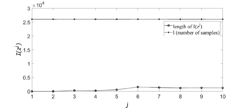
Figure 4: a9a: $|\mathcal{I}(z^{j})|$

Convergence of semismooth Newton’s method. To demonstrate the quadratic convergence of semismooth Newton’s method, we plot $\|F(w^{j})\|$ with respect to $j$ in the first loop of ALM for dataset leukemia. The result is demonstrated in Figure 5, where the quadratic convergence rate can be indeed observed.

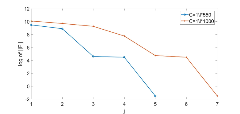
Figure 5: $\log\|F(w^{j})\|$ with C=$1/l*550$ and $1/l*1000$

Accuracy. Note that we are solving a practical problem, with predicting purpose. We are interested in the following question: as the iteration keeps on in ALM, what it happens to the accuracy? Below, we plot the accuracy vs outer iteration number $k$ in Figure 6. As we can see, the accuracy is reduced significantly during the first few iterations in ALM. However, little progress has been made after that. Consequently, we set the maximum number of outer iterations as $10$ in our test.

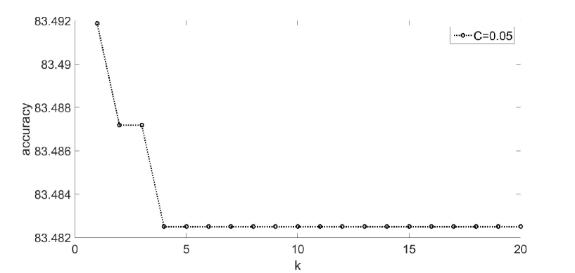
Figure 6: Accuracy during the update of ALM for a6a with $C=0.05$.

6.2 Performance with different parameters

It is noted that the choice of $C$ in L1-loss SVC (4) may have great influence on the performance of the algorithms. Consequently, in this part, we test our algorithms with different $C$s. To speed up the code, we try two choices. One is to generate starting point by solving subproblem (18) using alternating direction method of multipliers (ADMM). The other is to use a fixed starting point $w^{0}=ones(n,1)$. We report the results in Table 6.3 and 6.3. One can see that ALM-SNCG with fixed starting point has a better accuracy than that with ADMM as starting point. For cpu-time, using ADMM or not does not make much difference. For the choice of C, it seems that both values of $C=1/l*550,\ 1/l*1000$ give comparable accuracy and cpu-time. In our following test, we choose $C=1/l*550$ and use $w^{0}=ones(n,1)$ as our starting point.

6.3 Comparison with LIBLINEAR for SVC

As pointed out in [4], LIBLINEAR is the most popular solver. Consequently, in this part, we compare our algorithm with solvers in LIBLINEAR on dataset for SVC. We split each set to 80% training and 20% testing. Specifically, we compare with DCD which solves also model (4). Parameters in ALM are set as $\tau=1$, $\sigma_{0}=0.15$, $\sigma_{\max}=2$, $\theta=0.8$ and $\lambda_{0}=zeros(m,1)$. For semismooth Newton’s method, we choose $\rho=0.5$, $\delta=\max(1.0\times 10^{-2},\ 1.0\times 10^{-j})$. The results are reported in Table 6.3.

Comparison of Starting Points: C=1/l*550. I: $w^{0}=ones(n,1)$ as starting point; II: with ADMM as starting point dataset iter($k,it_{sn},it_{cg}$) times(s) accuracy($\%$) I II I II I II leukemia (1,5,11) (1,5,11) 0.015 0.097 100.000 100.000 a1a (1,11,77) (1,11,58) 0.036 0.033 84.819 84.787 a2a (1,11,80) (1,11,64) 0.029 0.031 84.818 84.769 a3a (1,9,70) (1,11,63) 0.024 0.028 84.717 84.717 a4a (1,10,73) (1,11,64) 0.028 0.027 84.737 84.773 a5a (1,10,78) (1,12,70) 0.022 0.034 84.780 84.761 a6a (1,9,67) (1,10,51) 0.022 0.021 84.587 84.587 a7a (1,11,89) (1,10,70) 0.019 0.018 84.604 84.573 a8a (1,9,72) (1,10,55) 0.019 0.020 84.031 83.965 a9a (1,11,84) (1,11,66) 0.031 0.030 84.677 84.692 w1a (1,14,99) (1,17,114) 0.057 0.072 99.958 99.958 w2a (1,12,84) (1,14,122) 0.062 0.061 99.968 99.957 w3a (1,17,141) (1,20,195) 0.093 0.148 99.955 99.955 w4a (1,13,95) (1,12,91) 0.059 0.067 99.953 99.953 w5a (2,22,168) (1,16,138) 0.105 0.087 99.950 99.950 w6a (1,17,170) (1,20,151) 0.068 0.065 99.923 99.923 w7a (1,14,100) (1,12,90) 0.031 0.033 99.900 99.900 w8a (1,14,114) (1,14,125) 0.060 0.062 99.950 99.950 breast-cancer (11,32,116) (11,32,108) 0.010 0.005 99.270 99.270 cod-rna (1,10,32) (1,9,31) 0.032 0.036 20.417 20.324 diabetes (11,35,114) (11,33,107) 0.006 0.004 75.974 75.974 fourclass (11,30,50) (11,28,47) 0.004 0.002 76.879 76.879 german.numer (11,44,305) (11,39,272) 0.020 0.016 78.500 78.500 heart (11,27,132) (11,28,141) 0.006 0.005 85.185 85.185 australian (11,37,232) (11,36,216) 0.009 0.007 86.232 86.232 ionosphere (11,33,189) (11,33,191) 0.006 0.010 98.592 98.592 covtype.binary (2,68,379) (1,46,377) 7.956 7.883 64.331 64.210 ijcnn1 (1,12,80) (1,9,36) 0.091 0.044 90.198 90.198 sonar (11,31,171) (11,31,171) 0.009 0.009 64.286 64.286 splice (11,42,230) (11,41,222) 0.021 0.023 80.500 80.500 svmguide1 (11,30,70) (11,30,79) 0.007 0.006 78.479 78.479 svmguide3 (11,34,134) (11,30,120) 0.013 0.013 0.000 0.000 phishing (1,14,101) (1,12,76) 0.047 0.043 92.492 92.583 madelon (11,51,445) (11,46,453) 0.743 0.864 52.250 52.250 mushrooms (2,34,393) (1,25,361) 0.202 0.220 100.000 100.000 duke breast-cancer (1,7,14) (1,6,13) 0.022 0.132 100.000 100.000 gisette (4,187,1174) (3,117,1570) 20.870 23.454 97.583 97.500 news20.binary (11,29,61) (11,29,61) 4.463 4.389 11.275 11.275 rcv1-train.binary (11,61,142) (11,36,111) 0.537 0.479 94.394 94.394 real-sim (1,32,43) (1,12,33) 0.436 0.406 80.729 80.556 liver-disorders (11,22,44) (11,22,42) 0.005 0.002 55.172 55.172 colon-cancer (1,7,16) (1,7,15) 0.009 0.014 69.231 69.231 skin-nonskin (1,8,20) (1,9,18) 0.157 0.170 90.429 90.413

Comparison of Starting Points: C=1/l*1000 dataset iter($k,it_{sn},it_{cg}$) time(s) accuracy($\%$) I II I II I II leukemia (1,7,13) (1,6,12) 0.027 0.121 100.000 100.000 a1a (8,36,284) (8,31,227) 0.099 0.079 84.868 84.868 a2a (10,33,302) (10,40,280) 0.107 0.096 84.835 84.835 a3a (11,41,346) (11,39,308) 0.098 0.095 84.717 84.717 a4a (11,35,304) (11,43,305) 0.100 0.107 84.791 84.791 a5a (10,33,280) (10,35,263) 0.080 0.079 84.665 84.665 a6a (10,33,294) (11,42,291) 0.080 0.093 84.657 84.657 a7a (11,36,302) (10,37,275) 0.065 0.066 84.604 84.604 a8a (11,42,320) (11,37,295) 0.075 0.077 84.141 84.141 a9a (9,38,322) (9,38,270) 0.109 0.096 84.738 84.738 w1a (1,18,157) (2,18,135) 0.075 0.072 99.905 99.926 w2a (1,13,97) (1,16,157) 0.054 0.080 99.924 99.924 w3a (1,15,142) (1,17,123) 0.059 0.061 99.944 99.933 w4a (1,15,132) (1,20,156) 0.082 0.108 99.929 99.929 w5a (1,14,102) (1,13,89) 0.059 0.048 99.887 99.900 w6a (1,19,148) (1,15,109) 0.058 0.049 99.893 99.877 w7a (1,17,131) (5,27,219) 0.047 0.066 99.900 99.920 w8a (1,19,171) (1,21,157) 0.104 0.097 99.920 99.920 breast-cancer (11,33,130) (11,32,124) 0.004 0.005 99.270 99.270 cod-rna (1,17,44) (1,11,35) 0.068 0.045 21.542 21.492 diabetes (11,33,102) (11,31,96) 0.005 0.004 74.675 74.675 fourclass (11,30,49) (11,28,46) 0.002 0.005 76.879 76.879 german.numer (11,42,305) (11,39,304) 0.017 0.019 77.500 77.500 heart (11,24,118) (11,25,127) 0.004 0.003 88.889 88.889 australian (11,34,195) (11,32,171) 0.006 0.006 86.957 86.957 ionosphere (11,30,158) (11,29,151) 0.006 0.007 97.183 97.183 covtype.binary (3,120,489) (3,107,505) 14.295 13.708 64.738 64.769 ijcnn1 (11,34,221) (11,33,205) 0.267 0.208 90.378 90.378 sonar (11,30,172) (11,30,172) 0.022 0.057 64.286 64.286 splice (11,41,212) (11,39,198) 0.031 0.028 81.500 81.500 svmguide1 (11,32,91) (11,32,96) 0.011 0.008 86.408 86.408 svmguide3 (11,32,149) (11,31,152) 0.023 0.014 0.000 0.000 phishing (10,47,363) (10,41,305) 0.205 0.117 92.492 92.492 madelon (11,67,478) (11,44,420) 1.148 1.068 50.000 50.000 mushrooms (1,31,244) (1,26,258) 0.125 0.171 100.000 100.000 duke breast-cancer (1,8,15) (1,9,16) 0.024 0.103 100.000 100.000 gisette (6,266,1270) (5,235,1159) 26.389 20.597 97.250 97.500 news20.binary (11,32,78) (11,32,78) 5.769 5.760 49.850 49.850 rcv1-train.binary (10,111,194) (11,35,125) 1.302 0.613 95.357 95.357 real-sim (11,72,119) (1,16,49) 1.050 1.007 74.582 74.063 liver-disorders (11,22,44) (11,22,42) 0.011 0.005 55.172 55.172 colon-cancer (1,6,14) (1,6,18) 0.007 0.011 69.231 69.231 skin-nonskin (1,11,27) (1,13,24) 0.189 0.218 90.235 90.231

The comparison results for L1-loss SVC. dataset time(s)(DCD$|$ALM-SNCG) accuracy($\%$)(DCD$|$ALM-SNCG) leukemia 0.017 $|$ 0.015 100.000 $|$ 100.000 a1a 0.059 $|$ 0.036 84.722 $|$ 84.819 a2a 0.049 $|$ 0.029 84.752 $|$ 84.818 a3a 0.044 $|$ 0.024 84.700 $|$ 84.717 a4a 0.042 $|$ 0.028 84.683 $|$ 84.737 a5a 0.040 $|$ 0.022 84.627 $|$ 84.780 a6a 0.033 $|$ 0.022 84.516 $|$ 84.587 a7a 0.026 $|$ 0.019 84.482 $|$ 84.604 a8a 0.033 $|$ 0.019 84.119 $|$ 84.031 a9a 0.068 $|$ 0.031 84.708 $|$ 84.677 w1a 0.088 $|$ 0.057 99.662 $|$ 99.958 w2a 0.071 $|$ 0.062 99.676 $|$ 99.968 w3a 0.103 $|$ 0.093 99.699 $|$ 99.955 w4a 0.077 $|$ 0.059 99.705 $|$ 99.953 w5a 0.121 $|$ 0.105 99.737 $|$ 99.950 w6a 0.047 $|$ 0.068 99.754 $|$ 99.923 w7a 0.039 $|$ 0.031 99.721 $|$ 99.900 w8a 0.094 $|$ 0.060 99.668 $|$ 99.950 breast-cancer 0.001 $|$ 0.010 100.000 $|$ 99.270 cod-rna 0.066 $|$ 0.032 19.879 $|$ 20.417 diabetes 0.001 $|$ 0.006 74.675 $|$ 75.974 fourclass 0.001 $|$ 0.004 68.786 $|$ 76.879 german.numer 0.004 $|$ 0.020 78.000 $|$ 78.500 heart 0.002 $|$ 0.006 81.481 $|$ 85.185 australian 0.001 $|$ 0.009 86.232 $|$ 86.232 ionosphere 0.006 $|$ 0.006 98.592 $|$ 98.592 covtype.binary 12.086 $|$ 7.956 64.094 $|$ 64.331 ijcnn1 0.125 $|$ 0.091 90.198 $|$ 90.198 sonar 0.006 $|$ 0.009 64.286 $|$ 64.286 splice 0.016 $|$ 0.021 69.500 $|$ 80.500 svmguide1 0.001 $|$ 0.007 53.560 $|$ 78.479 svmguide3 0.002 $|$ 0.013 0.000 $|$ 0.000 phishing 0.081 $|$ 0.047 92.763 $|$ 92.492 madelon 0.181 $|$ 0.743 52.500 $|$ 52.250 mushrooms 0.131 $|$ 0.202 100.000 $|$ 100.000 duke breast-cancer 0.034 $|$ 0.022 100.000 $|$ 100.000 gisette 3.796 $|$ 19.270 97.333 $|$ 97.583 news20.binary 0.642 $|$ 4.463 27.775 $|$ 11.275 rcv1-train.binary 0.123 $|$ 0.537 94.443 $|$ 94.394 real-sim 0.353 $|$ 0.436 72.383 $|$ 80.729 liver-disorders 0.000 $|$ 0.005 41.379 $|$ 55.172 colon-cancer 0.006 $|$ 0.009 69.231 $|$ 69.231 skin-nonskin 0.171 $|$ 0.157 88.236 $|$ 90.429

We can get the following observations from the results.

• Both of the two algorithms can obtain high accuracy. We marked the winners of cpu-time and accuracy in bold. The accuracy of more than 80% of datasets is over 72%, and some datasets’s accuracy is more than 90%. In comparison with DCD for the 43 classification datasets, ALM-SNCG has equal or higher accuracy for 36 datasets. In particular, for dataset fourclass, splice, svmguide1, real-sim, and liver-disorders, the accuracy of ALM-SNCG has increased by nearly 10% or even more than 10% (marked in red).

• In terms of cpu-time, ALM-SNCG is competitive with DCD. For example, for the dataset covtype.binary, ALM-SNCG saves cpu-time by almost 50%. For all the 43 datasets, ALM-SNCG is faster than DCD for 24 datasets.

6.4 Comparison with LIBLINEAR for SVR

In this part, we compare our algorithm with DCD [12] in LIBLINEAR on dataset for SVR (5). We split each dataset to 60% training and 40% testing. We choose C = 1/n*5. Parameters in Algorithm 3.4 are set as $\sigma_{0}=0.1$ and other parameters are set as the same in SVC. The results are reported in Table 6.4, from which we have the following observations.

• In comparison with DCD for the 13 regression datasets, ALM-SNCG has equal or higher accuracy for all the 13 datasets.

• In terms of cpu-time, ALM-SNCG is competitive with DCD. For example, for the dataset E2006-train, ALM-SNCG saves cpu-time by more than 50%. For all the 13 datasets, ALM-SNCG has equal or shorter cpu-time for 10 datasets.

The comparison results for SVR. dataset time(s)(DCD$|$ALM-SNCG) mse(DCD$|$ALM-SNCG) abalone 0.002 $|$ 0.002 27.47 $|$ 12.85 bodyfat 0.001 $|$ 0.001 0.02 $|$ 0.01 cadata 0.014 $|$ 0.008 0.17 $|$ 0.15 cpusmall 0.004 $|$ 0.001 2253.55 $|$ 1862.67 E2006-train 1.517 $|$ 0.733 0.31 $|$ 0.29 E2006-test 0.316 $|$ 0.349 0.23 $|$ 0.21 eunite2001 0.001 $|$ 0.001 539999.28 $|$ 532688.85 housing 0.001 $|$ 0.001 134.79 $|$ 93.77 mg 0.000 $|$ 0.001 0.42 $|$ 0.02 mpg 0.000 $|$ 0.000 862.10 $|$ 606.14 pyrim 0.000 $|$ 0.001 0.02 $|$ 0.01 space-ga 0.001 $|$ 0.001 0.26 $|$ 0.03 triazines 0.002 $|$ 0.002 0.03 $|$ 0.03

7 Conclusions

In this paper, we proposed a semismooth Newton-CG based on augmented Lagrangian method for solving the L1-loss SVC and $\epsilon$-L1-loss SVC. The proposed algorithm enjoyed the traditional convergence result while keeping the fast quadratic convergence and low computational complexity in semismooth Newton algorithm as a subsolver. Extensive numerical results on datasets in LIBLINEAR demonstrated the superior performance of the proposed algorithm over the LIBLINEAR in terms of both accuracy and speed.

Acknowledgements.
We would like to thank the three anonymous reviewers for there valuable comments which helped improve the paper significantly. We would also like to thank Prof. Chao Ding from Chinese Academy of Sciences for providing the important reference of Prof. Jie Sun’s PhD thesis. We would also like to thank Dr. Xudong Li from Fudan University for helpful discussions.

Notes on contributors.
Yinqiao Yan received his Bachelor of science in statistics degree from Beijing Institute of Technology, China, in 2019. He is pursuing his PhD degree in Institute of Statistics and Big Data, Renmin University of China, China.

Qingna Li received her Bachelor’s degree in information and computing science and Doctor’s degree in computational mathematics from Hunan University, China, in 2005 and 2010 respectively. Currently, she is an associate professor in School of Mathematics and Statistics, Beijing Institute of Technology. Her research interests include continuous optimization and its applications.

Appendix. The calculation of $\hbox{Prox}_{p}^{M}(z)$

Note that

$$\min_{s}\frac{1}{2M}\|z-s\|^{2}+C\sum_{i=1}^{m}\max(0,s_{i})$$

$$\Longleftrightarrow \min_{s}\sum_{i=1}^{m}(\frac{1}{2M}(z_{i}-s_{i})^{2}+C\max(0,s_{i}))$$

$$\Longleftrightarrow \min_{s_{i}}\frac{1}{2M}(z_{i}-s_{i})^{2}+C\max(0,s_{i}),\ i=1,\dots,m.$$

For each $i$, consider solving the following problem

$$\min_{s_{i}}\frac{1}{2M}(z_{i}-s_{i})^{2}+C\max(0,s_{i}).$$

This is a problem of minimizing a piecewise quadratic function. The objective function of this problem takes the following form

$$\left\{\begin{aligned} &\frac{1}{2M}(z_{i}-s_{i})^{2},\ &s_{i}\leq 0,\\ &\frac{1}{2M}s_{i}^{2}+(C-\frac{1}{M}z_{i})s_{i}+\frac{1}{2M}z_{i}^{2},\ &s_{i}>0.\end{aligned}\right.$$

One can see that the solution is

$$s_{i}^{*}=\left\{\begin{array}[]{ll}z_{i}-CM,&z_{i}>CM,\\ z_{i},&z_{i}<0,\\ 0,&0\leq z_{i}\leq CM.\end{array}\right.$$

Therefore, we get that

$$(\hbox{Prox}_{p}^{M}(z))_{i}=\left\{\begin{array}[]{ll}z_{i}-CM,&z_{i}>CM,\\ z_{i},&z_{i}<0,\\ 0,&0\leq z_{i}\leq CM.\end{array}\right.$$

References

- [1] D. Basak, S. Pal and D. Patranabis, Support vector regression, Neural Information Processing - Letters and Reviews, 11(10) (2007), pp. 203-224.
- [2] B.E. Boser, I.M. Guyon, and V.N. Vapnik, A training algorithm for optimal margin classifiers, in COLT’92: Proceedings of the 5th annual ACM Workshop on Computational Learning Theory, Pittsburgh, PA, 27-29 July 1992, pp. 144-152.
- [3] O. Chapelle, Training a support vector machine in the primal, Neural Comput., 19(5) (2007), pp. 1155-1178.
- [4] V.K. Chauhan, K. Dahiya, and A. Sharma, Problem formulations and solvers in linear SVM: a review, Artif Intell Rev, 2019, pp. 803-855. https://doi.org/10.1007/s10462-018-9614-6.
- [5] F.H. Clarke, Optimization and Nonsmooth Analysis, John Wiley Sons, New York, 1933
- [6] M. Collins, A. Globerson, T. Koo, X. Carreras, and P. Bartlett, Exponentiated gradient algorithms for conditional random elds and max-margin Markov networks, J. Mach. Learn. Res., 9 (2008), pp. 1775-1822.
- [7] C. Cortes and V.N. Vapnik, Support-vector networks, Mach. Learn., 20(3) (1995), pp. 273-297.
- [8] H. Drucker, C.J.C. Burges, L. Kaufman, A.J. Smola, and V.N. Vapnik, Support vector regression machines, Adv. Neural. Inf. Process. Syst., 28 (1997), pp. 779-784.
- [9] R. Fan, K. Chang, C. Hsieh, X. Wang, C. Lin, (2008) LIBLINEAR: a library for large linear classification, JMLR, 9 (2008), pp. 1871-1874.
- [10] W. Gu, W.P. Chen, and C.H. Ko, Two smooth support vector machines for -insensitive regression. Comput. Optim. Appl., 70 (2018), pp. 1-29.
- [11] M.R. Hestenes and E. Stiefel, Methods of conjugate gradients for solving linear systems, J. Res. Natl. Bur. Stand., 49 (1952), pp. 409-436
- [12] C.H. Ho and C.-J. Lin, Large-scale linear support vector regression, J. Mach. Learn. Res., 13(Nov) (2012), pp. 3323-3348.
- [13] C.J. Hsieh, K.W. Chang, C.-J. Lin, S.S. Keerthi, and S. Sundararajan, A dual coordinate descent method for large-scale linear SVM, in Proceedings of the 25th international conference on Machine learning, Helsinki, Finland, pp. 408-415.
- [14] N. Ito, A. Takeda, and K.-C. Toh, A unified formulation and fast accelerated proximal gradient method for classification, JMLR, 18(1) (2017), pp. 510-558.
- [15] T. Joachims, Making large-scale support vector machine learning practical, in Advances in Kernel Methods - Support Vector Learning, B. Scholkopf, C. Burges, and A. Smola, eds., MIT Press, Cambridge, MA, 1999, pp. 169-184.
- [16] T. Joachims, Training linear SVMs in linear time, in Proceedings of the 12th ACM SIGKDD international conference on Knowledge discovery and data mining, ACM, Philadelphia, PA, USA, 2006, pp. 217-226.
- [17] C. Kanzow, Inexact semismooth Newton methods for large-scale complementarity problems, Optimization Methods and Software, 19(3-4) (2004), pp. 309-325.
- [18] J. Kivinen, A.J. Smola, and R.C. Williamson, Online learning with kernels, IEEE Trans. Signal Process. 52(8) (2002), pp. 2165-2176.
- [19] Q.N. Li and H.-D. Qi, A sequential semismooth Newton method for the nearest low-rank correlation matrix problem, SIAM J. Optim., 21(4) (2011), pp. 1641-1666.
- [20] X.D. Li, D.F. Sun, and K.-C. Toh, A highly efficient semismooth Newton augmented Lagrangian method for solving Lasso problems, SIAM J. Optim., 28(1) (2018), pp. 433-458.
- [21] Y.-J. Liu, D.F. Sun, K.-C. Toh, An implementable proximal point algorithmic framework for nuclear norm minimization, Math. Program., 133(1-2) (2012), pp. 399-436. https://doi.org/10.1007/s10107-010-0437-8.
- [22] Z.Y. Luo, D.F. Sun, and K.-C. Toh, Solving the OSCAR and SLOPE models using a semismooth Newton-based augmented Lagrangian method, preprint(2018). Available at arXiv, math. OC/1803.10740.
- [23] R. Mifflin, Semismooth and semiconvex functions in constrained optimization, SIAM J. Control Optim., 15(6) (1977), pp. 959-972.
- [24] J.J. Moreau, Proximite dt dualite dans un espace hilbertien, Bulletin de la Societe Mathematique de France, 93 (1965), pp. 273-299.
- [25] F. Nie, Y. Huang, X. Wang, and H. Huang, New primal SVM solver with linear computational cost for big data classifications, in Proceedings of the 31st International Conference on Machine Learning, Beijing, China, Vol. 32 (2014), pp. II-505-II-513.
- [26] D. Niu, C. Wang, P. Tang, Q. Wang, and E. Song, A sparse semismooth Newton based augmented Lagrangian method for large-scale support vector machines, 2019. Available at arXiv, math. OC/1910.01312.
- [27] J.C. Platt, Fast training of support vector machines using sequential minimal optimization, in Advances in Kernel Methods - Support Vector Learning, B. Scholkopf, C. Burges, and A. Smola, eds., MIT Press, Cambridge, MA, 1998, pp. 185-208.
- [28] H.-D. Qi, A semismooth Newton method for the nearest Euclidean distance matrix problem, SIAM J. Matrix Anal. Appl., 34(1) (2013), pp. 67-93.
- [29] H.-D. Qi and D.F. Sun, A quadratically convergent Newton method for computing the nearest correlation matrix, SIAM J. Matrix Anal. Appl., 28(2) (2006), pp. 360-385.
- [30] H.-D. Qi and X.M. Yuan, Computing the nearest Euclidean distance matrix with low embedding dimensions, Math. Program., 147(1-2) (2014), pp. 351-389.
- [31] L. Qi and J. Sun, A nonsmooth version of Newton’s method, Math. Program., 58(1-3) (1993), pp. 353-367.
- [32] R.T. Rockafellar, Augmented Lagrangians and applications of the proximal point algorithm in convex programming, Math. Oper. Res., 1(2) (1976), pp. 97-116.
- [33] R.T. Rockafellar, Monotone operators and the proximal point algorithm, SIAM J. Control Optim., 14(5) (1976), pp. 877-898.
- [34] S. Shalev-Shwartz, Y. Singer, and N. Srebro, Pegasos: primal estimated sub-gradient solver for SVM, International Conference on Machine Learning, Oregon State University, Corvallis, USA, 2007.
- [35] A.J. Smola, Regression estimation with support vector learning machines, Master thesis, Technische Universitt Mnchen, 1996.
- [36] A.J. Smola, S.V.N. Vishwanathan, and Q. Le, Bundle methods for machine learning, in J.C. Platt, D. Koller, Y. Singer, and S. Roweis, eds., Advances in Neural Information Processing Systems 20, MIT Press, Cambridge, MA, 2008, pp. 1377-1384.
- [37] D. F. Sun and J. Sun, Semismooth matrix-valued functions, Math. Oper. Res., 27 (2002), pp. 150-169.
- [38] D.F. Sun, K.-C. Toh, and L.Q. Yang, An efficient inexact ABCD method for least squares semidefinite programming, SIAM J. Optim., 26(2) (2016), pp. 1072-1100.
- [39] D.F. Sun, K.-C. Toh, and Y.C. Yuan, Convex clustering: model, theoretical guarantee and efficient algorithm, preprint (2018). Available at arXiv, cs. LG/1810.02677.
- [40] D.F. Sun, K.-C. Toh, Y.C. Yuan, and X.Y. Zhao, SDPNAL+: A Matlab software for semidefinite programming with bound constraints (version 1.0), Optimization Methods and Software, 2019, pp. 1-29. Available at arXiv, math. OC/1710.10604.
- [41] J. Sun, On monotropic piecewise quadratic programming, PhD thesis, Department of Mathematics, University of Washington, 1986.
- [42] M. Tak, A. Bijral, P. Richtrik, and N. Srebro, Mini-batch primal and dual methods for SVMs, in Proceedings of the 30th International Conference on Machine Learning, Atlanta, USA, 2013.
- [43] L.Q. Yang, D.F. Sun, and K.-C. Toh, SDPNAL+: A majorized semismooth Newton-CG augmented Lagrangian method for semidefinite programming with nonnegative constraints, Math. Program. Comput., 7(3) (2015), pp. 331-366.
- [44] J. Yin and Q.N. Li, A semismooth Newton method for support vector classification and regression, Comput. Optim. Appl., 2019, DOI: 10.1007/s10589-019-00075-z.
- [45] K. Yosida, Functional Analysis, Springer Verlag, Berlin, 1964.
- [46] F.Z. Zhai and Q.N. Li, A Euclidean distance matrix model for protein molecular conformation, J. Global Optim., 2019, DOI: 10.1007/s10898-019-00771-4.
- [47] T. Zhang, Solving large scale linear prediction problems using stochastic gradient descent algorithms, in Proceedings of the 21th International Conference on Machine Learning, Banff, Alberta, Canada, 2004.
- [48] X.Y. Zhao, A semismooth Newton-CG augmented Lagrangian method for large scale linear and convex quadratic SDPS. Ph.D. diss., National University of Singapore, 2009.
- [49] X.Y. Zhao, D.F. Sun, and K.-C. Toh, A Newton-CG augmented Lagrangian method for semidefinite programming, SIAM J. Optim., 20 (2010), pp. 1737-1765.
- [50] P. Zhong and M. Fukushima, Regularized nonsmooth Newton method for multi-class support vector machines, Optimization Methods and Software, 22(1) (2007), pp. 225-236