Cross-Batch Memory for Embedding Learning

Abstract

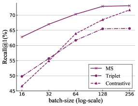
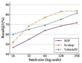
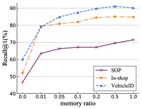
Figure 1: R@1 results with GoogleNet. Left: R@1 on SOP $vs.$ mini-batch size with contrastive, triplet and MS approaches. Middle: R@1 $vs.$ mini-batch size by varying datasets. Right R@1 $vs.$ memory ratio at mini-batch size 16 with contrastive loss.

Mining informative negative instances are of central importance to deep metric learning (DML), however this task is intrinsically limited by mini-batch training, where only a mini-batch of instances is accessible at each iteration. In this paper, we identify a “slow drift” phenomena by observing that the embedding features drift exceptionally slow even as the model parameters are updating throughout the training process. This suggests that the features of instances computed at preceding iterations can be used to considerably approximate their features extracted by the current model. We propose a cross-batch memory (XBM) mechanism that memorizes the embeddings of past iterations, allowing the model to collect sufficient hard negative pairs across multiple mini-batches - even over the whole dataset. Our XBM can be directly integrated into a general pair-based DML framework, where the XBM augmented DML can boost performance considerably. In particular, without bells and whistles, a simple contrastive loss with our XBM can have large R@1 improvements of 12%-22.5% on three large-scale image retrieval datasets, surpassing the most sophisticated state-of-the-art methods [37, 26, 2], by a large margin. Our XBM is conceptually simple, easy to implement - using several lines of codes, and is memory efficient - with a negligible 0.2 GB extra GPU memory. Code is available at: https://github.com/MalongTech/research-xbm.

1 Introduction

Deep metric learning (DML) aims to learn an embedding space where instances from the same class are encouraged to be closer than those from different classes. As a fundamental problem in computer vision, DML has been applied to various tasks, including image retrieval [39, 12, 7], face recognition [38], zero-shot learning [47, 1, 16], visual tracking [17, 34] and person re-identification [44, 13].

A family of DML approaches are known as pair-based, whose objectives can be defined in terms of pair-wise similarities within a mini-batch, such as contrastive loss [3], triplet loss [29], lifted-structure loss[22], n-pairs loss [30], multi-similarity (MS) loss [37] and etc. Moreover, most existing pair-based DML methods can be unified as weighting schemes under a General Pair Weighting (GPW) framework [37]. The performance of pair-based methods heavily rely on their capability of mining informative negative pairs. To collect sufficient informative negative pairs from each mini-batch, many efforts have been devoted to improving the sampling schemes, which can be categorized into two main directions: (1) sampling informative mini-batches based on global data distribution [32, 6, 28, 32, 9]; (2) weighting informative pairs within each individual mini-batch [22, 30, 37, 35, 40].

Various sophisticated sampling schemes have been developed, but the hard mining ability is inherently limited by the size of a mini-batch, which the number of possible training pairs depends on. Therefore, to improve the sampling scheme, it is straightforward to enlarge the mini-batch, which can boost the performance of pair-based DML methods immediately. We demonstrate by experiments that the performance of pair-based approaches, such as contrastive loss [3] and recent MS loss [37], can be improved strikingly when the mini-batch grows larger on large-scale datasets (Figure 1, left and middle). It is not surprising because the number of negative pairs grows quadratically w.r.t. the mini-batch size. However, simply enlarging a mini-batch is not an ideal solution to solve the hard mining problem due to two limitations: (1) the mini-batch size is limited by the GPU memory and computational cost; (2) a large mini-batch (e.g. 1800 used in [29]) often requires cross-device synchronization, which is a challenging engineering task. A naive solution to collect abundant informative pairs is to compute the features of instances in the whole training set at each training iteration, and then search for hard negative pairs from the whole dataset. Obviously, this solution is extremely time consuming, especially for a large-scale dataset, but it inspired us to break the limit of mining hard negatives within a single mini-batch.

In this paper, we identify an interesting “slow drift” phenomena that the embedding of an instance actually drifts at a relatively slow rate throughout the training process. It suggests that the deep features of a mini-batch computed at past iterations can considerably approximate to those extracted by current model. Based on the “slow drift” phenomena, we propose a cross-batch memory (XBM) module to record and update the deep features of recent mini-batches, allowing for mining informative examples across multiple mini-batches. Our XBM can provide plentiful hard negative pairs by directly connecting each anchor in the current mini-batch with the embeddings from recent mini-batches.

Our XBM is conceptually simple, easy to implement and memory efficient. The memory module can be updated using a simple enqueue-dequeue mechanism by leveraging the computation-free features computed at the past iterations, with only about a negligible 0.2 GB of extra GPU memory utilized. More importantly, our XBM can be directly integrated into most existing pair-based methods with just several lines of codes, and can boost performance considerably. We evaluate our XBM with various conventional pair-based DML techniques on three widely used large-scale image retrieval datasets: Stanford Online Products (SOP) [22], In-shop Clothes Retrieval (In-shop) [20], and PKU VehicleID (VehicleID) [19]. In Figure 1 (middle and right), our approach demonstrates excellent robustness and brings consistent performance improvements across all settings; under the same configurations, our XBM obtains extraordinary R@1 improvements on all three datasets compared with the corresponding pair-based methods (e.g. over 20% for contrastive loss). Furthermore, with our XBM, a simple contrastive loss can easily outperform the most state-of-the-art sophisticated methods, such as [37, 26, 2], by a large margin.

In parallel to our work, He et al. [10] built a dynamic dictionary as a queue of preceding mini-batches to provide a rich set of negative samples for unsupervised learning (with a contrastive loss). However, unlike [10] which uses a specific encoding network to compute the features of current mini-batch, our features are computed more efficiently by taking them directly from the forward of the current model with no additional computational cost. More importantly, to solve the problem of feature drift, He et al. designed a momentum update that slowly progresses the key encoder to ensure the consistency between different iterations, while we identify the “slow drift” phenomena which suggests that the features can become stable by themselves when the early phase of training finishes.

2 Related Work

Pair-based DML. Pair-based DML methods can be optimized by computing the pair-wise similarities between instances in the embedding space [8, 22, 29, 35, 30, 37]. Contrastive loss [8] is one of the classic pair-based DML methods, which learns a discriminative metric via Siamese networks. It encourages the deep features of positive pairs to be closer to each other, and those of negative pairs to be farther than a fixed threshold. Triplet loss [29] requires the similarity of a positive pair to be higher than that of a negative pair (with the same anchor) by a given margin.

Inspired by contrastive loss and triplet loss, a number of pair-based DML algorithms have been developed, which attempted to weight all pairs in a mini-batch, such as up-weighting informative pairs (e.g. N-pair loss [30], Multi-Similarity (MS) loss [37]) through a log-exp formulation, or sampling negative pairs uniformly w.r.t. pair-wise distance [40]. Generally, pair-based methods can be cast into a unified weighting formulation through General Pair Weighting (GPW) framework [37].

However, most deep models are trained with SGD where only a mini-batch of samples are accessible at each iteration, and the size of a mini-batch can be relatively small compared to the whole dataset, especially for a large-scale dataset. Moreover, a large fraction of the pairs is less informative as the model learns to embed most trivial pairs correctly. Thus the conventional pair-based DML techniques suffer from lacks of hard negative pairs, which are critical to promote model training.

To alleviate the aforementioned problems, a number of approaches have been developed to collect more potential information contained in a mini-batch, such as building a class-level hierarchical tree [6], updating class-level signatures to select hard negative instances [32], or obtaining samples from an individual cluster [28]. Unlike these approaches which aim to enrich the information in a mini-batch, our XBM are designed to directly mine hard negative examples across multiple mini-batches.

Proxy-based DML. There is another branch of DML methods aiming to learn the embeddings by comparing each sample with proxies, including proxy NCA [21], NormSoftmax [46] and SoftTriple [25]. In fact, our XBM module can be regarded as the proxies to some extent. However, there are two main differences between the proxy-based methods and our XBM module: (1) proxies are often optimized along with the model weights, while the embeddings of our memory are directly taken from the past mini-batches; (2) proxies are used to represent the class-level information, whereas the embedding of our memory computes the information for each individual instance. Both proxy-based methods and our XBM augmented pair-based methods are able to capture the global distribution of data over the whole dataset during training.

Feature Memory Module. Non-parametric memory module for embedding learning has shown power in various computer visual tasks [36, 43, 41, 42, 48, 18]. For examples, the external memory can be used to address the unaffordable computational demand of conventional NCA [41] in large-scale recognition, and encourage instance-invariance in domain adaptation [48, 42]. But only the positive pairs are optimized, while the negatives are ignored in [41]. Our XBM is able to to provide a rich set of negative examples for the pair-based DML methods, which is more generalized and can make full use of the past embeddings. The key distinction is that existing memory modules only store the embeddings of current mini-batch [36], or maintain the whole dataset [41, 48] with a moving average update, while our XBM is maintained as a dynamic queue of mini-batches, which is more flexible and applicable in extremely large-scale datasets.

3 Cross-Batch Memory Embedding Networks

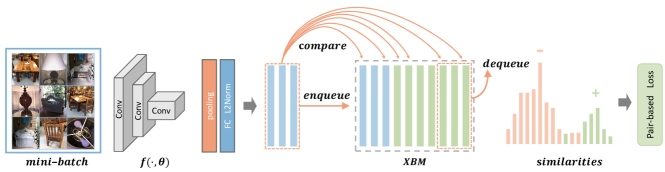
Figure 2: Cross-Batch Memory (XBM) trains an embedding network by comparing each anchor with a memory bank using a pair-based loss. The memory bank is maintained as a queue with the current mini-batch enqueued and the oldest mini-batch dequeued. Our XBM enables a large amount of valid negatives for each anchor to benefit the model training with many pair-based methods.

In this section, we first analyze the limitation of existing pair-based DML methods. Then we introduce the “slow drift” phenomena, which provides the underlying evidence that supports our cross-batch mining approach. Finally, we describe our XBM module and integrate it into existing pair-based DML methods.

3.1 Delving into Pair-based DML

Let ${\mathbb{X}}=\{{\bm{x}}_{1},{\bm{x}}_{2},\dots,{\bm{x}}_{N}\}$ denotes a set of training instances, and $y_{i}$ is the corresponding label of ${\bm{x}}_{i}$. An embedding function, $f(\cdot;{\bm{\theta}})$, projects a data point ${\bm{x}}_{i}$ onto a $D$-dimensional unit hyper-sphere, ${\bm{v}}_{i}=f({\bm{x}}_{i};{\bm{\theta}})$. We measure the similarity between two instances of a pair in the embedding space. During training, we denote an affinity matrix of all pairs within the current mini-batch as ${\bm{S}}$, whose $(i,j)$ element is the cosine similarity between the embeddings of the $i$-th sample and the $j$-th sample: ${\bm{v}}_{i}^{T}{\bm{v}}_{j}$.

To facilitate further analysis, we delve into the pair-based DML methods by using the GPW framework described in [37]. With GPW, a pair-based function can be formulated in a unified pair-weighting form:

$$\small\mathcal{L}=\frac{1}{m}\sum_{i=1}^{m}\left[\sum_{y_{j}\neq y_{i}}^{m}w_{ij}{\bm{S}}_{ij}-\sum_{y_{j}=y_{i}}^{m}w_{ij}{\bm{S}}_{ij}\right],$$ (1)

where $m$ is the mini-batch size, and $w_{ij}$ is the weight assigned to ${\bm{S}}_{ij}$. Eq. 1 shows that any pair-based method can be considered as a weighting scheme focusing on informative pairs. Here we list the weighting schemes of contrastive loss, triplet loss and MS loss.

• Contrastive loss. For each negative pair, $w_{ij}=1$ if ${\bm{S}}_{ij}>\lambda$, otherwise $w_{ij}=0$. The weights of all positive pairs are set to 1.

• Triplet loss. For each negative pair, $w_{ij}=|\mathcal{P}_{ij}|$, where $\mathcal{P}_{ij}$ is the valid positive set sharing the anchor. Formally, $\mathcal{P}_{ij}=\{{\bm{x}}_{i,k}|y_{k}=y_{i},\ \text{and}\ {\bm{S}}_{ik}<{\bm{S}}_{ij}+\eta\}$ and $\eta$ is a predefined margin in triplet loss. Similarly, we can obtain the triplet weight for a positive pair.

• MS loss. Unlike contrastive loss and triplet loss which only assigns a weight with integer value, MS loss [37] is able to weight the pairs more properly by jointly considering multiple similarities. The MS weight for a negative pair is computed as:

  $$\small w_{ij}=\frac{e^{\beta\left({\bm{S}}_{ij}-\lambda\right)}}{1+\sum\limits_{k\in\mathcal{N}_{i}}e^{\beta\left({\bm{S}}_{ik}-\lambda\right)}},$$

  where $\beta$ and $\lambda$ are hyper-parameters, and $\mathcal{N}_{i}$ is the valid negative set for the anchor ${\bm{x}}_{i}$. The MS weight for a positive pair can be computed similarly.

In fact, the main path of developing pair-based DML is to design a better weighting mechanism for pairs within a mini-batch. Generally, with a small mini-batch (e.g. 16 or 32), the sophisticated weighting schemes can perform much better (Figure 1, left). However, beyond the weighting scheme, the mini-batch size is also of great importance to DML. Figure 1 (left and middle) shows the R@1s of various pair-based methods are increased considerably by using a larger mini-batch on large-scale datasets. Intuitively, the number of negative pairs increase quadratically when the mini-batch size grows, which naturally provides more informative pairs. Instead of developing another sophisticated but highly complicated algorithm to weight the informative pairs, our intuition is to simply collect sufficient informative negative pairs, where a simple weighting scheme, such as contrastive loss, can easily outperform the stage-of-the-art weighting approaches. This provides a new path that is straightforward yet more efficient to solve the hard mining problem in DML.

Naively, a straightforward solution to collect more informative negative pairs is to increase the mini-batch size. However, training deep networks with a large mini-batch is limited by GPU memory, and often requires massive data flow communication between multiple GPUs. To this end, we attempt to achieve the same goal by introducing an alternative approach using very low GPU memory and minimum computation burden. We propose a XBM module that allows the model to collect informative pairs over multiple past mini-batches, based on the “slow drift” phenomena as described below.

3.2 Slow Drift Phenomena

The embeddings of past mini-batches are usually considered out-of-date because the model parameters are changing throughout the training process [10, 32, 25]. Such out-of-date features are always discarded, but we learn that they can be an important resource, while being computation-free, by identifying the “slow drift” phenomena. We study the drifting speed of embeddings by measuring the difference of features for the same instance computed at different training iterations. Formally, the feature drift of an input ${\bm{x}}$ at $t$-th iteration with step $\Delta t$ is defined as:

$$\begin{split}D(x,t;\Delta t)&\mathrel{\vbox{\hbox{\scriptsize.}\hbox{\scriptsize.}}}=||f({\bm{x}};{\bm{\theta}}^{t})-f({\bm{x}};{\bm{\theta}}^{t-\Delta t})||_{2}^{2}\\ \end{split}$$ (2)

We train GoogleNet [33] from scratch with a contrastive loss, and compute the average feature drift for a set of randomly sampled instances at different steps: $\{10,100,1000\}$ (in Figure 3). The feature drift is consistently small, within only e.g. 10 iterations. For the large steps, e.g. 100 and 1000, the features change drastically at the early phase, but become relatively stable within about 3K iterations. Furthermore, when the learning rate decreases, the drift gets extremely slow. We define such phenomena as “slow drift”, which suggests that with a certain number of training iterations, the embeddings of instances can drift very slowly, resulting in marginal differences between the features computed at different training iterations.

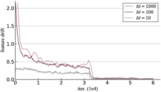
Figure 3: Feature drift with different steps on SOP. The embeddings of training instances drift within a relatively small distance even under a large interval, e.g. $\Delta t=1000$.

Furthermore, we demonstrate that such “slow drift” phenomena can provide a strict upper bound for the error of gradients of a pair-based loss. For simplicity, we consider the contrastive loss of one single negative pair $\mathcal{L}={\bm{v}}_{i}^{T}{\bm{v}}_{j}$, where ${\bm{v}}_{i}$, ${\bm{v}}_{j}$ are the embeddings of current model and $\widetilde{{\bm{v}}}_{j}$ is an approximation of ${\bm{v}}_{j}$.

Lemma 1.

Assume $||{\bm{v}}_{j}-\widetilde{{\bm{v}}}_{j}||^{2}_{2}<\epsilon$ , $\widetilde{\mathcal{L}}={\bm{v}}_{i}^{T}\widetilde{{\bm{v}}}_{j}$ and $f$ satisfies Lipschitz continuous condition, then the error of gradients related to ${\bm{v}}_{i}$ is,

$$\Big{|}\Big{|}\frac{\partial\mathcal{L}}{\partial{\bm{\theta}}}-\frac{\partial\widetilde{\mathcal{L}}}{\partial{\bm{\theta}}}\Big{|}\Big{|}^{2}_{2}<C\epsilon,$$ (3)

where $C$ is the Lipschitz constant.

Proof and discussion of Lemma 1 are provided in Supplementary Materials. Empirically, $C$ is often less than 1 with the backbones used in our experiments. Lemma 1 suggests that the error of gradients is controlled by the error of embeddings under Lipschitz assumption. Thus, the “slow drift” phenomenon ensures that mining across mini-batches can provide negative pairs with valid information for pair-based methods.

In addition, we discover that the “slow drift” of embeddings is not a special phenomena in DML, and also exists in other conventional tasks, as shown in Supplementary Materials.

3.3 Cross-Batch Memory Module

Algorithm 1 Pseudocode of XBM.

⬇

train network f conventionally with K epochs

initialize XBM as queue M

for x, y in loader: # x: data, y: labels

anchors = f.forward(x)

# memory update

enqueue(M, (anchors.detach(), y))

dequeue(M)

# compare anchors with M

sim = torch.matmul(anchors.transpose(), M.feats)

loss = pair_based_loss(sim, y, M.labels)

loss.backward()

optimizer.step()

 

We first describe our cross-batch memory (XBM) module, with model initialization and updating mechanism. Then we show that our memory module is easy to implement, can be directly integrated into existing pair-based DML framework as a plug-and-play module, by simply using several lines of codes (in Algorithm 1).

XBM. As the feature drift is relatively large at the early epochs, we warm up the neural networks with 1k iterations, allowing the model to reach a certain local optimal field where the embeddings become more stable. Then we initialize the memory module ${\mathbb{M}}$ by computing the features of a set of randomly sampled training images with the warm-up model. Formally, ${{\mathbb{M}}}=\{(\widetilde{{\bm{v}}}_{1},\widetilde{y}_{1}),(\widetilde{{\bm{v}}}_{2},\widetilde{y}_{2}),\dots,(\widetilde{{\bm{v}}}_{m},\widetilde{y}_{M})\}$, where $\widetilde{{\bm{v}}}_{i}$ is initialized as the embedding of the i-th sample ${\bm{x}}_{i}$, and $M$ is the memory size. We define a memory ratio as $R_{{\mathbb{M}}}\mathrel{\vbox{\hbox{\scriptsize.}\hbox{\scriptsize.}}}=M/N$, the ratio of memory size to the training size.

We maintain and update our XBM module as a queue: at each iteration, we enqueue the embeddings and labels of the current mini-batch, and dequeue the entities of the earliest mini-batch. Thus our memory module is updated with embeddings of the current mini-batch directly, without any additional computation. Furthermore, the whole training set can be cached in the memory module, because very limited memory is required for storing the embedding features, e.g. $512$-$d$ float vectors. See the other update strategy in Supplementary Materials.

XBM augmented Pair-based DML. We perform hard negative mining with our XBM on the pair-based DML. For a pair-based loss, based on GPW in [37], it can be cast into a unified weighting formulation of pair-wise similarities within a mini-batch in Eqn.(1), where a similarity matrix is computed within a mini-batch, ${\bm{S}}$. To perform our XBM mechanism, we simply compute a cross-batch similarity matrix $\widetilde{{\bm{S}}}$ between the instances of current mini-batch and the memory bank.

Formally, the memory augmented pair-based DML can be formulated as below:

$$\small\mathcal{L}=\frac{1}{m}\sum_{i=1}^{m}\mathcal{L}_{i}=\sum_{i=1}^{m}\left[\sum_{\widetilde{y}_{j}\neq y_{i}}^{M}w_{ij}\widetilde{{\bm{S}}}_{ij}-\sum_{\widetilde{y}_{j}=y_{i}}^{M}w_{ij}\widetilde{{\bm{S}}}_{ij}\right],$$ (4)

where $\widetilde{{\bm{S}}}_{ij}={\bm{v}}_{i}^{T}\widetilde{{\bm{v}}}_{j}$. The memory augmented pair-based loss in Eqn.(4) is in the same form as the normal pair-based loss in Eqn.(1), by computing a new similarity matrix $\widetilde{{\bm{S}}}$. Each instance in current mini-batch is compared with all the instances stored in the memory, enabling us to collect sufficient informative pairs for training. The gradient of the loss $\mathcal{L}_{i}$ w.r.t. ${\bm{v}}_{i}$ is,

$$\frac{\partial\mathcal{L}_{i}}{\partial{\bm{v}}_{i}}=\sum_{\widetilde{y}_{j}\neq y_{i}}^{M}w_{ij}\widetilde{{\bm{v}}}_{j}-\sum_{\widetilde{y}_{j}=y_{i}}^{M}w_{ij}\widetilde{{\bm{v}}}_{j}$$ (5)

and the gradients w.r.t. ${\bm{v}}_{i}$ model parameters (${\bm{\theta}}$) can be computed through a chain rule:

$$\frac{\partial\mathcal{L}_{i}}{\partial{\bm{\theta}}}=\frac{\partial\mathcal{L}_{i}}{\partial{\bm{v}}_{i}}\frac{\partial{\bm{v}}_{i}}{\partial{\bm{\theta}}}$$ (6)

Finally, the model parameters ${\bm{\theta}}$ are optimized through stochastic gradient descent. Lemma 1 ensures that the gradient error raised by embedding drift can be strictly constrained with a bound, which minimizes the side effect to the model training.

Hard Mining Ability. We investigate the hard mining ability of our XBM mechanism. We study the amount of valid negative pairs produced by our memory module at each iteration. A negative pair with non-zero gradient is considered as valid. The statistical result is illustrated in Figure 4. Throughout the training procedure, our memory module steadily contributes about 1,000 hard negative pairs per iteration, whereas less than 10 valid pairs are generated by the original mini-batch mechanism.

Qualitative hard mining results are shown in Figure 5. Given a bicycle image as an anchor, the mini-batch provides limited and different images, e.g. roof and sofa, as negatives. On the contrary, our XBM offers both semantically bicycle-related images and other samples, e.g. wheel and clothes. These results clearly demonstrate that the proposed XBM can provide diverse, related, and even fine-grained samples to construct negative pairs.

Our results confirm that (1) existing pair-based approaches suffer from the problem of lacking informative negative pairs to learn a discriminative model, and (2) our XBM module can significantly strengthen the hard mining ability of pair-based DML in a very simple yet efficient manner. See more examples in Supplementary Materials.

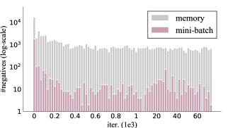
Figure 4: The number of valid negative examples from mini-batch and that from memory per iteration. Model is trained on SOP with $R_{M}=1$, mini-batch size 64 and GoogleNet as the backbone.

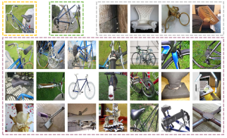
Figure 5: Given an anchor image ( yellow), examples of positive ( green) and negative from mini-batch ( gray) and that from memory ( purple). Current mini-batch can only bring few valid negatives with less information, while our XBM module can provide a wide variety of informative negative examples.

4 Experiments and Results

4.1 Implementation Details

We follow the standard settings in [22, 30, 23, 14] for fair comparison. Specifically, we adopt GoogleNet [33] as the default backbone network if not mentioned. The weights of the backbone were pre-trained on ILSVRC 2012-CLS dataset [27]. A 512-d fully-connected layer with $l_{2}$ normalization is added after the global pooling layer. The default embedding dimension is set as 512. For all datasets, the input images are first resized to $256\times 256$, and then cropped to $224\times 224$. Random crops and random flips are utilized as data augmentation during training. For testing, we only use the single center crop to compute the embedding for each instance as [22]. In all experiments, we use the Adam optimizer [15] with $5e^{-4}$ weight decay and the PK sampler (P categories, K samples/category) to construct mini-batches.

4.2 Datasets

Our methods are evaluated on three large-scale datasets for few-shot image retrieval. Recall$@k$ is reported. The training and testing protocol follow the standard setups:

Stanford Online Products (SOP) [22] contains 120,053 online product images in 22,634 categories. There are only 2 to 10 images for each category. Following [22], we use 59,551 images (11,318 classes) for training, and 60,502 images (11,316 classes) for testing.

In-shop Clothes Retrieval (In-shop) contains 72,712 clothing images of 7,986 classes. Following [20], we use 3,997 classes with 25,882 images as the training set. The test set is partitioned to a query set with 14,218 images of 3,985 classes, and a gallery set having 3,985 classes with 12,612 images.

PKU VehicleID (VehicleID) [19] contains 221,736 surveillance images of 26,267 vehicle categories, where 13,134 classes (110,178 images) are used for training. Following the test protocol described in [19], evaluation is conducted on a predefined small, medium and large test sets which contain 800 classes (7,332 images), 1600 classes (12,995 images) and 2400 classes (20,038 images) respectively.

	SOP				In-shop						VehicleID
											Small		Medium		Large
Recall$@K$ (%)	1	10	100	1000	1	10	20	30	40	50	1	5	1	5	1	5
Contrastive	64.0	81.4	92.1	97.8	77.1	93.0	95.2	96.1	96.8	97.1	79.5	91.6	76.2	89.3	70.0	86.0
Contrastive w/ M	77.8	89.8	95.4	98.5	89.1	97.3	98.1	98.4	98.7	98.8	94.1	96.2	93.1	95.5	92.5	95.5
Triplet	61.6	80.2	91.6	97.7	79.8	94.8	96.5	97.4	97.8	98.2	86.9	94.8	84.8	93.4	79.7	91.4
Triplet w/ M	74.2	87.4	94.2	98.0	82.9	95.7	96.9	97.4	97.8	98.0	93.3	95.8	92.0	95.0	91.3	94.8
MS	69.7	84.2	93.1	97.9	85.1	96.7	97.8	98.3	98.7	98.8	91.0	96.1	89.4	94.8	86.7	93.8
MS w/ M	76.2	89.3	95.4	98.6	87.1	97.1	98.0	98.4	98.7	98.9	94.1	96.7	93.0	95.8	92.1	95.6

Table 1: Retrieval results of memory augmented (‘w/ M’) pair-based methods compared with their respective baselines on three datasets.

4.3 Ablation Study

We provide ablation study on SOP dataset with GoogleNet to verify the effectiveness of our XBM module.

Memory Ratio. The search space of our cross-batch hard mining can be dynamically controlled by memory ratio $R_{{\mathbb{M}}}$. We illustrate the impact of memory ratio to XBM augmented contrastive loss on three benchmarks (in Figure 1, right). Firstly, our method significantly outperforms the baseline (with $R_{{\mathbb{M}}}=0$), with over 20% improvements on all three datasets using various configurations of $R_{{\mathbb{M}}}$. Secondly, our method with mini-batch of 16 can achieve better performance than the non-memory counterpart using 256 mini-batch, e.g. with an improvement of 71.7%$\rightarrow$78.2% on recall@1, while saving GPU memory considerably.

More importantly, our XBM can boost the contrastive loss largely with small $R_{{\mathbb{M}}}$ (e.g. on In-shop, 52.0%$\rightarrow$ 79.4% on recall@1 with $R_{{\mathbb{M}}}=0.01$) and its performance is going to be saturated when the memory expands to a moderate size. It makes sense, since the memory with a small $R_{{\mathbb{M}}}$ (e.g. 1%) already contains thousands of embeddings to generate sufficient valid negative instances on large-scale datasets, especially fine-grained ones, such as In-shop or VehicleID. Therefore, our memory scheme can have consistent and stable performance improvements with a wide range of memory ratios.

Mini-batch Size. Mini-batch size is critical to the performance of many pair-based approaches (Figure 1, left). We further investigate its impact to our memory augmented pair-based methods (shown in Figure 6). Our method has a 3.2% performance gain by increasing its mini-batch size from 16 to 256, while the original contrastive method has a significantly larger improvement of 25.1%. Obviously, with the proposed memory module, the impact of mini-batch size is reduced significantly. This indicates that the effect of mini-batch size can be strongly compensated by our memory module, which provides a more principled solution to address the hard mining problem in DML.

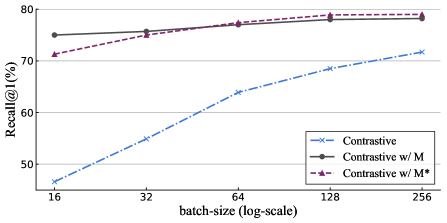
Figure 6: Performance of contrastive loss by training with different mini-batch sizes. Unlike conventional pair-based methods, XBM augmented contrastive loss is equally effective under random shuffle mini-batch sampler (denoted with superscript *).

With General Pair-based DML. Our memory module can be directly applied to the GPW framework. We evaluate it with contrastive loss, triplet loss and MS loss. As shown in Table 1, our memory module can improve the original DML approaches significantly and consistently on all benchmarks. Specifically, the memory module remarkably boosts the performance of contrastive loss by 64.0%$\rightarrow$77.8% and MS loss by 69.7%$\rightarrow$76.2%. Furthermore, with sophisticated sampling and weighting approach, MS loss has 16.7% recall@1 performance improvement over contrastive loss on VehicleID Large test set. Such a large gap can be simply filled by our memory module, with a further 5.8% improvement. MS loss has a smaller improvement because it weights extremely hard negatives heavily which might be outliers, while such a harmful influence is weakened by the equally weighting scheme of contrastive loss. For a detailed analysis see Supplementary Materials (SM).

The results suggest that (1) both straightforward (e.g. contrastive loss) and carefully designed weighting scheme (e.g. MS loss) can be improved largely by our memory module, and (2) with our memory module, a simple pair-weighting method (e.g. contrastive loss) can easily outperform the most sophisticated, state-of-the-art methods such as MS loss [37] by a large margin.

Method	Time	GPU Mem.	R@1	Gain
Cont. bs. 64	2.10 h.	5.12 GB	63.9	-
Cont. bs. 256	4.32 h.	+15.7 GB	71.7	+7.8
Cont. w/ 1% $R_{M}$	2.48 h.	+0.01 GB	69.8	+5.9
Cont. w/ 100% $R_{M}$	3.19 h.	+0.20 GB	77.4	+13.5

Table 2: Training time and GPU memory cost on 64, 256 mini-batch size and 1%, 100% memory ratio with 64 mini-batch size.

Memory and Computational Cost. We analyze the complexity of our XBM module on memory and computational cost. On memory cost, The XBM module ${\mathbb{M}}$ ($\mathcal{O}(DM)$) and affinity matrix $\widetilde{{\bm{S}}}$ ($\mathcal{O}(mM)$) requires a negligible 0.2 GB GPU memory for caching the whole training set (Table 2). On computational complexity, the cost of $\widetilde{{\bm{S}}}$ ($\mathcal{O}(mDM)$) increases linearly with memory size $M$. With a GPU implementation, it takes a reasonable 34% amount of extra training time w.r.t. the forward and backward procedure.

It is also worth noting that XBM does not act in the inference phase. It only requires 1 hour extra training time and 0.2GB memory, to achieve a surprising 13.5% performance gain by using a single GPU. Moreover, our method can be scalable to an extremely large-scale dataset, e.g. with 1 billion samples, since our XBM module can generate a rich set of valid negatives with a small-memory-ratio XBM, which requires acceptable cost.

4.4 Quantitative and Qualitative Results

In this section, we compare our XBM augmented contrastive loss with the state-of-the-art DML methods on three benchmarks on image retrieval. Even though our method can reach better performance with a larger mini-batch size (Figure 6), we only use 64 mini-batch which can be implemented on a single GPU with ResNet50 [11]. Since the backbone architecture and embedding dimension can effect the recall metric, we list the results of our method with various configurations for fair comparison in Table 3, 4 and 5. See results on more datasets in SM.

The results demonstrate that our XBM module, with a contrastive loss, can surpass the state-of-the-art methods on all datasets by a large margin. On SOP, our method with R${}^{\text{128}}$ outperforms the current state-of-the-art method: MIC [26] by 77.2% $\rightarrow$ 80.6%. On In-shop, our method with R${}^{\text{128}}$ achieves even higher performance than FastAP [2] with R${}^{\text{512}}$, and improves by 88.2%$\rightarrow$91.3% compared to MIC. On VehicleID, our method outperforms existing approaches considerably. For example, on the large test dataset, by using a same G${}^{\text{512}}$, it improves the R@1 of recent A-BIER [24] largely by 81.9%$\rightarrow$92.5%. With R${}^{\text{128}}$, our method surpasses the best results by 87%$\rightarrow$93%, which is obtained by FastAP [2] using R${}^{\text{512}}$.

Figure 7 shows that our memory module promotes the learning of a more discriminative encoder. For example, at the first row, our model is aware of the deer under the lamp which is a specific character of the query product, and retrieves the correct images. In addition, we also present some bad cases in the bottom rows, where our retrieved results are visually closer to the query than that of baseline model. See more visualizations in SM.

Recall$@K$ (%)		1	10	100	1000
HDC [45]	G${}^{\text{384}}$	69.5	84.4	92.8	97.7
A-BIER [24]	G${}^{\text{512}}$	74.2	86.9	94.0	97.8
ABE [14]	G${}^{\text{512}}$	76.3	88.4	94.8	98.2
SM [32]	G${}^{\text{512}}$	75.2	87.5	93.7	97.4
Clustering [31]	B${}^{\text{64}}$	67.0	83.7	93.2	-
ProxyNCA [21]	B${}^{\text{64}}$	73.7	-	-	-
HTL [6]	B${}^{\text{512}}$	74.8	88.3	94.8	98.4
MS [37]	B${}^{\text{512}}$	78.2	90.5	96.0	98.7
SoftTriple [25]	B${}^{\text{512}}$	78.6	86.6	91.8	95.4
Margin [40]	R${}^{\text{128}}$	72.7	86.2	93.8	98.0
Divide [28]	R${}^{\text{128}}$	75.9	88.4	94.9	98.1
FastAP [2]	R${}^{\text{128}}$	73.8	88.0	94.9	98.3
MIC [26]	R${}^{\text{128}}$	77.2	89.4	95.6	-
Cont. w/ M	G${}^{\text{512}}$	77.4	89.6	95.4	98.4
Cont. w/ M	B${}^{\text{512}}$	79.5	90.8	96.1	98.7
Cont. w/ M	R${}^{\text{128}}$	80.6	91.6	96.2	98.7

Table 3: Recall@$K(\%)$ performance on SOP. ‘G’, ‘B’ and ‘R’ denotes applying GoogleNet, InceptionBN and ResNet50 as backbone respectively, and the superscript is embedding size.

Recall$@K$ (%)		1	10	20	30	40	50
HDC [45]	G${}^{\text{384}}$	62.1	84.9	89.0	91.2	92.3	93.1
A-BIER [24]	G${}^{\text{512}}$	83.1	95.1	96.9	97.5	97.8	98.0
ABE [14]	G${}^{\text{512}}$	87.3	96.7	97.9	98.2	98.5	98.7
HTL [6]	B${}^{\text{512}}$	80.9	94.3	95.8	97.2	97.4	97.8
MS [37]	B${}^{\text{512}}$	89.7	97.9	98.5	98.8	99.1	99.2
Divide [28]	R${}^{\text{128}}$	85.7	95.5	96.9	97.5	-	98.0
MIC [26]	R${}^{\text{128}}$	88.2	97.0	-	98.0	-	98.8
FastAP [2]	$R^{\text{512}}$	90.9	97.7	98.5	98.8	98.9	99.1
Cont. w/ M	G${}^{\text{512}}$	89.4	97.5	98.3	98.6	98.7	98.9
Cont. w/ M	B${}^{\text{512}}$	89.9	97.6	98.4	98.6	98.8	98.9
Cont. w/ M	R${}^{\text{128}}$	91.3	97.8	98.4	98.7	99.0	99.1

Table 4: Recall@$K(\%)$ performance on In-Shop.

Method		Small		Medium		Large
		1	5	1	5	1	5
GS-TRS [5]		75.0	83.0	74.1	82.6	73.2	81.9
BIER [23]	G${}^{\text{512}}$	82.6	90.6	79.3	88.3	76.0	86.4
A-BIER [24]	G${}^{\text{512}}$	86.3	92.7	83.3	88.7	81.9	88.7
VANet [4]	G${}^{\text{2048}}$	83.3	95.9	81.1	94.7	77.2	92.9
MS [37]	B${}^{\text{512}}$	91.0	96.1	89.4	94.8	86.7	93.8
Divide [28]	R${}^{\text{128}}$	87.7	92.9	85.7	90.4	82.9	90.2
MIC [26]	R${}^{\text{128}}$	86.9	93.4	-	-	82.0	91.0
FastAP [2]	$R^{\text{512}}$	91.9	96.8	90.6	95.9	87.5	95.1
Cont. w/ M	G${}^{\text{512}}$	94.0	96.3	93.2	95.4	92.5	95.5
Cont. w/ M	B${}^{\text{512}}$	94.6	96.9	93.4	96.0	93.0	96.1
Cont. w/ M	R${}^{\text{128}}$	94.7	96.8	93.7	95.8	93.0	95.8

Table 5: Recall@$K(\%)$ performance on VehicleID.

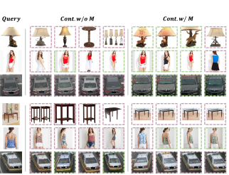
Figure 7: Top 4 retrieved images w/o and w/ memory module. Correct results are highlighted with green, while incorrect purple.

5 Conclusions

We have presented a conceptually simple, easy to implement, and memory efficient cross-batch mining mechanism for pair-based DML. In this work, we identify the “slow drift” phenomena that the embeddings drift exceptionally slow during the training process. Then we propose a cross-batch memory (XBM) module to dynamically update the embeddings of instances of recent mini-batches, which allows us to collect sufficient hard negative pairs across multiple mini-batches, or even from the whole dataset. Without bells and whistles, the proposed XBM can be directly integrated into a general pair-based DML framework, and improve the performance of existing pair-based methods significantly on image retrieval. In particular, with our XBM, a contrastive loss can easily surpass state-of-the-art methods [37, 26, 2] by a large margin on three large-scale datasets.

This paves a new path in solving for hard negative mining which is a fundamental problem for various computer vision tasks. Furthermore, we hope that the dynamic memory mechanism can be extended to improve a wide variety of machine learning tasks because ”slow drift” is a general phenomenon not only occurring in DML.

See pages 1 of supplementary.pdf See pages 2 of supplementary.pdf See pages 3 of supplementary.pdf See pages 4 of supplementary.pdf See pages 5 of supplementary.pdf See pages 6 of supplementary.pdf See pages 7 of supplementary.pdf See pages 8 of supplementary.pdf

References

- [1] Maxime Bucher, Stéphane Herbin, and Frédéric Jurie. Improving semantic embedding consistency by metric learning for zero-shot classiffication. In ECCV, 2016.
- [2] Fatih Cakir, Kun He, Xide Xia, Brian Kulis, and Stan Sclaroff. Deep metric learning to rank. In CVPR, 2019.
- [3] S. Chopra, R. Hadsell, and Y. LeCun. Learning a similarity metric discriminatively, with application to face verification. In CVPR, 2005.
- [4] Ruihang Chu, Yifan Sun, Yadong Li, Zheng Liu, Chi Zhang, and Yichen Wei. Vehicle re-identification with viewpoint-aware metric learning. In ICCV, 2019.
- [5] Yan Em, Feng Gag, Yihang Lou, Shiqi Wang, Tiejun Huang, and Ling-Yu Duan. Incorporating intra-class variance to fine-grained visual recognition. In ICME. IEEE, 2017.
- [6] Weifeng Ge, Weilin Huang, Dengke Dong, and Matthew R Scott. Deep metric learning with hierarchical triplet loss. In ECCV, 2018.
- [7] Alexander Grabner, Peter M. Roth, and Vincent Lepetit. 3d pose estimation and 3d model retrieval for objects in the wild. In CVPR, 2018.
- [8] R. Hadsell, S. Chopra, and Y. LeCun. Dimensionality reduction by learning an invariant mapping. In CVPR, 2006.
- [9] Ben Harwood, Vijay Kumar B G, Gustavo Carneiro, Ian Reid, and Tom Drummond. Smart mining for deep metric learning. In ICCV, 2017.
- [10] Kaiming He, Haoqi Fan, Yuxin Wu, Saining Xie, and Ross Girshick. Momentum contrast for unsupervised visual representation learning. In arXiv:1911.05722, 2019.
- [11] Kaiming He, Xiangyu Zhang, Shaoqing Ren, and Jian Sun. Deep residual learning for image recognition. In CVPR, 2016.
- [12] Xinwei He, Yang Zhou, Zhichao Zhou, Song Bai, and Xiang Bai. Triplet-center loss for multi-view 3d object retrieval. In CVPR, 2018.
- [13] Alexander Hermans*, Lucas Beyer*, and Bastian Leibe. In defense of the triplet loss for person re-identification. arXiv:1703.07737v4, 2017.
- [14] Wonsik Kim, Bhavya Goyal, Kunal Chawla, Jungmin Lee, and Keunjoo Kwon. Attention-based ensemble for deep metric learning. In ECCV, 2018.
- [15] Diederick P Kingma and Jimmy Ba. Adam: A method for stochastic optimization. In ICLR, 2015.
- [16] Sasi Kiran Yelamarthi, Shiva Krishna Reddy, Ashish Mishra, and Anurag Mittal. A zero-shot framework for sketch based image retrieval. In ECCV, 2018.
- [17] Laura Leal-Taixé, Cristian Canton-Ferrer, and Konrad Schindler. Learning by tracking: Siamese cnn for robust target association. In CVPR Workshops, 2016.
- [18] Suichan Li, Dapeng Chen, Bin Liu, Nenghai Yu, and Rui Zhao. Memory-based neighbourhood embedding for visual recognition. In ICCV, 2019.
- [19] Hongye Liu, Yonghong Tian, Yaowei Wang, Lu Pang, and Tiejun Huang. Deep relative distance learning: Tell the difference between similar vehicles. In CVPR, 2016.
- [20] Ziwei Liu, Ping Luo, Shi Qiu, Xiaogang Wang, and Xiaoou Tang. Deepfashion: Powering robust clothes recognition and retrieval with rich annotations. In CVPR, 2016.
- [21] Yair Movshovitz-Attias, Alexander Toshev, Thomas K. Leung, Sergey Ioffe, and Saurabh Singh. No fuss distance metric learning using proxies. In ICCV, 2017.
- [22] Hyun Oh Song, Yu Xiang, Stefanie Jegelka, and Silvio Savarese. Deep metric learning via lifted structured feature embedding. In CVPR, 2016.
- [23] Michael Opitz, Georg Waltner, Horst Possegger, and Horst Bischof. Bier - boosting independent embeddings robustly. In ICCV, 2017.
- [24] Michael Opitz, Georg Waltner, Horst Possegger, and Horst Bischof. Deep metric learning with bier: Boosting independent embeddings robustly. PAMI, 2018.
- [25] Qi Qian, Lei Shang, Baigui Sun, and Juhua Hu. Softtriple loss: Deep metric learning without triplet sampling. ICCV, 2019.
- [26] Karsten Roth, Biagio Brattoli, and Bjorn Ommer. Mic: Mining interclass characteristics for improved metric learning. In ICCV, 2019.
- [27] Olga Russakovsky, Jia Deng, Hao Su, Jonathan Krause, Sanjeev Satheesh, Sean Ma, Zhiheng Huang, Andrej Karpathy, Aditya Khosla, Michael Bernstein, Alexander C. Berg, and Li Fei-Fei. ImageNet Large Scale Visual Recognition Challenge. IJCV, 2015.
- [28] Artsiom Sanakoyeu, Vadim Tschernezki, Uta Buchler, and Bjorn Ommer. Divide and conquer the embedding space for metric learning. In CVPR, 2019.
- [29] Florian Schroff, Dmitry Kalenichenko, and James Philbin. Facenet: A unified embedding for face recognition and clustering. In CVPR, 2015.
- [30] Kihyuk Sohn. Improved deep metric learning with multi-class n-pair loss objective. In NeurIPS. 2016.
- [31] Hyun Oh Song, Stefanie Jegelka, Vivek Rathod, and Kevin Murphy. Deep metric learning via facility location. In CVPR, 2017.
- [32] Yumin Suh, Bohyung Han, Wonsik Kim, and Kyoung Mu Lee. Stochastic class-based hard example mining for deep metric learning. In CVPR, 2019.
- [33] Christian Szegedy, Wei Liu, Yangqing Jia, Pierre Sermanet, Scott Reed, Dragomir Anguelov, Dumitru Erhan, Vincent Vanhoucke, and Andrew Rabinovich. Going deeper with convolutions. In CVPR, 2015.
- [34] Ran Tao, Efstratios Gavves, and Arnold WM Smeulders. Siamese instance search for tracking. In CVPR, 2016.
- [35] Evgeniya Ustinova and Victor Lempitsky. Learning deep embeddings with histogram loss. In NeurIPS. 2016.
- [36] Oriol Vinyals, Charles Blundell, Timothy Lillicrap, Daan Wierstra, et al. Matching networks for one shot learning. In NeurIPS, 2016.
- [37] Xun Wang, Xintong Han, Weilin Huang, Dengke Dong, and Matthew R Scott. Multi-similarity loss with general pair weighting for deep metric learning. In CVPR, 2019.
- [38] Yandong Wen, Kaipeng Zhang, Zhifeng Li, and Yu Qiao. A discriminative feature learning approach for deep face recognition. In ECCV, 2016.
- [39] Paul Wohlhart and Vincent Lepetit. Learning descriptors for object recognition and 3d pose estimation. In CVPR, 2015.
- [40] Chao-Yuan Wu, R. Manmatha, Alexander J. Smola, and Philipp Krähenbühl. Sampling matters in deep embedding learning. ICCV, 2017.
- [41] Zhirong Wu, Alexei A Efros, and Stella Yu. Improving generalization via scalable neighborhood component analysis. In ECCV, 2018.
- [42] Zhirong Wu, Yuanjun Xiong, Stella X Yu, and Dahua Lin. Unsupervised feature learning via non-parametric instance discrimination. In CVPR, pages 3733–3742, 2018.
- [43] Tong Xiao, Shuang Li, Bochao Wang, Liang Lin, and Xiaogang Wang. Joint detection and identification feature learning for person search. In CVPR, 2017.
- [44] Rui Yu, Zhiyong Dou, Song Bai, Zhaoxiang Zhang, Yongchao Xu, and Xiang Bai. Hard-aware point-to-set deep metric for person re-identification. In ECCV, 2018.
- [45] Yuhui Yuan, Kuiyuan Yang, and Chao Zhang. Hard-aware deeply cascaded embedding. In ICCV, 2017.
- [46] Andrew Zhai, Hao-Yu Wu, and US San Francisco. Classification is a strong baseline for deep metric learning. 2019.
- [47] Ziming Zhang and Venkatesh Saligrama. Zero-shot learning via joint latent similarity embedding. In CVPR, 2016.
- [48] Zhun Zhong, Liang Zheng, Zhiming Luo, Shaozi Li, and Yi Yang. Invariance matters: Exemplar memory for domain adaptive person re-identification. In CVPR, 2019.