Efficient Per-Example Gradient Computations in
Convolutional Neural Networks

Abstract

Deep learning frameworks leverage GPUs to perform massively-parallel computations over batches of many training examples efficiently. However, for certain tasks, one may be interested in performing per-example computations, for instance using per-example gradients to evaluate a quantity of interest unique to each example. One notable application comes from the field of differential privacy, where per-example gradients must be norm-bounded in order to limit the impact of each example on the aggregated batch gradient. In this work, we discuss how per-example gradients can be efficiently computed in convolutional neural networks (CNNs). We compare existing strategies by performing a few steps of differentially-private training on CNNs of varying sizes. We also introduce a new strategy for per-example gradient calculation, which is shown to be advantageous depending on the model architecture and how the model is trained. This is a first step in making differentially-private training of CNNs practical.

1 Introduction

Today, as developments have progressed in the field of privacy-aware machine learning (ML), it has become widely acknowledged that applying ML to sensitive data introduces a number of privacy risks which must be taken into consideration when building responsible ML systems. Multiple works [1, 2, 3, 4] have shown that some information about training data can be recovered from the network’s parameters, especially in the context of membership inference. To be able to use sensitive data such as medical records for training machine learning models, something must be done to ensure the privacy of the data with respect to the trained model. One approach to this is differential privacy (DP) [5], which limits the influence that one specific data point can have on the model parameters. In the case of ML applied to medical records, the utility in applying DP would be to provide a mathematical assurance on the level of potential additional harm that could come to a patient if their records are included in the training cohort rather than excluded.

A necessary step in the application of DP to the training of ML models via stochastic gradient descent, as shown in [6], is the application of gradient clipping. Notably, model gradients must be norm-bounded individually for each sample, not according to the aggregate across a given mini-batch. That is, one should consider the gradient of the loss $\mathcal{L}_{i}$ induced by example $i$, rather than the gradient of the global loss $\sum_{i}\mathcal{L}_{i}$. This per-example gradient clipping has also been used in the context of reinforcement learning [7]. In [6], gradient clipping is defined for a given maximum gradient norm bound $C$ by

$$\bar{g}(x_{i})=\frac{g(x_{i})}{\max\left(1,\frac{1}{C}||g(x_{i})||_{2}\right)},$$ (1)

where $g(x_{i})\triangleq\nabla_{\theta}\mathcal{L}_{i}(\theta,x_{i})$ is the gradient of the model parameters with respect to data input $x_{i}$. This gradient clipping has the effect of bounding the maximal amount of influence a single sample can have on the direction of a model update. When applied over the course of training, in conjunction with the addition of noise, the sensitivity of the final model to any one sample is therefore bounded thanks to the composition properties of DP [6].

Unfortunately, auto-differentiation libraries, like those included in PyTorch and Tensorflow, do not naturally offer the option to compute per-example gradients as conventional ML training workflows only require a single gradient produced by averaging across the samples of the mini-batch. Since a successful implementation of differentially-private model training requires this per-example gradient clipping, efficiently producing per-example gradients is a critical step. One approach would be to start from the bottom and make the necessary changes to existing low-level auto-differentiation tools to enable this computation. Another tactic, which we investigate here, is to start from the high-level framework API (in this case, PyTorch) and see what options are available to effect this per-example gradient estimation.

Multiple methods in this vein have been suggested over the past several years. One such method was introduced by Goodfellow in a technical report [8]. While very efficient, this method only applies to linear fully-connected (dense) network layers. In this report, we explain how to extend the approach of [8] to convolutional networks, and proceed to compare its efficiency to that of other existing approaches.

2 Existing methods for computing per-example gradients

In this section, we review some of the existing techniques for computing per-example gradients at the level of the of the ML framework API. Algorithmic optimization can accelerate the computation, but the main speed-ups come from fully utilizing the parallelization of operations on GPU. The three main approaches to per-example gradient computation are described as follows:

Naive approach.

The simplest strategy consists in changing the batch size to $1$. Doing so, one can iterate over the originally desired batch size, computing the gradient corresponding to each sample in the batch. Since there is no parallelization, this method is very slow. This approach requires a minimal amount of code. We denote it by naive in our experiments.

Changing one step of the backpropagation.

In [8], it was shown that one can use the auto-differentiation’s intermediate results to compute the per-example gradient by hand. However, this formulation does not allow for convolutions to be used efficiently. In practice, when attempting to apply DP to training Deep Convolutional Neural Networks (DCNN) models, multiple papers have used a transfer learning approach, training only the last linear task layers while freezing a set of pre-trained CNN feature extraction layers [6, 9, 10]. We explain in the next section how to extend this computation to CNNs using functions available in PyTorch. We denote it by crb in our experiments, for chain rule based.

Using multiple copies of the model.

This strategy relies on the same idea as the first one: using mini-batches of size 1. In this approach, however, one copies the model as many times as there are samples in the batch. Each model is used on only one example, thus parallelizing the iteration from the first approach. This approach is very fast and requires only a small amount of code. In addition to this, the model duplicates can share their parameters with the original model in order to minimize the training memory footprint. This method has been proposed by Goodfellow in 2017, on a Github thread. We denote it by multi in our experiments.

3 Per-example backpropagation for convolutional networks

In this section, we describe a way to compute per-example gradients from partial derivatives explicitly computed by auto-differentiation tools. We only describe the computation of these gradients for a single linear layer, but the extension to multiple non-linear layers is straightforward. Doing so for each layer in the network results in full per-example gradients. This method is denoted crb in our experiments, which stands for chain rule based. We provide an implementation of this method at https://github.com/owkin/grad-cnns.

3.1 Fully-connected linear layers

In the case of dense linear layers, one can refer directly to the technique introduced in [8], which we reproduce, here. Let $H$ be a linear layer of a neural network, with input $x=\left[x_{1},\ldots,x_{I}\right]^{T}$ and output $y=Hx=\left[y_{1},\ldots,y_{J}\right]^{T}$. When training a model, we wish to update the model parameters $H$ so as to minimize some output-depending loss function $\mathcal{L}$, i.e. following the negative gradient of $\mathcal{L}$ w.r.t. $H$. This gradient is obtained from the model output via backpropagation,

$$\frac{\partial\mathcal{L}}{\partial H_{kl}}=\sum_{j}\frac{\partial y_{j}}{\partial H_{kl}}\,\frac{\partial\mathcal{L}}{\partial y_{j}}=x_{l}\,\frac{\partial\mathcal{L}}{\partial y_{k}}\,.$$ (2)

The trick of calculating per-example gradients post auto-differentiation comes from the observation of the final equality above: the partial w.r.t. a single coefficient of $H$ comes from the simple multiplication of a single layer input with the partial of the loss with respect to a single output. As noted by [8], one can store the layer’s input $x$, and auto-differentiation tools give access to $\frac{\partial\mathcal{L}}{\partial y}$ for each sample in the batch. We can then compute the gradient with simple batch matrix multiplications, an outer-product computation, which can be done efficiently on GPU, $\nabla_{H}\mathcal{L}=(\nabla_{y}\mathcal{L})\,x^{T}$.

3.2 Application to convolutional layers

The computation described above uses linear matrix representation, which if applied to the case of convolution would be extremely inefficient. We describe in this section how to use convolution operations to obtain the same result when back-propagating through convolutional layers. We will do so using PyTorch format for tensors dimensions, i.e. (batch, channels, spatial dimensions).

3.2.1 Notation

Spatial dimensions.

In order not to overcomplicate the derivation, we will work with 1D convolutions. We will refer to this spatial dimension with the variable $t\in\{0\ldots T-1\}$, or in the case of the convolutional kernel, with the letter $k\in\{0\ldots K-1\}$. Note that the same derivations are correct for other dimensions.

Channels.

Channels will be an essential part of our derivation, especially when dealing with the groups argument. We will refer to the input and output channels respectively with the variables $c\in\{0\ldots C-1\}$ and $d\in\{0\ldots D-1\}$.

Batch.

We will refer to the batch dimension with the variable $b\in\{0\ldots B-1\}$.

3.2.2 Standard convolution

We start with standard convolution as implemented in most ML frameworks; a set of filters, or kernels, $h$ of shape $(D,C,K)$ is convolved with the input tensor $x$ of shape $(B,C,T)$ to form an output tensor $y$ of shape $(B,D,T-K+1)$. This discrete convolution is given by the formula

$$y[b,d,t]=(x\ast h)[b,d,t]\triangleq\sum_{c=0}^{C-1}\sum_{k=0}^{K-1}x[b,c,t+k]\,h[d,c,k]\,,$$ (3)

where we note the aggregation step performed over the $C$ input channels to produce the final convolved output of the layer. To calculate per-example gradients with respect to $h$, we are interested in differentiating sample $b$’s contribution to the loss $\mathcal{L}$, that is, $\mathcal{L}[b]$ where $\mathcal{L}=\sum_{b}\mathcal{L}[b]$. By applying the same technique as in the fully-connected case, but carrying through the convolution operation, we see that the gradient with respect to the convolution kernel is

$$\frac{\partial\mathcal{L}[b]}{\partial h[d,c,k]} =\sum_{t=0}^{T-K}\frac{\partial y[b,d,t]}{\partial h[d,c,k]}\,\frac{\partial\mathcal{L}[b]}{\partial y[b,d,t]}$$

$$=\sum_{t=0}^{T-K}\frac{\partial\left(\sum_{\tilde{c}=0}^{C-1}\sum_{\tilde{k}=0}^{K-1}x[b,\tilde{c},t+\tilde{k}]\,h[d,\tilde{c},\tilde{k}]\right)}{\partial h[d,c,k]}\,\frac{\partial\mathcal{L}[b]}{\partial y[b,d,t]}$$

$$=\sum_{t=0}^{T-K}x[b,c,t+k]\,\underbrace{\frac{\partial\mathcal{L}[b]}{\partial y[b,d,t]}}_{\nabla_{y}\mathcal{L}[b,d,t]}\,.$$

Since the spatial dimensions of $x$ and $\nabla_{y}\mathcal{L}$ are $T$ and $T-K+1$ respectively, their convolution has the same spatial dimension $K$ as the convolution kernel. This convolution can be seen as a per-example convolution, which we denote by $\circledast$:

$$\frac{\partial\mathcal{L}[b]}{\partial h[d,c,k]}=\left(x\circledast\nabla_{y}\mathcal{L}\right)[b,d,c,k]\,\triangleq\sum_{t=0}^{T-K}x[b,c,t+k]\,\nabla_{y}\mathcal{L}[b,d,t].$$ (4)

This convolution operation, although similar to the one in (3), is not available in auto-differentiation libraries. However, the groups argument in PyTorch’s regular convolution allows one to evaluate such an operation. Recall that groups splits the input tensor into groups of the same size, performs independent convolutions on each group, and finally concatenates the resulting outputs. More precisely, one can reshape the input $x$ to size $(B,C/G,G,T)$, and the kernel $h$ to $(D/G,G,C/G,K)$ and subsequently define the group convolution as

$$\forall d\in\{0\ldots D/G-1\},\quad y[b,g\frac{D}{G}+d,t]=(x\ast_{G}h)[b,d,g,t]\triangleq\sum_{c=0}^{C/G-1}\sum_{k=0}^{K-1}x[b,c,g\frac{C}{G}+c,t+k]\,h[d,g,c,k].$$ (5)

In Algorithm 1, we explain how to use the group convolution (5) in order to evaluate (4). We first replace $h$ by $\nabla_{y}\mathcal{L}$ in the formula above, and swap $t$ and $k$, also making sure that $K$ is set to $T-K+1$. Axes are then swapped and/or combined in such a way that (4) is recovered. Namely, $x$ is reshaped to $(1,B,C,T)$, so that the effective batch size is 1 and the number of input channels is $B$; and $\nabla_{y}\mathcal{L}$ is reshaped to $(BD,1,1,T-K+1)$, so that the number of output channels is $BD$. The key is in noting that, since each sample is treated as a different input channel, grouping allows us to treat each of them in parallel. Finally, we note that after reshaping the inputs to the convolution, it is necessary, even though we operate on a 1D spatial dimension, to utilize a 2D convolution. Analogously, when adapting this procedure to the estimation of per-example gradients for 2D convolutional layers, it is necessary to use a 3D convolution.

Input: $x$ of size $(B,C,T)$, $\delta y\triangleq\nabla_{y}\mathcal{L}$ of size $(B,D,T-K+1)$

Result: $\delta h\triangleq\nabla_{h}\mathcal{L}$ of size $(B,D,C,K)$

# Reshape $x$ and $\delta y$

$x$ $\leftarrow$ reshape $x$ to shape $(1,B,C,T)$

$\delta y$ $\leftarrow$ reshape $\delta y$ to shape $(B\times D,1,1,T-K+1)$

# Call regular convolution function, with one extra dimension

$\delta y$ $\leftarrow$ conv2d($x$, $\delta y$, groups=$B$)      # shape $(1,B\times D,C,K)$

# Reshape output

$\delta h$ $\leftarrow$ reshape $\delta h$ to shape $(B,D,C,K)$

return $\delta h$

Algorithm 1 Standard convolution: per-example gradients.

Input: $x$ of size $(B,C,T)$, $\delta y\triangleq\nabla_{y}\mathcal{L}$ of size $(B,D,T^{\prime})$, number of groups $\Gamma$, padding size $\Pi$, stride $\Sigma$ and dilation $\Delta$

Result: $\delta h\triangleq\nabla_{h}\mathcal{L}$ of size $(B,D,C,K)$

# Reshape $x$ and $y$

$x$ $\leftarrow$ reshape $x$ to shape $(1,B\times\Gamma,C/\Gamma,T)$

$\delta y$ $\leftarrow$ reshape $\delta y$ to shape $(B\times D,1,1,T^{\prime})$

# Define arguments for convolution with one extra spatial dimension

$\Gamma^{\prime}\leftarrow B\times\Gamma$

$\Pi^{\prime}\leftarrow(0,\Pi)$      # zero padding on extra dimension

$\Sigma^{\prime}\leftarrow(1,\Delta)$      # arguments $\Sigma$ and $\Delta$ are switched

$\Delta^{\prime}\leftarrow(1,\Sigma)$      # both arguments are one on extra dimension

# Call convolution function, with one extra dimension

$\delta h\leftarrow$ conv2d($x$, $\delta y$, groups=$\Gamma^{\prime}$, padding=$\Pi^{\prime}$, stride=$\Sigma^{\prime}$, dilation=$\Delta^{\prime}$)

# Convolution output shape $(1,B\times D,C/\Gamma,?)$ must be truncated to expected size

$\delta h\leftarrow\delta h$[..., :$K$]

# Reshape output

$\delta h\leftarrow$ reshape $\delta h$ to shape $(B,D,C/\Gamma,K)$

return $\delta h$

Algorithm 2 Per-example gradients for convolution layer with arguments

3.2.3 More options for convolutional layers

In the previous section we described how to compute per-example gradients for the case of a simple convolution. However, often one wants to control the stride and dilation of a convolutional layer, as well padding and grouping. We now describe how to integrate into the algorithm all arguments for convolutions available in PyTorch. The resulting algorithm is described in Algorithm 2.

Stride and Dilation.

First, let us recall the definition of convolutions with stride or dilation arguments.

• Convolution with stride $s$. The output $y$ has dimension $(B,D,\lfloor\frac{T-K+1}{s}\rfloor)$,

  $$y[b,d,t]=\sum_{c=0}^{C-1}\sum_{k=0}^{K-1}x[b,c,st+k]\,h[d,c,k]\,.$$

• Convolution with dilation $r$. The output $y$ has dimension $(B,D,T-r(K-1))$,

  $$y[b,d,t]=\sum_{c=0}^{C-1}\sum_{k=0}^{K-1}x[b,c,t+rk]\,h[d,c,k]\,.$$

Note the only difference in the definition of the two operations is only on to which time index the scaling multiplier is applied. Because the roles of $t$ and $k$ are essentially switched in (4), it suffices to switch those arguments in the convolution. That is, if the convolutional layer uses stride $s$ and dilation $r$, the convolution in (4) should have stride $r$ and dilation $s$.

Finally, because of the floor operation involved in the output’s size with strided convolution, the output of (4) may have more output dimensions than the convolution kernel itself. If this is the case, the extra values should be ignored, e.g.

$$\nabla_{h}\mathcal{L}=\left(x\circledast\nabla_{y}\mathcal{L}\right)[:,\,:,\,:,\,0:(K-1)]\,,$$

using Python slicing notation.

Padding and Groups.

The padding and groups arguments from the convolutional layer can be reused in  (4). For PyTorch, this means using the options

• padding = layer.padding,

• groups = batch_size * layer.groups,

when defining the convolution. Here, the layer variable refers to the layer on which we are currently attempting to calculate the per-example gradients. Note that the value of groups needs to be modified with the input batch size, after the reshaping of $x$.

4 Benchmarks

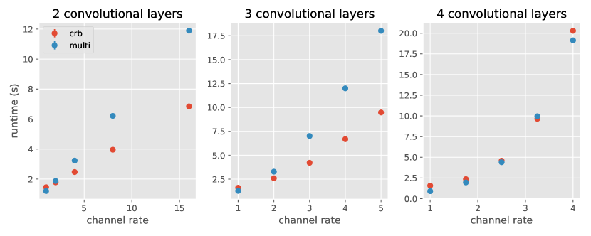
Figure 1: Runtime in seconds for processing 20 batches of 8 examples, in CNNs of increasing size. The channel rate is defined as the ratio between the number of channels from a layer to the previous, considering the first layer has 25 channels. Convolutions are performed with a kernel of size 3; ReLU activations are added after each convolution, and a max-pooling layer is added after every 2 convolutional layers. Inputs are randomly generated and have size $3\times 256\times 256$. Left, center and right show results for 2, 3 and 4 layers respectively. Each point is the average over 10 runs.

As explained above, the multi approach consists in vectorizing the naive approach by creating multiple copies of the same model and backpropagating through all batch samples in parallel. One could criticize this approach for using a very large amount of memory, as many copies need to be created. However, it turns out this can be done without a single copy of the original model: this can be done using only pointers to the original parameters, which uses as much memory as other methods.

That being said, it is not clear which strategy will perform better in terms of runtime. Due to how computations are optimized in the GPU, analyzing the computational complexity of each approach is not necessarily useful. We will thus run a series of experiments in order to perform this comparison empirically.

All the experiments in this section have been performed on n1-standard-8 instance on GCP, with a Nvidia P100 GPU. The image used is based on Ubuntu 18.04, and had Python 3.5.3 and PyTorch 1.1 installed.

4.1 Toy networks

In a first experiment, we create convolutional architectures with 2, 3 and 4 sequential convolutional layers such that the number of channels from a layer to the next increases according to a given ratio. In Fig. 1, we show that, for shallower networks, crb runs faster than multi as we increase this ratio. Increasing the number of layers, however, seems to be an advantage for multi. Finally, in a network with 4 layers, the two methods are competitive.

Depth and number of channels are not the only quantities that affect runtime. In another experiment, we study how the runtime changes with batch size. For larger batches, crb seems to be the method of choice. As shown in Fig.  2, both naive and multi lead to a runtime which is linear over batch size; crb, however, seems to be piecewise linear: as the batch size increases, the slope decreases. This behaviour is due, presumably, to the way crb is able to exploit the GPU, transforming the original computation into a series of new convolutions of different complexity.

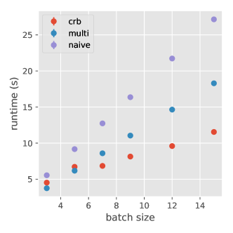
Figure 2: Runtime in seconds for processing 20 batches of different sizes, using the different strategies. Settings are similar to those of the previous experiment, except that i) the first layer now has 256 channels and ii) kernel size is set to 5, instead of 3. The channel rate is set to 1, and the number of layers to 3.

Other factors can come into play, and it is not always intuitive to understand which ones and why. For instance, increasing the kernel size of the convolutions seems to be an advantage for crb, see Fig. 3.

4.2 Realistic networks

At this point, one might wonder which of these approaches are better suited for calculating per-example gradients for practical DCNNs. Such DCNNs typically contain many more than 4 layers, as well as widely varying channel rates. To answer this question, we ran the same experiment for two popular DCNN architectures, AlexNet and VGG16. Runtime results are presented in Table 1.

Model	Batch Size	No DP (sec)	Naive (sec)	crb (sec)	multi (sec)
AlexNet	16	$0.747\pm 0.003$	$30.17\pm 0.02$	$2.030\pm 0.002$	$3.076\pm 0.005$
VGG16	8	$1.947\pm 0.001$	$37.20\pm 0.10$	$5.591\pm 0.006$	$4.630\pm 0.020$

Table 1: Runtime in seconds for processing 20 batches on AlexNet and VGG16. Inputs are randomly generated and have size $3\times 256\times 256$. For each model, we used a batch size that could reasonably fit into GPU memory. Implementations were taken from the torchvision library.

For relatively small networks such as AlexNet, crb performs up to fifteen times times faster than naive on a Nvidia P100 GPU. It is also slightly faster than multi. However, when looking at the larger VGG16, crb becomes slightly slower than multi. One could thus hypothesize that multi is the best option for larger networks; as noted before, however, it is not obvious whether width and depth are the only relevant quantities in play. Batch size, as well as the kernel size of the convolution, seem to be of relevance as well.

Notice that we have not used batch normalization layers in any of the networks, as they mix different examples on the batch and thus make per-gradient computations impossible. For this same reason we have not tested CNNs which naturally include batch normalization layers, such as the ResNet. An alternative is to use instance normalization in cases when per-example gradient clipping is necessary.

Our experiments show that both multi and crb methods have configurations in which they are the most efficient. Both methods have their merits while using similar amount of GPU memory.

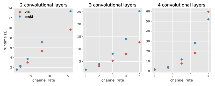
Figure 3: Analogous to Figure 1, except that kernel size of convolutions is set to 5 instead of 3. Increasing the kernel size seems to be an advantage to the crb strategy.

5 Conclusion

Both the existing multi approach and our extended crb are capable of fully utilizing GPU capabilities to efficiently compute per-example gradients. We have shown, empirically, that each is faster in a particular region of the parameter space of DCNN architectures. In general, it is unclear which method will be more efficient.

Our approach is more complicated to be put in practice: it requires one to adapt backpropagation hooks, as opposed to multi, for which multiple copies of the model can be created on a higher level. Notice also that our approach uses PyTorch’s peculiarities—namely the group argument in the convolutional layer—and should be adapted to different deep learning frameworks. Our hope is that the findings we present in this work will be useful in furthering the development and improvement of ML components necessary for privacy-aware machine learning.

We have implemented a PyTorch version extending torch.nn, which is available at https://github.com/owkin/grad-cnns.

References

- [1] Reza Shokri, Marco Stronati, Congzheng Song and Vitaly Shmatikov “Membership inference attacks against machine learning models” In 2017 IEEE Symposium on Security and Privacy (SP), 2017, pp. 3–18 IEEE
- [2] Nicholas Carlini et al. “The secret sharer: Measuring unintended neural network memorization & extracting secrets” In arXiv preprint arXiv:1802.08232, 2018
- [3] Luca Melis, Congzheng Song, Emiliano De Cristofaro and Vitaly Shmatikov “Exploiting unintended feature leakage in collaborative learning” In 2019 IEEE Symposium on Security and Privacy (SP), 2019, pp. 691–706 IEEE
- [4] Samuel Yeom, Irene Giacomelli, Matt Fredrikson and Somesh Jha “Privacy risk in machine learning: Analyzing the connection to overfitting” In 2018 IEEE 31st Computer Security Foundations Symposium (CSF), 2018, pp. 268–282 IEEE
- [5] Cynthia Dwork and Aaron Roth “The algorithmic foundations of differential privacy” In Foundations and Trends® in Theoretical Computer Science 9.3–4 Now Publishers, Inc., 2014, pp. 211–407
- [6] Martin Abadi et al. “Deep learning with differential privacy” In Proceedings of the 2016 ACM SIGSAC Conference on Computer and Communications Security, 2016, pp. 308–318 ACM
- [7] Ziyu Wang et al. “Dueling Network Architectures for Deep Reinforcement Learning” In International Conference on Machine Learning, 2016, pp. 1995–2003
- [8] Ian Goodfellow “Efficient per-example gradient computations” In arXiv preprint arXiv:1510.01799, 2015
- [9] Guillaume Alain et al. “Variance reduction in sgd by distributed importance sampling” In arXiv preprint arXiv:1511.06481, 2015
- [10] Abhishek Bhowmick et al. “Protection against reconstruction and its applications in private federated learning” In arXiv preprint arXiv:1812.00984, 2018