Non-Faradaic electric currents in the Nernst-Planck equations
and ‘action at a distance’ diffusiophoresis in crossed salt gradients

Abstract

In the Nernst-Planck equations in two or more dimensions, a non-Faradaic electric current can arise as a consequence of connecting patches with different liquid junction potentials. Whereas this current vanishes for binary electrolytes or one-dimensional problems, it is in general non-vanishing for example in crossed salt gradients. For a suspended colloidal particle, electrophoresis in the corresponding electrostatic potential gradient is generally vectorially misaligned with chemiphoresis in the concentration gradients, and diffusiophoresis (via electrophoresis) can occur in regions where there are no local concentration gradients (‘action at a distance’). These phenomena may provide new opportunities to manipulate and sort particles, in microfluidic devices for example.

The growing realisation that diffusiophoresis is a potent and ubiquitous non-equilibrium transport mechanism for micron-sized colloidal particles has led to a recent surge of interest in the phenomenon Abécassis et al. (2008); Palacci et al. (2012); Reinmüller et al. (2013); Florea et al. (2014); Shi et al. (2016); Banerjee et al. (2016); Keh (2016); Velegol et al. (2016); Shin et al. (2017a, b). For example, diffusiophoresis is effective at injecting or ousting particles from dead-end channels Kar et al. (2015); Shin et al. (2016), has been identified as a hitherto unsuspected pore-scale particulate soil removal process in laundry detergency Shin et al. (2018), implicated as a general non-motor transport mechanism in cells Sear (2019), and can be used to manipulate and sort particles by size and charge Shin et al. (2016, 2017c). The biggest effects arise in electrolyte solutions, where chemiphoresis in concentration gradients combines with electrophoresis in the diffusion potential to drive particles at speeds of 1–10 $\upmu\mathrm{m}\,\mathrm{s}^{-1}$ Anderson (1989), propelling them over large distances in time scales of minutes. An additional peculiarity in binary electrolytes is that the speed is logarithmically dependent on the concentration, leading to persistent effects such as osmotic trapping Palacci et al. (2012), and long-lived particle removal Shin et al. (2018).

To my knowledge, the existing phenomena that have been discussed in the above context pertain to binary electrolytes or assume one-dimensional gradients Brown and Poon (2014); Chiang and Velegol (2014); Shi et al. (2016); Gupta et al. (2019a, b). In this article, I argue that a still further enriched phenomenology arises in multicomponent electrolytes when concentration gradients are superimposed in different directions (‘crossed’ salt gradients). In part this is because chemiphoresis decouples partially from electrophoresis, but additionally it is because a non-vanishing electric current arises even in the absence of Faradaic reactions, when patches with different liquid junction potentials are connected by the intervening electrolyte solution. In itself this is surely a fascinating phenomenon, but importantly for diffusiophoresis, the presence of electric fields in bulk regions where there are no local concentration gradients implies that particles should move in those regions, as a kind of diffusiophoretic ‘action at a distance’. Since it seems quite easy to engineer crossed gradients either in microfluidics devices or with suitably chosen ‘soluto-inertial beacons’ as sources and sinks Banerjee et al. (2016); Banerjee and Squires (2019), these observations provide novel opportunities for particle manipulation and sorting.

Let me start with the Nernst-Planck equations which govern ion transport in these problems Levich (1962); Newman and Thomas-Alyea (2004),

$$\frac{\partial\rho_{i}}{\partial t}+\nabla\cdot\mathbf{J}_{i}=0\,,\quad\mathbf{J}_{i}=-D_{i}(\nabla\rho_{i}+\rho_{i}z_{i}\nabla\varphi)\,.$$ (1)

In these, $\rho_{i}$ is the density of the $i$-th ionic species, $D_{i}$ is the corresponding diffusion coefficient, $z_{i}$ the charge on the ion in units of $e$, where $e$ is the unit of elementary charge, and $\varphi=e\phi/k_{\mathrm{B}}T$ is a dimensionless electrostatic potential wherein $k_{\mathrm{B}}T$ is the unit of thermal energy and $\phi$ is the actual electrostatic potential. Eqs. (1) combine mass conservation laws for the individual ion densities with expressions for the fluxes driven by diffusion and drift in the electric field. For simplicity I omit advection terms although these are certainly relevant in microfluidics devices, and may additially arise if bulk flows are driven by diffusio-osmotic effects Shin et al. (2016).

The Nernst-Planck equations must be augmented by a closure for the electrostatic potential. At a fundamental level this is the Poisson equation, $\epsilon\nabla^{2}\phi=-e\rho_{z}$, where $\rho_{z}=\sum_{i}z_{i}\rho_{i}$ is the space charge (in units of $e$) and $\epsilon$ is the permittivity (assumed constant) of the supporting medium. The combined set are then known as the Poisson-Nernst-Planck (PNP) equations. Introducing the Debye length $\lambda_{\text{D}}=(\epsilon k_{\mathrm{B}}T/e^{2}\!\rho_{\text{D}})^{1/2}$, where $\rho_{\text{D}}=\sum_{i}z_{i}^{2}\rho_{i}$, allows the Poisson equation to be written as $\lambda_{\text{D}}^{2}\,\nabla^{2}\varphi=-{\rho_{z}}/{\rho_{\text{D}}}$. This makes it clear that if the problem size $L\gg\lambda_{\text{D}}$, the bare electrostatics problem is singular Hafemann (1965); Hickman (1970); Jackson (1974); Aguilella et al. (1987); Bazant et al. (2004); Janssen and Bier (2018), in the sense that there is an ‘outer’ domain on the length scale $O(L)$ in which $\rho_{z}\approx 0$ (local charge neutrality), asymptotically matched to ‘inner’ solutions on a length scale $O(\lambda_{\text{D}})$ (i. e. electric double layers or EDLs), whenever the boundary conditions would otherwise over-determine $\varphi$ in the outer domain edl .

Crucially, local charge neutrality does not necessarily imply a vanishing electric current $\mathbf{I}=\sum_{i}\,z_{i}\mathbf{J}_{i}$ (in units of $e$) in the outer domain. Rather, by summing the mass conservation laws in Eqs. (1) one can only conclude that the current should be solenoidal ($\nabla\cdot\mathbf{I}=0$). In fact, even for pure diffusion problems without Faradaic reactions dhu , a non-vanishing current ($\mathbf{I}\neq 0$) is not only possible but may be mandatory. To see this, insert the fluxes $\mathbf{J}_{i}$ from Eqs. (1) into the definition of $\mathbf{I}$ to obtain

$$\mathbf{I}=-\nabla g+\sigma\mathbf{E}\,.$$ (2)

This decomposes $\mathbf{I}$ into the sum of a diffusion current, and a conduction current obeying Ohm’s law Newman and Thomas-Alyea (2004). In this $g={\textstyle\sum_{i}}\,z_{i}D_{i}\rho_{i}$ is a weighted sum of ion densities, $\sigma={\textstyle\sum_{i}}\,z_{i}^{2}D_{i}\rho_{i}$ is the conductivity, and $\mathbf{E}=-\nabla\varphi$ is the electric field (the latter two are in semi-reduced units). Proceeding from Eq. (2), if $\mathbf{I}=0$ then it is easy to show $\nabla\times\mathbf{E}=\sigma^{-2}\,{\nabla\sigma\times\nabla g}$. But there is no particular reason why the cross product on the right hand side should vanish, even though $\nabla\times\mathbf{E}=0$ because $\mathbf{E}=-\nabla\varphi$. Thus we are forced to conclude that in general $\mathbf{I}\neq 0$. As another way to see this, by taking the curl of Eq. (2) one can eliminate the electrostatic potential to find

$$\sigma\,\nabla\times\mathbf{I}=\nabla\sigma\times(\mathbf{I}+\nabla g)\,.$$ (3)

This is an inhomogeneous partial differential equation for $\mathbf{I}$, and again supports the notion that $\mathbf{I}\neq 0$ is driven by crossed gradients in the form $\nabla\sigma\times\nabla g\neq 0$.

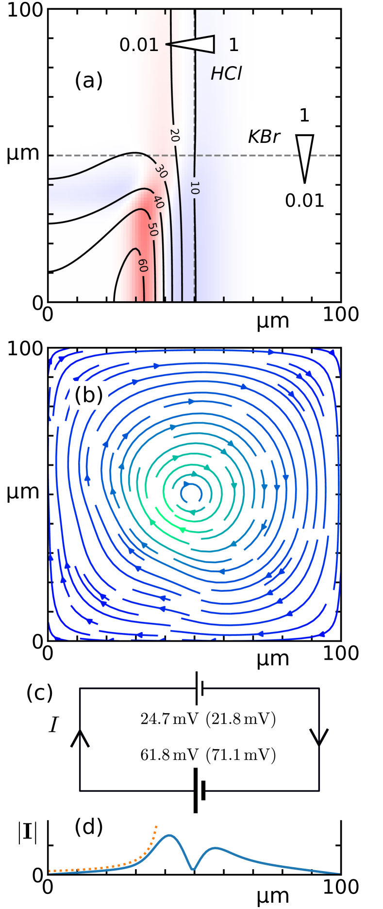
Figure 1: Crossed salt gradients at $t=0$, between HCl (horizontal) and KBr (vertical) sha : (a) electrostatic potential (equipotential lines labelled in $\mathrm{m\kern-0.50003pt{}V}$) and space charge (colored background); (b) circulating electric current (colored by magnitude); (c) equivalent circuit with HCl gradients labelled by liquid junction potentials (in brackets are the ‘open circuit’ values calculated from $\Delta\varphi=-\beta\ln(\sigma_{2}/\sigma_{1})$ where $\sigma_{2}/\sigma_{1}$ is the ratio of conductivities across the junction bin ); (d) magnitude of current along the $x=y$ diagonal (the dotted line is $1/r\sim 1/|x-x_{0}|$ where $x_{0}=40\,\upmu\mathrm{m}$).

Of course there are many examples where $\mathbf{I}$ does vanish. One such case is where the gradients are one-dimensional so that $\varphi$ can be found by quadrature Gupta et al. (2019a). Another important case is that of a binary electrolyte Levich (1962); Newman and Thomas-Alyea (2004) for which $\varphi=-\beta\ln\rho_{s}$ (the diffusion or liquid junction potential). Here $\beta={(D_{1}-D_{2})}{(q_{1}D_{1}+q_{2}D_{2})}$ is a normalised diffusivity contrast, and I suppose that $z_{1}>0$ and $z_{2}<0$, set $q_{i}=|z_{i}|$, and use $\rho_{s}=\rho_{1}/q_{2}=\rho_{2}/q_{1}$ for the overall electrolyte concentration bin .

The simplest situation where an electric current does arise is where there are three ion species, with crossed gradients. To explore this, suppose there are two cations with a common anion. Let the respective ion densities be $\rho_{1}$, $\rho_{2}$ and $\rho_{0}$, with corresponding diffusivities $D_{1}$, $D_{2}$ and $D_{0}$, and let the ions be univalent ($|z_{i}|=1$). For local charge neutrality we have $\rho_{0}=\rho_{1}+\rho_{2}$. Then $\nabla\sigma\times\nabla g=2D_{0}(D_{2}-D_{1})\nabla\rho_{1}\times\nabla\rho_{2}$. This suggests that the appearance of an electric current requires crossed gradients and contrasting cation diffusivities ($D_{1}\neq D_{2}$), but no particular requirement is placed on the anion diffusivity. Thus one of the gradients can be in a supporting electrolyte (i. e. $\beta\approx 0$), as in the example below.

To summarise the mathematical problem thus far, given $g$ and $\sigma$ and supposing that $\mathbf{I}\cdot\mathbf{n}$ is specified on the boundaries of the domain of interest, we must find the current distribution that satisfies Eq. (2) with $\nabla\cdot\mathbf{I}=0$ and $\mathbf{E}=-\nabla\varphi$. To prove solutions do exist, and are unique, we can note that this combination implies Newman and Thomas-Alyea (2004); Rica and Bazant (2010)

$$\nabla\cdot(\sigma\nabla\varphi)+\nabla^{2}\!g=0\,.$$ (4)

This is an inhomogeneous Poisson equation for $\varphi$ with the equivalent of a spatially-varying dielectric permittivity. Existence and uniqueness of $\varphi$ (up to an additive constant) then follows by analogy with standard electrostatics Coulson (1961). A direct proof is also given in Appendix A. Eq. (4) is non-singular and amenable to solution by standard numerical methods Press et al. (2007), and replaces the original electrostatic Poisson equation in closing the Nernst-Planck equations. Additionally, I show in Appendix B that the variational principle equivalent to Eq. (4) corresponds to minimising the total Ohmic heating $\int\mathbf{I}^{2}/2\sigma\,{\mathrm{d}}V$ modulo a surface term. Recalling that the problem is athermal, this can be interpreted as a proxy minimum entropy production principle. The connection to the true entropy production in the underlying PNP equations is left for future work.

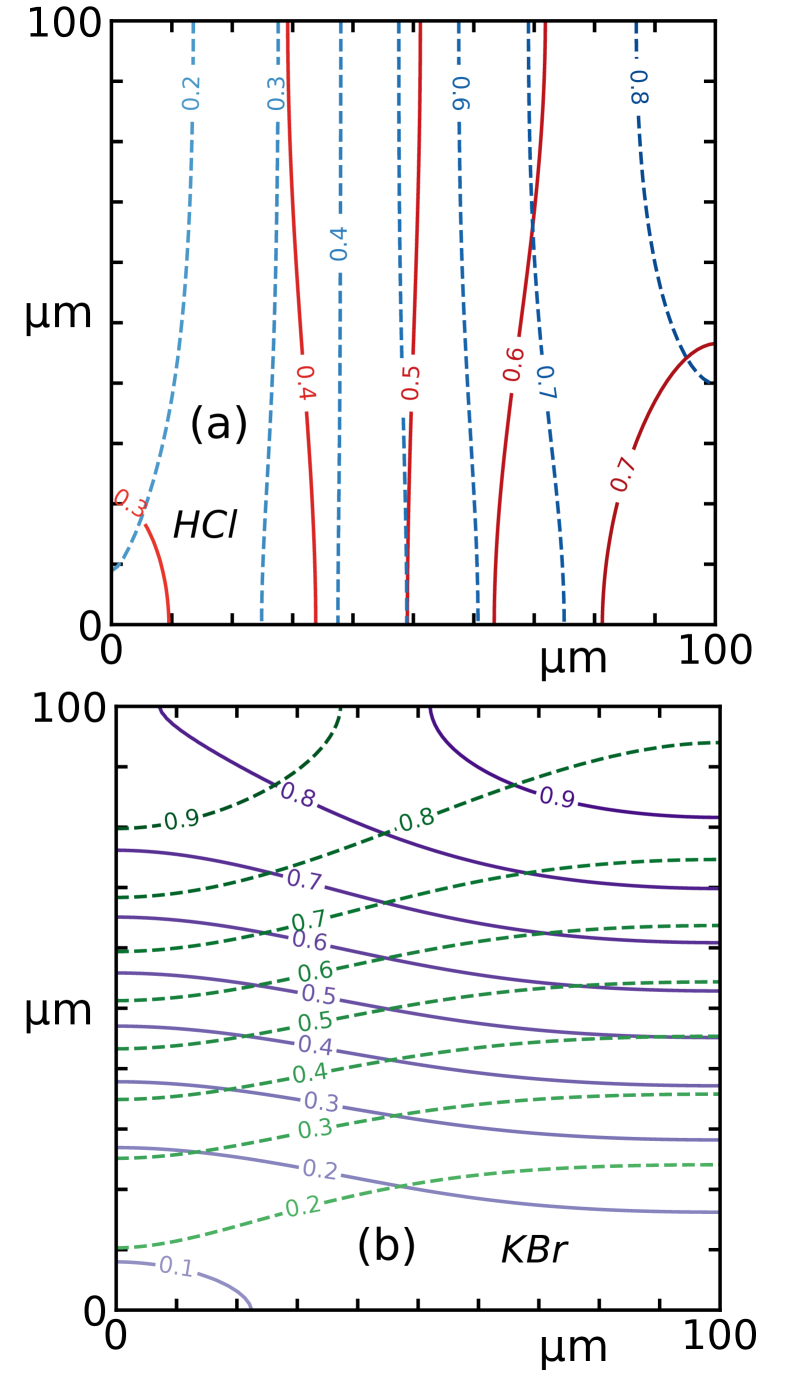
Figure 2: Ion density profiles at $t=250\,\mathrm{ms}$, for (a) HCl and (b) KBr. Contours are shown as solid and dashed lines for cations and anions respectively, labelled by concentration using the same scale as Fig. 1a.

Let me turn now to a specific numerical example which demonstrates the principles by which a non-vanishing electric current arises. For concreteness I consider an enclosed square domain of side 100 $\upmu\mathrm{m}$, initialised at $t=0$ with a 100-fold gradient in an electrolyte with a large diffusivity contrast (HCl, $\beta=0.64$), crossed with a 100-fold gradient in a supporting electrolyte (KBr, $\beta=-0.01$) dif . The concentration gradients are initially localised to the mid-planes, with widths $10\,\upmu\mathrm{m}$ sha , so that the square domain is divided into four quadrants as shown in Fig. 1a. The actual concentration units need not be specified since the overall units of concentration can be factored out of the Nernst-Planck equations. For this demonstration I choose a problem with four rather than three ions, since this maintains the distinction between the two electrolytes.

I solve Eq. (4) in this square domain, with $\mathbf{I}\cdot\mathbf{n}=0$ on the boundaries. For details see Appendix C. Fig. 1a shows that there is a significant liquid junction potential ($\Delta\phi\approx 62\,\mathrm{m\kern-0.50003pt{}V}$) between the two lower quadrants, corresponding approximately to the expected value for HCl treated as a binary electrolyte. The junction potential between the upper two quadrants is much weaker though ($\Delta\phi\approx 25\,\mathrm{m\kern-0.50003pt{}V}$), as might be expected for HCl in the presence of a supporting electrolyte bin . It is essentially this difference that drives the circulating electric current (Fig. 1b). By joining the upper and lower halves, it is as if we have short-circuited the two liquid junctions, as sketched in Fig. 1c. The resulting current is distributed throughout the square domain, as befits the minimum Ohmic heating principle. Crucially, in the lower-left quadrant where the conductivity is small, this generates a significant electric field throughout this region as indicated by the equipotential lines in Fig. 1a. Also shown in Fig. 1a is the space charge from $\rho_{z}=-(\epsilon k_{\mathrm{B}}T/e^{2})\,\nabla^{2}\varphi$. Note that $|\rho_{z}|\lesssim 10^{-8}\,\mathrm{M}$ so that local charge neutrality should normally be a very good approximation rho . Finally, Eq. (3) implies $\mathbf{I}$ should be irrotational as well as solenoidal, in regions where the gradients vanish. This explains why approximately $|\mathbf{I}|\sim 1/r$ in the lower left quadrant (Fig. 1d), and why the equipotential lines are approximately radial in this quadrant (Fig. 1a).

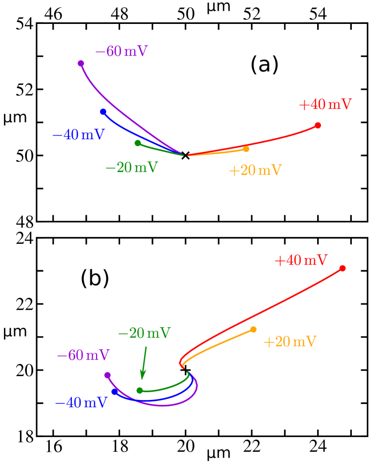
Figure 3: Diffusiophoresis: trajectories of colloid particles with different zeta potentials (labels) starting from (a) the centre of the crossed gradients, and (b) a location in the lower left quadrant. Starting points are marked by a cross, and positions at $t=500\,\mathrm{ms}$ by filled circles.

As time progresses, the gradients in this confined system dissipate by coupled diffusion. To track the evolving concentration fields, I solve the Nernst-Planck equations with boundary conditions $\mathbf{J}_{i}\cdot\mathbf{n}=0$, computing the electrostatic potential from Eq. (4) at each step tim . Fig. 2 shows the situation after 250 ms. In the upper half space the more mobile $\mathrm{H}^{+}$ has spread out much further than the less mobile $\mathrm{Cl}^{-}$ (Fig. 2a), since with the high concentration of KBr in this region the ion densities become decoupled. Additionally the circulating current corresponds to cations moving clockwise and anions moving anticlockwise, which distorts the ion density profiles, as seen for $\mathrm{K}^{+}$ and $\mathrm{Br}^{-}$ (Fig. 2b).

What are the implications for diffusiophoresis of a suspended colloidal particle? Obviously, this depends on where the particle is located as well as its zeta potential. Here I predict trajectories by integrating ${\mathrm{d}}\mathbf{R}/{\mathrm{d}}t=\mathbf{U}$, where the diffusiophoretic drift velocity is Anderson (1989); Shi et al. (2016); Gupta et al. (2019b); uni

$$\mathbf{U}=\frac{\epsilon}{\eta}\,\Bigl{(}\frac{k_{\mathrm{B}}T}{e}\Bigr{)}^{2}\Bigl{[}4\ln\cosh\Bigl{(}\frac{{\overline{\zeta}}}{4}\Bigr{)}\,\nabla\ln\rho-{\overline{\zeta}}\,\nabla\varphi\Bigr{]}$$ (5)

(see also Appendix D). In this $\rho=\sum_{i}\rho_{i}$ is the total ion density, $\eta$ is the viscosity of the medium, and ${\overline{\zeta}}=e\zeta/k_{\mathrm{B}}T$ is the non-dimensionalised zeta potential. The two terms in Eq. (5) correspond respectively to chemiphoresis in the overall concentration gradient, and electrophoresis in the electrostatic potential gradient.

Sample trajectories are shown in Fig. 3. In the lower-left quadrant (Fig. 3b) the electric field corresponding to the gradient in $\phi$ drives diffusiophoresis via electrophoresis even though there are initially no local concentration gradients. I term this unusual phenomenon diffusiophoretic ‘action at a distance’. Since the electric field also drives the electric current, in this quadrant $\mathbf{U}$ is initally parallel to $\mathbf{I}$; this explains the initial coincidence of the trajectories. In contrast, for a particle which finds itself in the middle of the crossed salt gradients (Fig. 3a), electrophoresis and chemiphoresis are vectorially misaligned even initially, so that particles with different zeta potentials are propelled along diverging trajectories even if they have the same sign of charge.

The design of devices which exploit these striking effects is a clearly a promising avenue for future work. I note that in this situation one loses the logarithmic sensitivity exhibited in binary electrolytes Palacci et al. (2012); Shin et al. (2018); log , so that the distance over which particles move is limited by the relaxation time for the ion densities. This can be alleviated by using soluto-inertial beacons Banerjee et al. (2016); Banerjee and Squires (2019), or microfluidic devices in which long-lived gradients can be established Abécassis et al. (2008); Shi et al. (2016); Shin et al. (2017a).

To summarise, a rich phenomenology arises in the Nernst-Planck equations when considering multicomponent electrolytes in more than one dimension. In particular, circulating (solenoidal) electric currents appear when patches with different liquid junction potentials are connected by the intervening electrolyte solution. The electric fields associated with these currents can drive ‘action at a distance’ diffusiophoresis of suspended colloidal particles, even in the absence of local concentration gradients. This is a definitive prediction of the Nernst-Planck equations, combined with the current understanding of diffusiophoresis of charged colloidal particles, and it would be fascinating to put to an experimental test.

Appendix A Uniqueness

Here I provide a direct proof of uniqueness of $\varphi$ in Eq. (4). Suppose there are two solution pairs $(\mathbf{I}_{1},\varphi_{1})$ and $(\mathbf{I}_{2},\varphi_{2})$, such that $\mathbf{I}_{1}\cdot\mathbf{n}=\mathbf{I}_{2}\cdot\mathbf{n}$ on some domain boundary with vector normal $\mathbf{n}$. Subtracting the corresponding versions of Eq. (2) yields a homogeneous problem in which the difference solution, with $\mathbf{I}=\mathbf{I}_{2}-\mathbf{I}_{1}$ and $\varphi=\varphi_{2}-\varphi_{1}$, satisfies Ohm’s law $\mathbf{I}=\sigma\mathbf{E}$ where $\mathbf{I}\cdot\mathbf{n}=0$ on the domain boundary, $\nabla\cdot\mathbf{I}=0$ in the interior, and $\mathbf{E}=-\nabla\varphi$. Now consider

$$\nabla\cdot(\varphi\mathbf{I})=\varphi\,(\nabla\cdot\mathbf{I})+\mathbf{I}\cdot\nabla\varphi\,.$$ (6)

The first term on the right hand side vanishes as a consequence of the solenoidal nature of $\mathbf{I}$, and the second term simplifies to $\mathbf{I}\cdot\nabla\varphi=-\sigma\mathbf{E}^{2}$. Integrate Eq. (6) over the domain of interest and use the divergence theorem to get

$${\textstyle\int}\nabla\cdot(\varphi\mathbf{I})\,{\mathrm{d}}V={\textstyle\int}\varphi\mathbf{I}\cdot\mathbf{n}\,{\mathrm{d}}S=0$$ (7)

(because $\mathbf{I}\cdot\mathbf{n}=0$ on the boundary). We conclude that

$${\textstyle\int}\sigma\mathbf{E}^{2}\,{\mathrm{d}}V=0\,.$$ (8)

But $\sigma>0$ and $\mathbf{E}^{2}\geq 0$, so this implies $\mathbf{E}=0$ everywhere, and hence $\mathbf{I}=0$ and $\varphi=\mathrm{constant}$. This is the desired result. It means that the solution pairs $(\mathbf{I}_{1},\varphi_{1})$ and $(\mathbf{I}_{2},\varphi_{2})$ in the original inhomogeneous problem can at most differ by a constant in $\varphi$.

Appendix B Variational principle

An inhomogeneous Poisson equation such as that given in Eq. (4) has an equivalent variational principle. In the present case it is

$$\frac{\delta}{\delta\varphi(\mathbf{r})}\Bigl{[}{\textstyle\int}({\textstyle\frac{1}{2}}\sigma|\nabla\varphi|^{2}-\varphi\nabla^{2}g)\,{\mathrm{d}}V\Bigr{]}=0\,.$$ (9)

Making use of the vector calculus identity

$$\nabla\cdot(\varphi\nabla g)=\nabla\varphi\cdot\nabla g+\varphi\nabla^{2}g\,,$$ (10)

the integrand in the above can be reformulated to

$$\begin{split}&{\textstyle\frac{1}{2}}{\sigma|\nabla\varphi|^{2}}-\varphi\nabla^{2}g\\[3.0pt] &\qquad{}=\frac{|\sigma\nabla\varphi+\nabla g|^{2}}{2\sigma}-\frac{|\nabla g|^{2}}{2\sigma}-\nabla\cdot(\varphi\nabla g)\,.\end{split}$$ (11)

The second term on the right hand side is constant, given $g$ and $\sigma$, and can be discarded. The third term can be replaced by a surface integral. Rewriting in terms of the currents, the variational principle can be rebranded as

$$\frac{\delta}{\delta\varphi(\mathbf{r})}\Bigl{[}{\textstyle\int}({\mathbf{I}^{2}}/{2\sigma})\,{\mathrm{d}}V-{\textstyle\int}\!\varphi\,\nabla g\cdot\mathbf{n}\,{\mathrm{d}}S\Bigr{]}=0\,.$$ (12)

Thus the electrostatic potential in Eq. (4) is such as to minimise the Ohmic heating (i. e. defined using the total current), modulo a surface term.

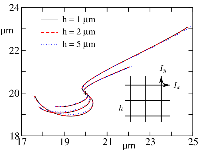
Figure 4: Dependence of trajectories in Fig. 3b on grid spacing.

Appendix C Numerical scheme

To solve the inhomogeneous Poisson equation, Eq. (4), I discretise the problem domain into a square grid of spacing $h$ (Fig. 4 inset). The potential $\varphi$ and the ion densities $\rho_{i}$ are defined on the nodes of the grid, and the fluxes $\mathbf{J}_{i}$ and current $\mathbf{I}$ are defined on the edges joining the nodes (shown in Fig. 4 inset for $I_{x}$ and $I_{y}$ components). With these definitions, $\nabla\cdot\mathbf{I}=0$ becomes the constraint that the sum of the currents entering each node should vanish. The number of constraints then matches the number unknowns (values of $\phi$ on the nodes) and the problem is linear, so in principle can be solved by any (sparse) linear algebra method. In practice I use a straightforward Gauss-Seidel iterative scheme that requires minimal bookkeeping, with the convergence criterion being that the relative change in $\varphi$ in subsequent iteractions falls to less than $10^{-14}$. For boundary conditions I set the fluxes to zero on the exterior edges. Note that the actual space charge is not represented as such in the calculation, and deviations from $\nabla\cdot\mathbf{I}=0$ are numerical errors.

To solve the time-dependent Nernst-Planck equations, I use a standard forward-time centered-space (FTCS) scheme Press et al. (2007) based on the above grid decomposition, with a time step $\delta t=0.025\,\mathrm{ms}\times(h/\upmu\mathrm{m})^{2}$, which comfortably satisfies the usual Courant-Friedrichs-Lewy condition since the maximum diffusion coefficient is $D=9.31\,\upmu\mathrm{m}^{2}\,\mathrm{ms}^{-1}$ (for $\mathrm{H}^{+}$) so $D\,\delta t/h^{2}<0.5$.

To compute the trajectories of particles undergoing diffusiophoresis I integrate the kinematic equations in Eq. (5) using a simple first order forward Euler scheme with $\Delta t=5\,\mathrm{ms}$ (a multiple of $\delta t$), and bivariate spline interpolation (on the same grid as above) to calculate off-lattice approximations to $\nabla\ln\rho$ and $\nabla\varphi$.

Fig. 4 shows that the computed trajectories depend very little on the underlying grid spacing and consequent choices for time step. I only show the $h$-dependence for trajectories of particles starting in the lower left quadrant; the trajectories of particles which start in the centre of the crossed gradients show even smaller $h$-dependence. All calculations reported in the main text are for $h=1\,\upmu\mathrm{m}$ (100² grid).

Appendix D Diffusiophoretic drift coefficients

Diffusiophoresis in multicomponent electrolytes has been considered by several groups recently Chiang and Velegol (2014); Shi et al. (2016); Gupta et al. (2019b). Assuming a thin EDL, it is convenient to start with a general expression for the diffusiophoretic drift of a suspended colloidal particle arising from bulk chemical potential gradients,

$$\mathbf{U}={\textstyle\sum_{i}}{\mathcal{M}}_{i}\nabla\mu_{i}\,.$$ (13)

Restricting the analysis to the tractable but practically relevant case of monovalent electrolytes, the mobilities are ${\mathcal{M}}_{i}=(\rho_{i}/\rho)\times{\mathcal{M}}_{\pm}$ where Shi et al. (2016)

$${\mathcal{M}}_{\pm}=\frac{\epsilon k_{\mathrm{B}}T}{\eta e^{2}}\Bigr{[}4\ln\cosh\frac{e\zeta}{4k_{\mathrm{B}}T}\mp\frac{e\zeta}{k_{\mathrm{B}}T}\Bigr{]}$$ (14)

according to the sign of the ion ($z_{i}=\pm 1$). Here $\rho=\sum_{i}\rho_{i}$ as in the main text, $\eta$ is viscosity, and $\zeta$ is the particle zeta potential. This formalism extends to include electrophoresis if one employs the electrochemical potentials,

$$\mu_{i}=k_{\mathrm{B}}T\ln\rho_{i}+ez_{i}\phi\,.$$ (15)

Combining Eqs. (13) and (14), cross terms cancel since $\sum_{i}z_{i}\rho_{i}=0$, yielding Eq. (5) used in the main text. Note that the second term in Eq. (5) simplifies to the well-known Helmholtz-Smoluchowski result $-(\epsilon\zeta/\eta)\nabla\phi$ Anderson (1989).

References

- Abécassis et al. (2008) B. Abécassis, C. Cottin-Bizonne, C. Ybert, A. Ajdari, and L. Bocquet, Nat. Mater. 7, 785 (2008).
- Palacci et al. (2012) J. Palacci, C. Cottin-Bizonne, C. Ybert, and L. Bocquet, Soft Matter 8, 980 (2012).
- Reinmüller et al. (2013) A. Reinmüller, H. J. Schöpe, and T. Palberg, Langmuir 29, 1738 (2013).
- Florea et al. (2014) D. Florea, S. Musa, J. M. Huyghe, and H. M. Wyss, Proc. Natl. Acad. Sci. USA 111, 6554 (2014).
- Shi et al. (2016) N. Shi, R. Nery-Azevedo, A. I. Abdel-Fattah, and T. M. Squires, Phys. Rev. Lett. 117, 258001 (2016).
- Banerjee et al. (2016) A. Banerjee, I. Williams, R. N. Azevedo, M. E. Helgeson, and T. M. Squires, Proc. Natl. Acad. Sci. USA 113, 8612 (2016).
- Keh (2016) H. J. Keh, Curr. Opin. Colloid In. 24, 13 (2016).
- Velegol et al. (2016) D. Velegol, A. Garg, R. Guha, A. Kara, and M. Kumara, Soft Matter 12, 4686 (2016).
- Shin et al. (2017a) S. Shin, O. Shardt, P. B. Warren, and H. A. Stone, Nat. Commun. 8, 15181 (2017a).
- Shin et al. (2017b) S. Shin, J. T. Ault, P. B. Warren, and H. A. Stone, Phys. Rev. X 7, 041038 (2017b).
- Kar et al. (2015) A. Kar, T.-Y. Chiang, I. O. Rivera, A. Sen, and D. Velegol, ACS Nano 9, 746 (2015).
- Shin et al. (2016) S. Shin, E. Um, B. Sabass, J. T. Ault, M. Rahimi, P. B. Warren, and H. A. Stone, Proc. Natl. Acad. Sci. USA 113, 257 (2016).
- Shin et al. (2018) S. Shin, P. B. Warren, and H. A. Stone, Phys. Rev. Appl. 9, 034012 (2018).
- Sear (2019) R. P. Sear, Phys. Rev. Lett. 122, 128101 (2019).
- Shin et al. (2017c) S. Shin, J. T. Ault, J. Feng, P. B. Warren, and H. A. Stone, Adv. Mater. 29, 1701516 (2017c).
- Anderson (1989) J. L. Anderson, Ann. Rev. Fluid Mech. 21, 61 (1989).
- Brown and Poon (2014) A. Brown and W. Poon, Soft Matter 10, 4016 (2014).
- Chiang and Velegol (2014) T.-Y. Chiang and D. Velegol, J. Colloid Interf. Sci. 424, 120 (2014).
- Gupta et al. (2019a) A. Gupta, S. Shim, L. Issah, C. McKenzie, and H. A. Stone, Soft Matter (2019a), 10.1039/C9SM01780A.
- Gupta et al. (2019b) A. Gupta, B. Rallabandi, and H. A. Stone, Phys. Rev. Fluids 4, 043702 (2019b).
- Banerjee and Squires (2019) A. Banerjee and T. M. Squires, Sci. Adv. 5, eaax1893 (2019).
- Levich (1962) V. G. Levich, Physicochemical Hydrodynamics (Prentice-Hall, Englewood Cliffs, NJ, 1962).
- Newman and Thomas-Alyea (2004) J. Newman and K. E. Thomas-Alyea, Electrochemical Systems (John Wiley & Sons, Hoboken, NJ, 2004).
- Hafemann (1965) D. R. Hafemann, J. Phys. Chem. 69, 4226 (1965).
- Hickman (1970) H. J. Hickman, Chem. Eng. Sci. 25, 381 (1970).
- Jackson (1974) J. L. Jackson, J. Phys. Chem. 78, 2060 (1974).
- Aguilella et al. (1987) V. M. Aguilella, S. Mafé, and J. Pellicer, Electrochim. Acta 32, 483 (1987).
- Bazant et al. (2004) M. Z. Bazant, K. Thornton, and A. Ajdari, Phys. Rev. E 70, 021506 (2004).
- Janssen and Bier (2018) M. Janssen and M. Bier, Phys. Rev. E 97, 052616 (2018).
- (30) The value of where the outer solution meets the EDLs cannot be pre-determined, and indeed it is the mismatch between this and the true wall boundary condition that gives rise to an EDL in the first place.
- (31) Technically I also assume small Dhukin number so that surface conduction in the EDLs can be neglected Anderson (1989).
- (32) The specific functional form is where and are the limiting concentrations in arbitrary units, is the distance from the mid-plane, and is the width.
- (33) The binary electrolye case can be solved because the individual ion densities are slaved to each other by local charge neutrality so that and . Hence and can be integrated to determine up to a a constant. A binary electrolyte with a uniform background can also be solved, since in that case also and therefore . This demonstrates that a background electrolyte reduces the diffusion potential, since it reduces the conductivity contrast; however the specific situation is transient since the electrostatic coupling in the Nernst-Planck equations will soon lead to all ion densities becoming non-uniform.
- Rica and Bazant (2010) R. A. Rica and M. Z. Bazant, Phys. Fluids 22, 112109 (2010).
- Coulson (1961) C. A. Coulson, Electricity (Oliver and Boyd, Edinburgh, 1961).
- Press et al. (2007) W. H. Press, S. A. Teukolsky, W. T. Vetterling, and B. P. Flannery, Numerical Recipes, 3rd ed. (CUP, New York, 2007).
- (37) The diffusivities of H+, Cl-, K+, and Br- are 9.31, 2.03, 1.96, and respectively, taken from a database in the PHREEQC software package; see D. L. Parkhurst and C. A. J. Appelo, Description of input and examples for PHREEQC version 3: a computer program for speciation, batch-reaction, one-dimensional transport, and inverse geochemical calculations, Tech. Rep. (U.S. Geol. Survey, Reston, VA, 2013). .
- (38) Interestingly the choice of units for the ion densities does not affect the calculation of the space charge .
- (39) The ion densities relax on a time scale since and . On the other hand, the time scale for the electrostatic potential and electric current to relax is Hickman (1970); Jackson (1974) (as an circuit, the relevant capacitance is smaller than in the EDL charging problem Bazant et al. (2004); Janssen and Bier (2018)). Then implies and are slaved to the ion densities. Further investigation of this aspect is left to future work.
- (40) Eq. (5) assumes the ions are univalent Gupta et al. (2019b).
- (41) Logarithmic sensitivity in binary electrolytes follows by inserting and into Eq. (5), whereupon both terms acquire the same dependence on .