Dynamic Structure of Hadrons in ChPT

Abstract

The Chiral Perturbation Theory (ChPT) has been very successful in describing low-energy hadronic properties in the non-perturbative regime of Quantum Chromodynamics. The results of ChPT, many of which are currently under active experimental investigation, provide stringent predictions of many fundamental properties of hadrons, including quantities such as electromagnetic polarizabilities. The paper outlines our semi-automated calculations in ChPT, the corresponding results for the electric and magnetic polarizabilities of the proton and our predictions for Compton differential cross sections.

I Formalism and Results

In general, polarizabilities are related to the deformability and stiffness of hadrons and can be experimentally accessed through Compton scattering. For the proton and neutron, electric ($\alpha$) polarizabilities are approximately the same, while magnetic ($\beta$) polarizabilities are different but both positive, which points to the paramagnetic nature of the nucleon. Although small (on order of $10^{-4}\,fm^{3}$), electric and magnetic polarizabilities were measured by several experimental groups. We can relate an amplitude to the set of Compton structure functions $R_{i}$ Babusci in the following way:

$$\frac{1}{8\pi W}M(\gamma B\rightarrow\gamma^{\prime}B)= R_{1}({\bf\epsilon}^{\prime*}\cdot{\bf\epsilon})+R_{2}({\bf s}{}^{\prime*}\cdot{\bf s})+iR_{3}{\bf\sigma}\cdot({\bf\epsilon}{}^{\prime*}\times{\bf\epsilon})+iR_{4}l{\bf\sigma}\cdot({\bf s}{}^{\prime*}\times{\bf s})$$ (1)

$$+iR_{5}(({\bf\sigma}\cdot\hat{{\bf k}})({\bf s^{\prime*}}\cdot{\bf\epsilon})-({\bf\sigma}\cdot\hat{{\bf k}}^{\prime})({\bf s}\cdot{\bf\epsilon^{\prime*}}))+iR_{6}(({\bf\sigma}\cdot\hat{{\bf k}}^{\prime})({\bf{\bf s^{\prime*}}}\cdot{\bf\epsilon})-({\bf\sigma}\cdot\hat{{\bf k}})({\bf s}\cdot{\bf\epsilon^{\prime*}})).$$

Here, $W=\omega+\sqrt{\omega^{2}+m_{B}^{2}}$ is the center of mass energy and $\omega$ is the energy of the incoming photon. Unit magnetic vector (${\bf s}=(\hat{{\bf k}}\times{\bf\epsilon}$)), polarization vector ($\boldsymbol{\epsilon}$) and unit momentum of the photon $\big{(}\hat{{\bf k}}={\bf k}/k\big{)}$ are denoted by the prime for the case of the outgoing photon. In our case we have computed the Compton scattering amplitude using CHM CHM in the basis of Dirac chains:

$$\frac{1}{8\pi W}M(\gamma B\rightarrow\gamma^{\prime}B)= f_{1}(\epsilon^{\prime*}k)\left[\overline{u}\left(p^{\prime}\right)\not{\epsilon}u\left(p\right)\right]+f_{2}(\epsilon k^{\prime})\left[\overline{u}\left(p^{\prime}\right)\not{\epsilon}^{\prime*}u\left(p\right)\right]+f_{3}(\epsilon^{\prime*}k)\left[\overline{u}\left(p^{\prime}\right)\not{\epsilon}\not{k}u\left(p\right)\right]$$

$$+f_{4}(\epsilon k^{\prime})\left[\overline{u}\left(p^{\prime}\right)\not{\epsilon}^{\prime*}\not{k}u\left(p\right)\right]+f_{5}\left[\overline{u}\left(p^{\prime}\right)\not{\epsilon}\not{\epsilon}^{\prime*}u\left(p\right)\right]+f_{6}(\epsilon\epsilon^{\prime*})\left[\overline{u}\left(p^{\prime}\right)u\left(p\right)\right]$$

$$+f_{7}(\epsilon k^{\prime})(\epsilon^{\prime*}k)\left[\overline{u}\left(p^{\prime}\right)u\left(p\right)\right]+f_{8}(\epsilon\epsilon^{\prime*})\left[\overline{u}\left(p^{\prime}\right)\not{k}u\left(p\right)\right]+f_{9}\left[\overline{u}\left(p^{\prime}\right)\not{\epsilon}\not{\epsilon}^{\prime*}\not{k}u\left(p\right)\right].$$ (2)

In this case we get nine Compton structure functions $f_{i}$. Here, all the dot products are defined in the four-dimensional space-time with the following metric $\left(1,-1,-1,-1\right)$, and $u(p)$ denotes the Dirac spinor for free baryon. The choice of the basis is not unique and can be defined differently (Babusci ), although the evaluation of the polarizabilities based on the basis in Eq.(1) is more convenient. Here, the structure functions $R_{i}$ are directly related to the electric, magnetic and spin-dependent polarizabilities in the multi-pole expansion. This includes loops (up to the given order of perturbation) and structure-dependent pole contributions, such as tree-level baryon resonance excitations and Wess-Zumino-Witten (WZW) (WZ , W ) anomalous interaction. Keeping only the dipole-dipole and dipole-quadrupole transitions in the multipole expansion of the Compton structure functions multi-1 ; multi-2 ; multi-3 , we connect the non-Born (NB) structure functions to the polarizabilities of the baryon in these simple equations:

$${\displaystyle R_{1}^{NB}=} \omega^{2}\alpha_{E1};\ \ R_{2}^{NB}=\omega^{2}\beta_{M1};\ \ R_{3}^{NB}=\omega^{3}(-\gamma_{E1E1}+\gamma_{E1M2});$$

$${\displaystyle R_{4}^{NB}=} \omega^{3}(-\gamma_{M1M1}+\gamma_{M1E2});\ \ R_{5}^{NB}=-\omega^{3}\gamma_{M1E2};\ \ R_{5}^{NB}=-\omega^{3}\gamma_{E1M2}.$$

Connecting Compton structure functions $f_{i}$ from Eq.2 to $R_{i}$ from Eq.1, we have:

$$R_{1}= {\displaystyle-\eta^{2}\chi m^{2}\left(f_{1}+f_{2}+f_{3}m(1+\eta+v)\left(1+\frac{\eta}{1+v}\right)\right)}-f_{5}m\left(1+v-\frac{2\eta^{2}\chi}{1+v}\right)-f_{6}m\left(1+v-\frac{\eta^{2}\chi}{1+v}\right)$$

$$+f_{7}\eta^{2}m^{3}\chi\left(1+v-\frac{\eta^{2}\chi}{1+v}\right)-f_{8}m^{2}\eta(1+v)\left(1+\frac{\eta(1+\chi)}{1+v}+\frac{\eta^{2}\chi}{(1+v)^{2}}\right)$$

$$-f_{9}\eta m^{2}\left(1+v+\eta+2\eta\chi\left(1+\frac{\eta}{1+v}\right)\right),$$

$$R_{2}= \eta^{2}m^{2}\left(f_{1}+f_{2}+f_{3}m(1+v+\eta)\left(1+\frac{\eta}{1+v}\right)\right)-f_{5}\frac{\eta^{2}m}{1+v}$$

$$-f_{7}\eta^{2}m^{3}\left(1+v-\frac{\eta^{2}\chi}{1+v}\right)+f_{9}\eta^{2}m^{2}\left(1+\frac{\eta}{1+v}\right),$$

$$R_{3}= 2\eta^{2}m^{2}\left(f_{1}-f_{3}m(1+v+\eta)-\chi\left(f_{2}+f_{3}m(1+v+\eta)\right)\right)+f_{5}m\left(1+v+\frac{2\eta^{2}\chi}{1+v}\right)+\frac{f_{6}\eta^{2}m\chi}{1+v}$$

$$-f_{7}\frac{\eta^{4}m^{3}\left(\chi^{2}-1\right)}{1+v}-f_{8}\eta^{2}m^{2}\chi\left(1+\frac{\eta}{1+v}\right)+f_{9}\eta m^{2}\left(1+v+\eta-2\eta\chi\left(1+\frac{\eta}{1+v}\right)\right),$$

$$R_{4}= \left(f_{5}+f_{6}\right)\frac{\eta^{2}m}{1+v}-\eta^{2}m^{2}\left(f_{8}+f_{9}\right)\left(1+\frac{\eta}{1+v}\right),$$

$$R_{5}= \eta^{2}m^{2}\left(f_{2}+f_{3}m(1+v+\eta)\right)-\left(f_{6}+2f_{5}\right)\frac{\eta^{2}m}{1+v}+f_{7}\frac{\eta^{4}m^{3}\chi}{1+v}+\eta^{2}m^{2}\left(f_{8}+2f_{9}\right)\left(1+\frac{\eta}{1+v}\right),$$

$$R_{6}= -\eta^{2}m^{2}\left(f_{1}-f_{3}m(1+v+\eta)\right)-f_{7}\frac{\eta^{4}m^{3}}{1+v},$$

where $\chi=\cos\theta_{c.m.}$, $\theta_{c.m.}$ is a photon scattering angle in the c.m.s. reference frame, $\eta=\frac{\omega}{m}$, and $v=\frac{E}{m}$, where $E$ is the energy of baryon in c.m.s. As one can see from Fig.1, the proton polarizabilities have almost no energy dependence below 50 MeV.

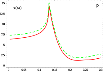
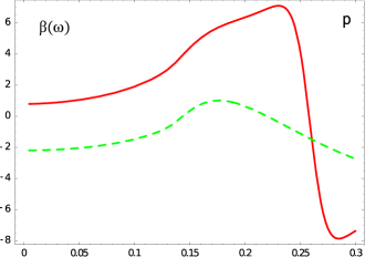
Figure 1: Dependencies of the proton electric and magnetic polarizabilities (in $10^{-4}\,(fm^{3})$) on photon energy $\omega$ (GeV) in c.m.s. The green-dashed curves correspond to the $\mathcal{O}\left(p^{3}\right)-\pi N$ loops contribution and WZW-anomaly. The solid-red curves include all the previous contributions plus the $\Delta$-pole resonance.

The electric proton polarizability has strong, resonance-type dependence near the pion production threshold. Of course, we need to add contribution from the resonances in the loops of Compton scattering. Hence, we have borrowed the resonance loops results from the small-scale expansion (SSE) approach (SSE ). If no $\Delta$-pole contribution is added, the magnetic polarizability in Fig.1 stays negative (diamagnetic) for almost all the energies. The $\Delta$-pole contribution is large enough to shift $\beta_{p}(\omega)$ from negative to positive (paramagnetic) values for energies up to 250 MeV. The pion loop calculations account for magnetic polarizability coming from the virtual diamagnetic pion cloud, and the $\Delta$-pole resonance contribution to $\beta_{p}(\omega)$ is driven by the strong paramagnetic core of the nucleon. Thus, in relativistic ChPT up to one-loop order including the $\Delta$-pole and SSE contribution and extrapolated to zero energy, we have (in units of $10^{-4}$ $fm^{3}$):

$$\alpha_{p}= (7.38\,(\pi-\mbox{loop})-0.95\,(\Delta-\mbox{pole})+4.2\,(\mbox{SSE}))=10.63;$$

$$\beta_{p}= (-2.20\,(\pi-\mbox{loop})+3.0\,(\Delta-\mbox{pole})+0.7\,(\mbox{SSE}))=1.49.$$

Figure 2: Unpolarized Compton scattering differential cross-sections computed with CHM in c.m.s. for three photon energy $\omega$ values. The solid blue line corresponds to the CHM predictions for Born with $\mathcal{O}\left(p^{3}\right)-\pi N$ loops and WZW-anomaly. The dot-dashed yellow line includes all the previous contributions plus the $\Delta-$pole resonance.

Fig.2 clearly shows that $\Delta$-pole contribution becomes substantial with higher photon energy. We plan to address the inclusion of $\Delta$-type resonances in the loops for polarizabilities and $\frac{d\sigma}{d\Omega}_{c.m.}$ in the future work.