April 2019

Doublet-Triplet Splitting in Fertile
Left-Right Symmetric Heterotic String Vacua

Alon E. Faraggi¹, Glyn Harries¹,
Benjamin Percival¹ and John Rizos²

¹ Dept. of Mathematical Sciences,
University of Liverpool, Liverpool L69 7ZL, UK

² Department of Physics, University of Ioannina, GR45110 Ioannina, Greece

Classification of Left–Right Symmetric (LRS) heterotic–string vacua in the free fermionic formulation, using random generation of Generalised GSO (GGSO) projection coefficients, produced phenomenologically viable models with probability $4\times 10^{-11}$. Extracting substantial number of phenomenologically viable models requires modification of the classification method. This is achieved by identifying phenomenologically amenable conditions on the Generalised GSO projection coefficients that are randomly generated at the $SO(10)$ level. Around each of these fertile cores we perform a complete LRS classification, generating viable models with probabilility $1.4\times 10^{-2}$, hence increasing the probability of generating phenomenologically viable models by nine orders of magnitude, and producing some $1.4\times 10^{5}$ such models. In the process we identify a doublet–triplet selection mechanism that operates in twisted sectors of the string models that break the $SO(10)$ symmetry to the Pati–Salam subgroup. This mechanism therefore operates as well in free fermionic models with Pati–Salam and Standard–like Model $SO(10)$ subgroups.

1 Introduction

The Standard Model of particle physics agrees with all observational data to date. The discovery of a scalar resonance, compatible with the Standard Model Higgs particle, lends further support to the possibility that the Standard Model provides viable parameterisation of all experimental observables up to the GUT or Planck scales. Further elucidation of the Standard Model parameters can therefore only be obtained by fusing it with gravity, i.e. in a theory of quantum gravity. String theory is the leading contemporary framework that enables the pursuit of this synthesis, as its consistency conditions mandate the existence of the gauge and matter structures that form the bedrock of the Standard Model. This necessitates the construction of string models that are compatible with the Standard Model data [1].

An appealing feature of the Standard Model is the embedding of its matter states in chiral $SO(10)$ spinorial 16 representations. This characteristic is reproduced in the heterotic $E_{8}\times E_{8}$ string theory [2] that gives rise to chiral 16 $SO(10)$ representations in the perturbative spectrum. The construction of phenomenological string models proceeds by studying compactifications of the heterotic–string to four dimensions. Among the string models that reproduce a large number of phenomenological three generation models with $SO(10)$ embedding of the chiral spectrum are the heterotic–string models in the free fermionic formulation that correspond to $Z_{2}\times Z_{2}$ orbifold compactifications at special points in the moduli space with discrete Wilson lines [3].

Early constructions of phenomenological free fermionic models provided isolated examples of three generation models with $SU(5)\times U(1)$ (FSU5) [4], $SU(3)\times SU(2)\times U(1)^{2}$ (SLM) [5], $SO(6)\times SO(4)$ (PS) [6], and $SU(3)\times U(1)\times SU(2)^{2}$ (LRS) [7] unbroken $SO(10)$ subgroups, and the canonical GUT embedding of the Standard Model weak hypercharge. Systematic computerised methods to classify large spaces of fermionic $Z_{2}\times Z_{2}$ orbifold models were developed over the past two decades, initially for the type II superstring [8], and extended to the heterotic–string [9, 10, 11, 12, 13, 14, 15]. The classification of vacua with unbroken $SO(10)$ subgroup revealed the existence of a new symmetry in the space of heterotic–string compactifications with $(2,0)$ worldsheet supersymmetry, dubbed spinor–vector duality [10, 16, 17]. The classification method provides an efficient algorithm to extract string vacua with specific phenomenological properties, leading to the discovery of: exophobic string vacua [11]; heterotic–string models with unbroken $SU(6)\times SU(2)$ gauge group [18]; and the construction of string vacua with an extra $Z^{\prime}$ compatible with all the low scale constraints [19]. We note that computerised analysis of large sets of string vacua have been performed by other research groups [20].

The systematic heterotic–string classification is a progressive program. It was initially performed for vacua with unbroken $SO(10)$ with respect to the spinorial and anti–spinorial representations [9]. It was extended to include vectorial representations [10], and subsequently to include all matter representations arising in the string models with $SO(6)\times SO(4)$ (PS) [11]; $SU(5)\times U(1)$ (FSU5) [12, 13]; $SU(3)\times SU(2)\times U(1)^{2}$ (SLM) [14]; and $SU(3)\times U(1)\times SU(2)^{2}$ (LRS) [15], unbroken $SO(10)$ subgroups, with each step representing an increase in complexity. The case of PS models utilise solely RNS boundary conditions [11], whereas the three other cases utilise RNS and complex boundary conditions. The FSU5 models utilise a single basis vector that breaks the $SO(10)$ gauge symmetry [12, 13], whereas the SLM models necessarily include two such basis vectors [14]. The SLM models therefore contain a proliferation of sectors that include an $SO(10)$ breaking vector and produce exotic states. The result is that the frequency of viable three generation models in the total space of models is reduced, making the random based classification method inefficient. To circumvent this problem fertile conditions have been identified that facilitate the extraction of three generations SLM vacua with varying phenomenological characteristics [14]. We remark that the genetic algorithm developed in ref. [21] provides an alternative method to extract vacua with phenomenological characteristics, albeit not to classify large classes of them. We further note that employing fertility condition analysis of string vacua is also adopted in analysis of other classes of string vacua [22].

The situation in the case of the LRS models is similar to that of the SLM models, with the added complexity that the LRS models do not admit the $E_{6}$ embedding of the charges in the extension of $SO(10)\times U(1)$ to $E_{6}$ [7]. While the LRS models can be constructed with a single $SO(10)$ basis vector $\alpha$, the vector $2\alpha$ breaks the $SO(10)$ symmetry as well [15]. Thus, exotic states producing sectors arise in the LRS string models from basis vector combinations with the vectors $\alpha$ and $2\alpha$ resulting again in proliferation of exotic producing sectors and diminishing the frequency of viable three generation vacua. A remedy to this situation is provided by identifying a set of fertile conditions in the space of LRS free fermionic heterotic–string vacua.

In this paper we undertake this task. In the process we uncover a doublet–triplet mechanism in the twisted sectors of the heterotic–string vacua. At the $SO(10)$ level vectorial 10 representations arise from the untwisted and twisted sectors. These decompose as $5+{\bar{5}}$ under $SU(5)$ and as $(3,1,1)+({\bar{3}},1,1)+(1,2,2)$ under the LRS subgroup $SU(3)\times U(1)\times SU(2)^{2}$. In the case of the untwisted states a doublet–triplet splitting mechanism has been identified in PS, SLM and LRS string vacua that utilise asymmetric boundary conditions [23]. However, the free fermionic systematic classification method utilises symmetric boundary conditions. In PS, SLM and LRS string vacua with symmetric boundary conditions the untwisted sector produces three pairs of colour triplets rather than electroweak doublets. In this paper we identify a doublet–triplet splitting mechanism in terms of the discrete torsions that appear in the one–loop partition function of the models and that operates in the twisted sectors of the LRS models. The core of our fertility conditions revolve about the doublet–triplet splitting mechanism in the twisted sectors, thus increasing the frequency of models that contain heavy and light Higgs representations.

As in the case of the SLM models, the classification is performed in two stages. The fertility conditions include GGSO phases that involve only basis vectors that do not break the $SO(10)$ GUT symmetry. Thus, the fertility conditions are implemented by a random search for $SO(10)$ vacua that satisfy these conditions, resulting in 19374 fertile cores. To these cores we add the $SO(10)$ breaking basis vector and generate a complete classification of LRS string vacua, generating some $9.92\times 10^{6}$ models from which $1.4\times 10^{5}$ satisfy all our phenomenological criteria. This result exceeds the random classification method of [15] by four orders of magnitude in about 1/10 computational time on a computer platform of similar power.

Our paper is organised as follows: in section 2 we discuss the general structure of the free fermionic LRS models; section 3 summarises the fertility conditions employed in the analysis; in section 4 we discuss the results of the analysis and in section 5 we introduce the doublet–triplet splitting mechanism that operates in the twisted sectors of the LRS models; in section 6 we analyse an exemplary model in some more detail; section 7 concludes our paper.

2 Left Right Symmetric Free Fermionic Models

This paper utilises the free fermionic formulation [24] of the heterotic string to explore the space of string vacua which possess the Left-Right Symmetric (LRS) subgroup of $SO(10)$. The classification of such vacua was performed in [15]. The models are constructed by defining a set of basis vectors and the Generalised Gliozzi-Scherk-Olive (GGSO) projection coefficients of the one-loop partition function. An overview is outlined in the following section but more details of the LRS classification can be found in [15].

In order to obtain LRS vacua, the $SO(10)$ GUT symmetry is broken directly at the string scale and the unbroken LRS subgroup of $SO(10)$ in the low energy effective field theory is $SU(3)_{C}\times U(1)_{C}\times SU(2)_{L}\times SU(2)_{R}$. Resulting models obey $N=1$ spacetime supersymmetry and preserve the $SO(10)$ embedding of the weak hypercharge. Fermionic matter representations of the Standard Model are found in the spinorial 16 representation of $SO(10)$ decomposed under the unbroken $SO(10)$ subgroup. Similarly, vectorial representations, including the Standard Model Light Higgs, derive from the 10 representation of $SO(10)$.

2.1 The Free Fermionic Formulation

In this section, a brief overview of the the free fermionic formulation will be outlined. We will also draw attention to key features relevant for the discussion of fertile regions and doublet-triplet splitting in the LRS models.

In the free fermionic formulation, the heterotic string is formulated directly in four space-time dimensions and the extra degrees of freedom needed to cancel the conformal anomaly are interpreted as free fermions propagating on the two dimensional string worldsheet. Within the lightcone gauge, this results in having 20 left–moving and 44 right–moving free fermions. In the standard notation, the left movers are represented by $\psi^{\mu}_{1,2}\;,\;\chi^{1,\ldots,6}\;,\;y^{1,\ldots,6}\;,\;w^{1,\ldots,6}$ and the right movers by $\overline{y}^{1,\ldots,6}\;,\;\overline{w}^{1,\ldots,6}\;,\;\overline{\psi}^{1,\ldots,5}\;,\;\overline{\eta}^{1,2,3}\;,\;\overline{\phi}^{1,\ldots,8}$. The six compactified directions of the internal manifold correspond to the $\{y,w|\bar{y},\bar{w}\}^{1,...,6}$, while the $\bar{\psi}^{1,...,5}$ generate the $SO(10)$ GUT and the $\bar{\phi}^{1,...,8}$ generate the hidden sector $SO(16)$ group.

A free fermionic string model is defined through boundary condition basis vectors that specify the transformational properties of the free fermions as they propagate around the two non-contractible loops of the one–loop partition function. These basis vectors are 64-dimensional and are of the form:

$$v_{i}=\{\alpha_{i}(f_{1}),\ldots,\alpha_{i}(f_{20})\;|\;\alpha_{i}(\overline{f}_{1}),\ldots,\alpha_{i}(\overline{f}_{44})\},\ \ \ i=1,...,64$$

where the boundary condition of a fermion, $\alpha(f)$, is defined through:

$$f_{j}\rightarrow-e^{i\pi\alpha_{i}(f_{j})}f_{j}\qquad j=1,\ldots,64$$

so that $\alpha(f)=0,1$ correspond to real boundary conditions and $\alpha(f)=\frac{1}{2}$ corresponds to a complex boundary condition.

A model is constructed with two ingredients. First, is a set of basis vectors $v_{i=1,...,k}$, which span a space $\Xi$ of all linear combinations, $\alpha$, which we call sectors. Second, is a set of distinct GGSO projection coefficients $C\binom{v_{i}}{v_{j}}$, where $i>j$ due to modular invariance consistency conditions leaving $2^{N(N-1)/2}$ independent coefficients.

With these two ingredients, we can construct the modular invariant Hilbert space $\mathcal{H}$ of states $\ket{S_{\alpha}}$ of the model through the one-loop GGSO projection such that:

$$\mathcal{H}=\bigoplus_{\alpha\in\Xi}\prod^{k}_{i=1}\left\{e^{i\pi v_{i}\cdot F_{\alpha}}\ket{S_{\alpha}}=\delta_{\alpha}C\binom{\alpha}{v_{i}}^{*}\ket{S_{\alpha}}\right\}\mathcal{H}_{\alpha}$$ (1)

where $F_{\alpha}$ is the fermion number operator and $\delta_{\alpha}=1,-1$ is the spin-statistics index.

2.2 Left-Right Symmetric Models

Before specialising to the LRS case, we first construct $SO(10)$ models. We use a set of 12 basis vectors that are common to those used in recent free fermionic classifications [11, 12, 14, 25]:

$$v_{1}={\mathds{1}} = \{\psi^{\mu},\ \chi^{1,\dots,6},y^{1,\dots,6},\omega^{1,\dots,6}|$$

$$~{}~{}~{}\overline{y}^{1,\dots,6},\overline{\omega}^{1,\dots,6},\overline{\eta}^{1,2,3},\overline{\psi}^{1,\dots,5},\overline{\phi}^{1,\dots,8}\},$$

$$v_{2}=S = \{{\psi^{\mu}},\chi^{1,\dots,6}\},$$

$$v_{2+i}={e_{i}} = \{y^{i},\omega^{i}\;|\;\overline{y}^{i},\overline{\omega}^{i}\},\ i=1,\dots,6,$$

$$v_{9}={b_{1}} = \{\chi^{34},\chi^{56},y^{34},y^{56}\;|\;\overline{y}^{34},\overline{y}^{56},\overline{\eta}^{1},\overline{\psi}^{1,\dots,5}\},$$ (2)

$$v_{10}={b_{2}} = \{\chi^{12},\chi^{56},y^{12},y^{56}\;|\;\overline{y}^{12},\overline{y}^{56},\overline{\eta}^{2},\overline{\psi}^{1,\dots,5}\},$$

$$v_{11}=z_{1} = \{\overline{\phi}^{1,\dots,4}\},$$

$$v_{12}=z_{2} = \{\overline{\phi}^{5,\dots,8}\}.$$

where the fermions which appear in the basis vectors have periodic (Ramond) boundary conditions, whereas those not included have antiperiodic (Neveu-Schwarz) boundary conditions.

The untwisted vector bosons present due to this choice of basis vectors generate the gauge group $SO(10)\times U(1)^{3}\times SO(8)^{2}$ in the adjoint representation.

A key role is played by the vectors $b_{1}$ and $b_{2}$ in these models as they define the $SO(10)$ gauge symmetry and correspond to $Z_{2}\times Z_{2}$ orbifold twists which break the $N=4$ supersymmetry, obeyed by the other 10 vectors, to $N=1$. The third twisted sector is given by the linear combination $b_{3}=b_{1}+b_{2}+x$, where the $x$ vector is the combination:

$$x=1+S+\sum^{6}_{i=1}e_{i}+\sum^{2}_{k=1}z_{k}=\{\bar{\eta}^{123},\bar{\psi}^{12345}\}.$$ (3)

This vector plays an important role in these models as a map from spinorial 16 sectors of $SO(10)$ to vectorial 10 sectors.

In order to break the $SO(10)$ models down to the LRS subgroup we add a single breaking basis vector:

$$v_{13}=\alpha=\{\overline{\psi}^{1,2,3}=\frac{1}{2}\;,\;\overline{\eta}^{1,2,3}=\frac{1}{2}\;,\;\overline{\phi}^{1,\ldots,6}=\frac{1}{2}\;,\;\overline{\phi}^{7}\}$$ (4)

which will leave the unbroken $SO(10)$ subgroup $SU(3)\times SU(2)^{2}\times U(1)$.

2.3 GGSO Projections

The next ingredient of the free fermionic models are the GGSO projection coefficients $C\binom{v_{i}}{v_{j}}$.

Since we have 13 basis vectors, our GGSO coefficients span a $13\times 13$ matrix. Due to modular invariance constraints, the lower triangle of the matrix containing 78 coefficients are fixed by the upper triangle. Modular Invariance constraints also lead to the following demands on the leading diagonal phases:

$$\begin{split}C\binom{e_{i}}{e_{i}}&=-C\binom{e_{i}}{\mathds{1}}\qquad i=1,\ldots,6\\ C\binom{b_{k}}{b_{k}}&=C\binom{b_{k}}{\mathds{1}}\qquad k=1,2\\ C\binom{z_{k}}{z_{k}}&=C\binom{z_{k}}{\mathds{1}}\qquad k=1,2\\ C\binom{\alpha}{\alpha}&=C\binom{\alpha}{\mathds{1}}\end{split}$$ (5)

The matrix entries are further constrained through imposing $N=1$ supersymmetry. This can be done by requiring:

$$C\binom{\mathds{1}}{\mathds{1}}=C\binom{S}{\mathds{1}}=C\binom{S}{S}=C\binom{S}{e_{i}}=C\binom{S}{b_{k}}=C\binom{S}{z_{k}}=C\binom{S}{\alpha}=-1$$ (6)

where $i=1,\ldots,6$ and $k=1,2$. All these constraints leave us with 66 independent coefficients and therefore $2^{66}\approx 7.38\times 10^{19}$ distinct LRS string vacua.

This is too large a space to explore with a computer program and so in [15] a sample of $10^{11}$ was explored and found to produce phenomenologically viable vacua with probability $4\times 10^{-11}$. This tiny probability is the key motivation for modifying this classification procedure through the use of imposing phenomenological constraints in the smaller space of $SO(10)$ models. This corresponds to constraining the GGSO coefficients relating to the first 12 basis vectors, which form a $12\times 12$ matrix.

2.4 Properties of the String Spectrum

The sectors in the model can be characterised according to the left and right moving vacuum separately. Physical states must however satisfy the Virasoro matching condition:

$$M_{L}^{2}=-\frac{1}{2}+\frac{\xi_{L}\cdot\xi_{L}}{8}+N_{L}=-1+\frac{\xi_{R}\cdot\xi_{R}}{8}+N_{R}=M_{R}^{2}$$ (7)

where $N_{L}$ and $N_{R}$ are sums over left and right moving oscillators, respectively. In our models, sectors which have the products $\xi_{L}\cdot\xi_{L}=0$ and $\xi_{R}\cdot\xi_{R}=0,4,6,8$ can produce spacetime vector bosons, which determine the gauge symmetry in a given vacuum. We note that only massless states are phenomenologically interesting as massive states will be at scales comparable to the Plank mass.

From the untwisted sector vector bosons we obtain a full gauge group of:

$$\begin{split}\text{Observable}:\ \ \ &SU(3)_{C}\times U(1)_{C}\times SU(2)_{L}\times SU(2)_{R}\times U(1)_{1,2,3}\\ \text{Hidden}:\ \ \ &SU(4)\times U(1)_{4}\times SU(2)\times U(1)_{5}\times U(1)_{7}\times U(1)_{8}\end{split}$$ (8)

where the weak hypercharge is given by:

$$U(1)_{Y}=\frac{1}{3}U(1)_{C}+\frac{1}{2}U(1)_{L},$$ (9)

such that $U(1)_{C}=\frac{3}{2}U(1)_{B-L}$ and $U(1)_{L}=2U(1)_{T_{3_{R}}}$.

In order to obtain the charge $Q$ associated to a $U(1)$ current generated by a fermion $f$ we use:

$$Q(f)=\frac{1}{2}\alpha(f)+F(f)$$ (10)

where $\alpha(f)$ is the boundary condition of the fermion in the sector and $F(f)$ is the fermion number given by:

$$F(f)=\begin{cases}+1&\text{for}\;f\\ -1&\text{for}\;f^{*}\end{cases}$$ (11a)

for fermionic oscillators and their complex conjugates, whereas for degenerate Ramond vacua it is:

$$\begin{split}&F\ket{+}_{R}=0\\ &F\ket{-}_{R}=-1,\end{split}$$ (11b)

where $\ket{+}_{R}=\ket{0}$ is a degenerated vacuum with no oscillator and $\ket{-}_{R}=f_{0}^{\dagger}\ket{0}$ is the degenerated vacua with one zero mode oscillator.

3 Fertility Conditions

In order to narrow the search of the $2^{66}$ vacua on phenomenologically promising regions, we examine the GGSO coefficients at the $SO(10)$ level, which means a $12\times 12$ matrix with 55 independent coefficients. The aim of this section is to apply further constraints that we call ‘fertility conditions’ on the $SO(10)$ models. The models satisfying the fertility conditions we call ‘fertile cores’. The conditions are chosen so as to increase the likelihood of finding phenomenologically viable vacua at the LRS level.

After obtaining fertile cores we perform a comprehensive classification of all models resulting from the cores by iterating over all $\alpha$ projection coefficients values. This methodology was used with great success in [14] where phenomenologically viable standard-like vacua were found in great abundance through the use of fertility conditions.

3.1 Observable Spinorial Sectors

The choice of basis vectors in equation (2.2) means that sectors giving rise to states of a particular representation of the gauge group can be written compactly as a function of $p,q,r,s=0,1$. These 16 possibilities correspond to the 16 fixed points of each twisted plane of the $Z_{2}\times Z_{2}$ orbifold. For example, the observable $SO(10)$ spinorial sectors are:

$$B_{pqrs}^{(1)} = S+b_{1}+pe_{3}+qe_{4}+re_{5}+se_{6}$$

$$= \{\psi^{\mu},\chi^{1,2},(1-p)y^{3}\bar{y}^{3},pw^{3}\bar{w}^{3},(1-q)y^{4}\bar{y}^{4},qw^{4}\bar{w}^{4},$$

$$~{}~{}~{}(1-r)y^{5}\bar{y}^{5},rw^{5}\bar{w}^{5},(1-s)y^{6}\bar{y}^{6},sw^{6}\bar{w}^{6},\bar{\eta}^{1},\bar{\psi}^{1,\ldots,5}\}$$

$$B_{pqrs}^{(2)} = S+b_{2}+pe_{1}+qe_{2}+re_{5}+se_{6}$$

$$B_{pqrs}^{(3)} = S+b_{3}+pe_{1}+qe_{2}+re_{3}+se_{4}$$

where $p,q,r,s=0,1$ and $b_{3}=b_{1}+b_{2}+x$. These 48 sectors contain the 16 and $\overline{\textbf{16}}$ spinorial representations of the $SO(10)$.

With this information we can begin classifying the spinorial/antispinorials, 16/$\overline{\textbf{16}}$, of $SO(10)$. The spinorials/antispinorial can be determined to give rise to either left or right chirality states, leaving 4 classification numbers: $N_{L},\overline{N}_{L},N_{R},\overline{N}_{R}$. To determine whether a sector gives rise to a spinorial or antispinorial, we inspect the projectors on $B^{A},\ A=1,2,3$:

$$P^{1}_{pqrs} = \frac{1}{2^{4}}\prod_{i=1,2}\left[1-C\begin{pmatrix}B^{1}_{pqrs}\\ e_{i}\end{pmatrix}^{*}\right]\prod_{a=1,2}\left[1-C\begin{pmatrix}B^{1}_{pqrs}\\ z_{a}\end{pmatrix}^{*}\right]$$

$$P^{2}_{pqrs} = \frac{1}{2^{4}}\prod_{i=3,4}\left[1-C\begin{pmatrix}B^{2}_{pqrs}\\ e_{i}\end{pmatrix}^{*}\right]\prod_{a=1,2}\left[1-C\begin{pmatrix}B^{2}_{pqrs}\\ z_{a}\end{pmatrix}^{*}\right]$$ (13)

$$P^{3}_{pqrs} = \frac{1}{2^{4}}\prod_{i=5,6}\left[1-C\begin{pmatrix}B^{3}_{pqrs}\\ e_{i}\end{pmatrix}^{*}\right]\prod_{a=1,2}\left[1-C\begin{pmatrix}B^{3}_{pqrs}\\ z_{a}\end{pmatrix}^{*}\right]$$

and the chirality phases:

$$X^{1}_{pqrs} = -C\begin{pmatrix}B^{1}_{pqrs}\\ S+b_{2}+(1-r)e_{5}+(1-s)e_{6}\end{pmatrix}^{*}$$

$$X^{2}_{pqrs} = -C\begin{pmatrix}B^{2}_{pqrs}\\ S+b_{1}+(1-r)e_{5}+(1-s)e_{6}\end{pmatrix}^{*}$$ (14)

$$X^{3}_{pqrs} = -C\begin{pmatrix}B^{3}_{pqrs}\\ S+b_{1}+(1-r)e_{3}+(1-s)e_{4}\end{pmatrix}^{*}$$

which together let us define $N_{16},N_{\overline{16}}$ as:

$$N_{16} = \frac{1}{2}\sum_{\begin{subarray}{c}A=1,2,3\\ p,q,r,s=0,1\end{subarray}}P_{pqrs}^{A}\left(1+X^{A}_{pqrs}\right)$$ (15)

$$N_{\overline{16}} = \frac{1}{2}\sum_{\begin{subarray}{c}A=1,2,3\\ p,q,r,s=0,1\end{subarray}}P_{pqrs}^{A}\left(1-X^{A}_{pqrs}\right)$$

The number of spinorials/anti-spinorials alone is not sufficient to describe the phenomenological properties of the models under consideration as we need to consider what happens as the $SO(10)$ GUT is broken.

Recall that the basis vector $v_{13}=\alpha$ induces $SO(10)$ gauge symmetry breaking. The spinorial representations of $SO(10)$, are decomposed under the residual $SU(3)_{C}\times U(1)_{C}\times SU(2)_{L}\times SU(2)_{R}$ gauge group as:

$$\mathbf{16} =Q_{L}\left(\textbf{3},+\frac{1}{2},\textbf{2},\textbf{1}\right)+Q_{R}\left(\overline{\textbf{3}},-\frac{1}{2},\textbf{1},\textbf{2}\right)+L_{L}\left(\textbf{1},-\frac{3}{2},\textbf{2},\textbf{1}\right)+L_{R}\left(\textbf{1},+\frac{3}{2},\textbf{1},\textbf{2}\right)$$ (16)

$$\overline{\mathbf{16}} =\overline{Q}_{L}\left(\overline{\textbf{3}},-\frac{1}{2},\textbf{2},\textbf{1}\right)+\overline{Q}_{R}\left({\textbf{3}},+\frac{1}{2},\textbf{1},\textbf{2}\right)+\overline{L}_{L}\left(\textbf{1},+\frac{3}{2},\textbf{2},\textbf{1}\right)+\overline{L}_{R}\left(\textbf{1},-\frac{3}{2},\textbf{1},\textbf{2}\right)$$

Only one of the spinorial components $Q_{L},Q_{R},L_{L},L_{R}$ survives the $\alpha$ projections. The same is true for the anti-spinorials. That is, in order to accommodate the fields of one fermion generation we need at least four $SO(10)$ spinorials and properly adjusted projections. This poses a challenge to any computer-based model scan. A lot of computer time is allocated in examining unacceptable incomplete generation models.

Remarkably, there is a way of partially overcoming this important problem. It turns out that the GGSO projection of the vector $2\alpha+x$ when acting on spinorials differentiates between left and right states. In addition, as dictated by $C\binom{v_{i}}{v_{j}}$ properties, this projection does not act on the GGSO phases associated to the $\alpha$ vector. Indeed, the GGSO projection of the vector $2\alpha+x=\{\bar{\psi}^{45},\bar{\phi}^{1,\dots,6}\}$ gives:

$$\begin{split}e^{i\pi(2\alpha+x)\cdot F_{B^{A}_{pqrs}}}\ket{\left({B^{A}_{pqrs}}\right)_{0}}&=\delta_{B^{A}_{pqrs}}C\left(B^{A}_{pqrs}\atop 2\alpha+x\right)^{*}\ket{\left({B^{A}_{pqrs}}\right)_{0}}\\ \Rightarrow\text{ch}\left(\bar{\psi}^{4,5}\right)&=-C\left(B^{A}_{pqrs}\atop x\right)\end{split}$$ (17)

where we have used that $2\alpha+x\cap B^{(A)}_{pqrs}=\{\bar{\psi}^{45}\}$ and the notation $\text{ch}\left(\bar{\psi}^{4,5}\right)$ stands for the $SO(4)\sim{SU(2)}_{L}\times{SU(2)}_{R}$ chirality. In other words, the $2\alpha+x$ projection selects between left and right states. Adopting the convention:

$$C\left(B^{A}_{pqrs}\atop x\right)=\begin{cases}+1\ \leftrightarrow\ \text{Left}\ (Q_{L}+L_{L})\\ -1\ \leftrightarrow\ \text{Right}\ (Q_{R}+L_{R})\\ \end{cases}$$ (18)

we can write analytic formulas for the number of left spinorials, $N_{L}$, right spinorials, $N_{R}$, as well as the left and right anti-spinorials $\overline{N}_{L},\overline{N}_{R}$ respectively:

$$N_{L} = \frac{1}{4}\sum_{\begin{subarray}{c}A=1,2,3\\ p,q,r,s=0,1\end{subarray}}P_{pqrs}^{A}\left(1+X^{A}_{pqrs}\right)\left[1+C\begin{pmatrix}B^{A}_{pqrs}\\ x\end{pmatrix}\right]$$ (19)

$$N_{R} = \frac{1}{4}\sum_{\begin{subarray}{c}A=1,2,3\\ p,q,r,s=0,1\end{subarray}}P_{pqrs}^{A}\left(1+X^{A}_{pqrs}\right)\left[1-C\begin{pmatrix}B^{A}_{pqrs}\\ x\end{pmatrix}\right]$$ (20)

$$\overline{N}_{L} = \frac{1}{4}\sum_{\begin{subarray}{c}A=1,2,3\\ p,q,r,s=0,1\end{subarray}}P_{pqrs}^{A}\left(1-X^{A}_{pqrs}\right)\left[1+C\begin{pmatrix}B^{A}_{pqrs}\\ x\end{pmatrix}\right]$$ (21)

$$\overline{N}_{R} = \frac{1}{4}\sum_{\begin{subarray}{c}A=1,2,3\\ p,q,r,s=0,1\end{subarray}}P_{pqrs}^{A}\left(1-X^{A}_{pqrs}\right)\left[1-C\begin{pmatrix}B^{A}_{pqrs}\\ x\end{pmatrix}\right]$$ (22)

An eventually complete generation $SO(10)$ configuration should satisfy

$$N_{L}-\overline{N}_{L}={N}_{R}-\overline{N}_{R}\geq 2\,n_{g}$$ (23)

where $n_{g}$ stands for the number of generations. The factor of two in the last equation is necessary in order to compensate for the additional truncation imposed by the $\alpha$ vector projection.

Furthermore, a consistent low energy model should include Higgs fields to break the $SU(3)_{C}\times{U(1)}_{C}\times{SU(2)}_{L}\times{SU(2)}_{R}$ gauge symmetry to that of the Standard Model. The necessary states, referred to as heavy Higgs fields transform as right-handed doublets

$$L_{R}^{H}\left(\textbf{1},+\frac{3}{2},\textbf{1},\textbf{2}\right)+\overline{L}_{R}^{H}\left(\textbf{1},-\frac{3}{2},\textbf{1},\textbf{2}\right)$$ (24)

and lie in an additional pair of spinorial/anti-spinorial ($\mathbf{16}/\overline{\mathbf{16}}$) $SO(10)$ representations. This leads to the additional constraint

$${N}_{R}>2\,n_{g}.$$ (25)

We will refer to (23),(25) as fertility conditions regarding spinorials. $SO(10)$ configurations enjoying this property are most likely to end up in phenomenologically viable Left-Right Symmetric Models when the $\alpha$ vector projection is also applied.

3.2 Observable Vectorial Sectors and Doublet–Triplet Splitting

Vectorials of $SO(10)$ gauge symmetry are of great importance to phenomenology for they accommodate the light Standard Model Higgs doublets. In the class of models under consideration, massless $SO(10)$ vectorial states arise from the sectors

$$V_{pqrs}^{(I)} = B_{pqrs}^{(I)}+x\ ,\ I=1,2,3.$$ (26)

which contain four periodic right-moving complex fermions and consequently they admit one Neveu-Schwarz right-moving fermionic oscillator $\left(\overline{\psi}^{a}_{1/2}/\overline{\psi}^{*a}_{1/2}\,,\,a=1,\dots,5\right)$. The vectorial representation of $SO(10)$ is decomposed under $SU(3)_{C}\times U(1)_{C}\times SU(2)_{L}\times SU(2)_{R}$ as:

$$\textbf{10}=d^{\prime}\left(\textbf{3},-\frac{1}{3},\textbf{1},\textbf{1}\right)+{d^{c}}^{\prime}\left(\overline{\textbf{3}},+\frac{1}{3},\textbf{1},\textbf{1}\right)+h\left(\textbf{1},\textstyle{0},\textbf{2},\textbf{2}\vphantom{+{\frac{1}{3}}^{2}}\right)$$ (27)

where the colored triplets are generated by the $\overline{\psi}^{1,2,3}_{1/2}/\overline{\psi}^{*1,2,3}_{1/2}$ and the bi-doublet is generated by $\overline{\psi}^{4,5}_{1/2}/\overline{\psi}^{*4,5}_{1/2}$ oscillators.

At the $SO(10)$ level, i.e. taking into account GGSO projectors associated to $v_{1},\dots,v_{12}$ vectors, the total number of surviving vectorials, $N_{10}$, is given by

$$N_{10}=\sum_{\begin{subarray}{c}A=1,2,3\\ p,q,r,s=0,1\end{subarray}}R^{A}_{pqrs}$$ (28)

where

$$R^{(1)}_{pqrs} = \frac{1}{2^{4}}\prod_{i=1,2}\left[1-C\begin{pmatrix}e_{i}\\ V^{(1)}_{pqrs}\end{pmatrix}\right]\prod_{a=1,2}\left[1-C\begin{pmatrix}z_{a}\\ V^{(1)}_{pqrs}\end{pmatrix}\right]$$

$$R^{(2)}_{pqrs} = \frac{1}{2^{4}}\prod_{i=3,4}\left[1-C\begin{pmatrix}e_{i}\\ V^{(2)}_{pqrs}\end{pmatrix}\right]\prod_{a=1,2}\left[1-C\begin{pmatrix}z_{a}\\ V^{(2)}_{pqrs}\end{pmatrix}\right]$$ (29)

$$R^{(3)}_{pqrs} = \frac{1}{2^{4}}\prod_{i=5,6}\left[1-C\begin{pmatrix}e_{i}\\ V^{(3)}_{pqrs}\end{pmatrix}\right]\prod_{a=1,2}\left[1-C\begin{pmatrix}z_{a}\\ V^{(3)}_{pqrs}\end{pmatrix}\right].$$

However, the full GGSO projections, include also the gauge symmetry breaking $\alpha$ vector projections associated to $C\binom{\alpha}{v_{i}}\,,i=1,\dots,12$ phases. These projections act differently on the three states in (27). As a result, only one of the vectorial segments (triplet, anti-triplet or bi-doublet) survives. Depending on the phase configuration, the $\alpha$ related projections can eliminate all Standard Model doublets leading to unacceptable phenomenology. The mere existence of $SO(10)$ vectorials does not guarantee the presence of Higgs doublets in the low energy massless spectrum. One has to assure the appropriate action of the $\alpha$ projections takes place, which is a time-consuming task from the point of view of model search.

There exists an elegant solution to the above problem that is related to a stringy doublet-triplet splitting mechanism. Moreover, it turns out that the relevant information, whether one of the triplets or the bi-doublet will survive, is encoded in each $SO(10)$ model; it does not depend on the GGSO projectors associated to the $SO(10)$ breaking $\alpha$ vector. In order to prove this we consider the action of the $2\alpha+x$ GGSO projection on the $SO(10)$ vectorial states of the $V^{(A)}_{pqrs}$ sector, taking into account that $(2\alpha+x)\cap V^{(A)}_{pqrs}=\varnothing$:

$$\left[e^{i\pi(2\alpha+x)\cdot F_{V^{A}_{pqrs}}}-\delta_{V^{A}_{pqrs}}C\begin{pmatrix}V^{A}_{pqrs}\\ 2\alpha+x\end{pmatrix}^{*}\right]\left\{\overline{\psi}^{1,2,3}_{1/2}\,,\,\overline{\psi}^{*1,2,3}_{1/2}\atop\overline{\psi}^{4,5}_{1/2}\,,\,\overline{\psi}^{4,5}_{1/2}\right\}\ket{\left(V^{A}_{pqrs}\right)_{0}}=0$$

$$\Rightarrow\left[e^{i\pi\left[F(\overline{\psi}^{4})+F(\overline{\psi}^{5})\right]}-C\begin{pmatrix}V^{A}_{pqrs}\\ x\end{pmatrix}\right]\left\{\overline{\psi}^{1,2,3}_{1/2}\,,\,\overline{\psi}^{*1,2,3}_{1/2}\atop\overline{\psi}^{4,5}_{1/2}\,,\,\overline{\psi}^{*4,5}_{1/2}\right\}\ket{\left(V^{A}_{pqrs}\right)_{0}}=0$$

$$\Rightarrow C\begin{pmatrix}V^{A}_{pqrs}\\ x\end{pmatrix}=\begin{cases}-1\ \leftrightarrow\ \text{the bidoublet survives}\\ +1\ \leftrightarrow\ \text{the triplets survive}\\ \end{cases}$$ (30)

In other words, only $SO(10)$ vectorials originating from sectors with $C\left(V^{A}_{pqrs}\atop x\right)=-1$ could give rise to Higgs doublets. We call these states fertile vectorials. Their number, $N_{10}^{f}$, is given by

$$N_{10}^{f}=\frac{1}{2}\sum_{\begin{subarray}{c}A=1,2,3\\ p,q,r,s=0,1\end{subarray}}\left[1-C\left(V^{A}_{pqrs}\atop x\right)\right]R^{(A)}_{pqrs}$$ (31)

In general $N_{10}^{f}\leq N_{10}$. As a minimal requirement a viable $SO(10)$ configuration should possess

$$N^{f}_{10}\geq 1\,.$$ (32)

Nevertheless, the $2\alpha+x$ projection considered above is not completely equivalent to the $\alpha$ projection. The latter can in principle completely project out the bi-doublet even in the case where $C\binom{V^{A}_{pqrs}}{x}=-1$, so this fertility condition should be considered as necessary but not sufficient.

The advantage of this stringy doublet-triplet mechanism lies in the fact that it not only preserves the Higgs doublet pair but it also guarantees the absence of the associated triplet pair. We should note that the above mentioned triplet representations are colour triplets, usually referred to as leptoquarks in the literature, which mediate proton decay via dimension five operators. Therefore, these states must be either sufficiently heavy so as to agree with the current proton lifetime of $\geq 10^{33}$ years [26] or must be projected out of the string spectrum by the GGSO projections. The elegance of the string doublet-triplet mechanism has been previously noted, for example, in [23], which works with NAHE-set based [27] free fermionic models. In the NAHE models the doublet-triplet splitting occurs only in the untwisted sector, whereas here it can be applied to any twisted sector $SO(10)$ vectorial.

3.3 Top Quark Mass Coupling

In the class of models under consideration the top mass term stems from a superpotential coupling of the form

$$Q_{L}\,Q_{R}\,h$$ (33)

where the left/right quarks and Higgs fields $Q_{L},Q_{R},h$ were defined in (16), (27). The conditions that assert the presence of this coupling at the tri-level superpotential were derived in [28]. The advantage of the formalism described in [28] is that it also fixes some of the degeneracy that appears in the free fermionic formulation (e.g. orbifold plane interchange). Without loss of generality we can choose that $Q_{L}$ arises from the sector $B^{1}_{0000}=S+b_{1}$, $Q_{R}$ comes from the sector $B^{2}_{0000}=S+b_{2}$, and $h$ comes from the sector $V^{3}_{0000}=S+b_{3}+x=S+b_{1}+b_{2}$. In order for these states to survive the GGSO projections associated to $v_{1},\dots,v_{12}$ vectors, the following conditions must be met

$$C\left(b_{1}\atop e_{1}\right)=C\left(b_{1}\atop e_{2}\right)=C\left(b_{1}\atop z_{1}\right)=C\left(b_{1}\atop z_{2}\right)=+1\ ,$$

$$C\left(b_{2}\atop e_{3}\right)=C\left(b_{2}\atop e_{4}\right)=C\left(b_{2}\atop z_{1}\right)=C\left(b_{2}\atop z_{2}\right)=+1\ ,$$ (34)

$$C\left(b_{1}\atop e_{5}\right)=C\left(b_{2}\atop e_{5}\right)\ ,\ C\left(b_{1}\atop e_{6}\right)=C\left(b_{2}\atop e_{6}\right)~{}~{}$$

$$C\left(b_{1}\atop b_{2}\right)=C\left(e_{5}\atop b_{1}\right)C\left(e_{6}\atop b_{1}\right)$$

In addition, the states that participate in (33) are subject to the $2\alpha+x$ GGSO projection. As explained in sections 3.1,3.2 this projection is related to the $SU(2)_{L}\times{SU(2)}_{R}$ symmetry representations. Assuring the correct L/R transformation properties for $Q_{L},Q_{R}$ translates to the additional constraints

$$Q_{L}\ (S+b_{1})\text{ survives }\iff C\left(B^{1}_{0000}\atop x\right)=C\left(S+b_{1}\atop x\right)=1$$

$$\implies C\left(b_{1}\atop x\right)=-1$$

$$Q_{R}\ (S+b_{2})\text{ survives }\iff C\left(B^{2}_{0000}\atop x\right)=C\left(S+b_{2}\atop x\right)=-1$$

$$\implies C\left(b_{2}\atop x\right)=+1$$ (35)

$$h(S+b_{1}+b_{2})\text{ survives }\iff C\left(V^{3}_{0000}\atop x\right)=C\left(S+b_{1}+b_{2}\atop x\right)=-1$$

$$\implies C\left(b_{1}\atop x\right)C\left(b_{2}\atop x\right)=-1$$

Only two of these constraints are independent

$$C\left(b_{1}\atop x\right)=-C\left(b_{2}\atop x\right)=-1$$ (36)

and can be used to fix two additional GGSO coefficients, e.g.

$$c\left(\mathds{1}\atop b_{1}\right) =-c\left(e_{3}\atop b_{1}\right)c\left(e_{4}\atop b_{1}\right)c\left(e_{5}\atop b_{1}\right)c\left(e_{6}\atop b_{1}\right)$$ (37)

$$c\left(\mathds{1}\atop b_{2}\right) =+c\left(e_{1}\atop b_{2}\right)c\left(e_{2}\atop b_{2}\right)c\left(e_{5}\atop b_{2}\right)c\left(e_{6}\atop b_{2}\right)$$ (38)

Actually, the last two conditions are the doublet-triplet splitting constraints for the vectorials stemming from the sector $S+b_{3}+x=S+b_{1}+b_{2}$.

Furthermore, the states that give rise to top quark mass coupling are subject to the GGSO projections related to the $SO(10)$ gauge symmetry breaking vector $v_{13}=\alpha$. Their survival is assured only in the case that two additional constraints are met

$$c\left(b_{1}\atop\alpha\right)=c\left(b_{2}\atop\alpha\right)=-1$$ (39)

From the technical point of view the above results have the advantage that they are explicit and consequently can be utilised to reduce the scanned parameter space.

3.4 Fertile $SO(10)$ Cores

Summarising the fertility conditions developed in sections 3.1-3.3 can be done as follows:

1. Constraints related to the presence of a top quark mass coupling defined in Eqs. (34), (36) and (37), (38). These fix 13 entries in our $12\times 12$ matrix, leaving 55-13=42 independent phases, reducing the corresponding parameter space to $4.40\times 10^{12}$ $SO(10)$ string vacua. Moreover, Eq. (39) fixes two of the additional twelve $\alpha$-vector related GGSO projections.

2. Constraints on $SO(10)$ spinorial states related to the presence of complete fermion families and $SU(2)_{R}\times{U(1)}_{C}$ symmetry breaking Higgs fields. For $n_{g}\geq 3$ these read

   $$N_{L}-\overline{N}_{L}=N_{R}-\overline{N}_{R}\geq 6\ ,\ N_{R}>6$$ (40)

3. Constraints related to the presence of the Standard Model breaking Higgs fields

   $$N^{f}_{10}\geq 1$$ (41)

The above constraints do not guarantee the existence of phenomenologically promising LRS models, however, they result in a high likelihood that such models will arise after employing the full GGSO projections on the massless string spectrum. We call $SO(10)$ models that comply with the above constraints “fertile $SO(10)$ cores”.

As explained, the first class of conditions can be expressed explicitly in terms of GGSO phases that define our parameter space. However, the second and third class of constraints cannot be explicitly solved in terms of GGSO phases. A scan of the related parameter space is required in order to extract $SO(10)$ models that satisfy these criteria. A comprehensive scan of the full parameter space, numbering $4.40\times 10^{12}$ models, albeit straightforward, requires considerable computer resources and computing time. It turns out that a random scan of the parameter space is quite efficient in capturing the salient phenomenological characteristics of these fertile cores. To this end we examine a sample of $10^{9}$ randomly selected configurations which corresponds to analysing one in one thousand models. A number of approximately 42000 fertile cores is collected through this procedure.

As part of our methodology here we decided to incorporate an analysis of enhancements arising at the $SO(10)$ level and filtered out fertile cores which contained gauge group enhancements to the observable sector, whilst keeping those with no enhancements or enhancements affecting only the hidden gauge group factors. This procedure is described in the following section.

3.5 Hidden Enhancements

In the previous LRS classification [15], it was noted that approximately 29.1% of LRS models contain additional gauge bosons but only the non-enhanced models were classified. In general, additional space-time vector bosons enhancing the gauge factors of (8) may arise from the following 26 sectors:

$$\textbf{G}=\begin{Bmatrix}x&z_{1}&z_{2}&z_{1}+z_{2}\\ &&&\\ z_{1}+2\alpha&z_{1}+z_{2}+2\alpha&2\alpha+x&z_{2}+2\alpha+x\\ z_{1}+2\alpha+x&z_{1}+z_{2}+2\alpha+x&&\\ &&&\\ \alpha&3\alpha&z_{1}+\alpha&z_{1}+3\alpha\\ z_{2}+\alpha&z_{2}+3\alpha&z_{1}+z_{2}+\alpha&z_{1}+z_{2}+3\alpha\\ \alpha+x&3\alpha+x&z_{1}+\alpha+x&z_{1}+3\alpha+x\\ z_{2}+\alpha+x&z_{2}+3\alpha+x&z_{1}+z_{2}+\alpha+x&z_{1}+z_{2}+3\alpha+x\end{Bmatrix}$$ (42)

where $x$ is defined in equation (3).

However, in the current work, we are interested in exploring models with no enhancements or solely enhanced hidden sector gauge factors. Such hidden enhancements may arise from the sectors: $z_{1},z_{2}$ and $z_{1}+z_{2}$. Such enhancements can be tested for at the $SO(10)$ level as they do not concern $\alpha$ GGSO phases and therefore fertile cores containing them can be found and included alongside non-enhanced cores in the analysis. In particular, after obtaining the approximately 42000 fertile cores from our scan of $10^{9}$ $SO(10)$ configurations, we then tested these cores for $SO(10)$ enhancements and filtered out those with observable enhancements and included cores within our sample with hidden enhancements. The hidden enhancement cases are presented in following tables. Note that in the tables we choose to use the arguments of the GGSOs:

$$e^{i\pi(v_{i}|v_{j})}=C\binom{v_{i}}{v_{j}}.$$ (43)

• $z_{1}+z_{2}=\{\bar{\phi}^{12345678}\}$ gives rise solely to spinorial hidden enhancementss.

  Enhancement Condition	Resulting Enhancement
  $(z_{1}+z_{2}|e_{i})=(z_{1}+z_{2}|b_{k})=0$ $(z_{1}+z_{2}|z_{1})=1$	$SU(4)\times U(1)_{4}\times SU(2)\times U(1)_{5}\times U(1)_{7,8}\rightarrow$ $SU(6)\times SO(4)\times U(1)$
  $(z_{1}+z_{2}|e_{i})=(z_{1}+z_{2}|b_{k})=0$ $(z_{1}+z_{2}|z_{1})=0$	$SU(4)\times U(1)_{4}\times SU(2)\times U(1)_{5}\times U(1)_{7,8}\rightarrow$ $SO(8)\times SU(2)\times SO(4)\times U(1)$

• $z_{1}=\{\bar{\phi}^{1234}\}$ which gives rise to massless states of the form: $\psi^{\mu}_{\frac{1}{2}}\{\bar{y}^{i},\bar{w}^{i},\bar{\psi}^{12345},\bar{\eta}^{123},\bar{\phi}^{5678}\}\ket{\bar{\phi}^{1234}}$. In the following table however, only the cases that result in enhancements to the hidden gauge group only are analysed, in particular the states: $\psi^{\mu}_{\frac{1}{2}}\{\bar{y}^{i},\bar{w}^{i},\bar{\phi}^{5678}\}\ket{z_{1}}$ are analysed.

  Enhancement Condition	Resulting Enhancement
  $(z_{1}|e_{i})=(z_{1}|b_{k})=(z_{1}|z_{1})=0$ $(z_{1}|z_{2})=1$	$SU(4)\times U(1)_{4}\times SU(2)\times U(1)_{5}\times U(1)_{7,8}\rightarrow$ $SO(8)\times SO(4)\times SU(2)\times U(1)$
  $(z_{1}|e_{i})=(z_{1}|b_{k})=(z_{1}|z_{2})=0$ $(z_{1}|z_{1})=1$	$SU(4)\times U(1)_{4}\times SU(2)\times U(1)_{5}\times U(1)_{7,8}\rightarrow$ $SU(6)\times U(1)^{3}$
  $(z_{1}|e_{j})=(z_{1}|z_{1})=(z_{1}|z_{2})=0$ $(z_{1}|\alpha)=0$ $(z_{1}|e_{i})=1$ AND       $(z_{1}|b_{1})=0,\ \ \ i=1,2$ or $(z_{1}|b_{2})=0,\ \ \ i=3,4$ or $(z_{1}|b_{1})=(z_{1}|b_{2}),\ \ \ i=5,6$	$SU(4)\times U(1)_{4}\times SU(2)\times U(1)_{5}\times U(1)_{7,8}\rightarrow$ $SU(4)\times SO(3)\times SU(2)\times U(1)^{3}$
  $(z_{1}|e_{j})=(z_{1}|z_{1})=(z_{1}|z_{2})=0$ $(z_{1}|e_{i})=(z_{1}|\alpha)=1$ AND       $(z_{1}|b_{1})=0,\ \ \ i=1,2$ or $(z_{1}|b_{2})=0,\ \ \ i=3,4$ or $(z_{1}|b_{1})=(z_{1}|b_{2}),\ \ \ i=5,6$	$SU(4)\times U(1)_{4}\times SU(2)\times U(1)_{5}\times U(1)_{7,8}\rightarrow$ $SO(7)\times SU(2)\times U(1)^{4}$

  $i,j=1,...,6$, $i\neq j$, $k=1,2$.

• $z_{2}=\{\bar{\phi}^{5678}\}$ which gives rise to massless states of the form: $\psi^{\mu}_{\frac{1}{2}}\{\bar{y}^{i},\bar{w}^{i},\bar{\psi}^{12345},\bar{\eta}^{123},\bar{\phi}^{1234}\}\ket{z_{2}}$. In the following table, the cases that result in enhancements to the hidden gauge group only are analysed, which are states of the form: $\psi^{\mu}_{\frac{1}{2}}\{\bar{y}^{i},\bar{w}^{i},\bar{\phi}^{1234}\}\ket{z_{2}}$.

  Enhancement Condition	Resulting Enhancement
  $(z_{2}|e_{i})=(z_{2}|b_{k})=0$ $(z_{2}|z_{1})=1$	$SU(4)\times U(1)_{4}\times SU(2)\times U(1)_{5}\times U(1)_{7,8}\rightarrow$ $SU(6)\times SO(4)\times U(1)$
  $(z_{2}|e_{j})=(z_{2}|z_{2})=(z_{2}|z_{1})=0$ $(z_{2}|e_{i})=1$ AND       $(z_{2}|b_{1})=0,\ \ \ i=1,2$ or $(z_{2}|b_{2})=0,\ \ \ i=3,4$ or $(z_{2}|b_{1})=(z_{2}|b_{2}),\ \ \ i=5,6$	$SU(4)\times U(1)_{4}\times SU(2)\times U(1)_{5}\times U(1)_{7,8}\rightarrow$ $SU(4)\times U(1)\times SU(2)\times SO(3)^{3}$

  $i,j=1,...,6$, $i\neq j$, $k=1,2$.

Having filtered out observably enhanced cores, we were left with 19374 fertile cores free from observable $SO(10)$ enhancements. It’s interesting to note that this means 53.9% contain observable enhancements and so there’s a higher correlation between these enhancements for fertile cores compared with a randomly generated $SO(10)$ cores. The origin of this correlation can be motivated by noting the appearance of constraints on the $(b_{j}|z_{k})$, $j,k=1,2$, GGSO coefficients from the top quark mass coupling in equation (36) coinciding with enhancement conditions.

The main characteristics of our remaining 19374 fertile cores, including the number of generations ($n_{g}$), the number of spinorials/anti-spinorials that give rise to left and right states ($N_{L}/N_{R}$ and $\bar{N}_{L}/\bar{N}_{R}$) as well as the number of vectorials that give rise to SM doublets, are presented in Table 1.

$n_{g}$	$N_{L}$	$\bar{N}_{L}$	$N_{R}$	$\bar{N}_{R}$	$N^{f}_{10}$	frequency
3	7	1	7	1	2	8060
3	6	0	8	2	6	3929
3	7	1	7	1	4	2796
3	6	0	8	2	2	1562
3	7	1	7	1	8	1247
3	6	0	8	2	10	497
4	8	0	10	2	8	450
4	10	2	10	2	2	232
4	9	1	9	1	4	212
4	8	0	12	4	8	124
4	10	2	10	2	4	86
4	8	0	12	4	16	60
4	8	2	8	2	2	38
4	10	2	10	2	8	30
4	8	0	10	2	4	27
4	8	2	8	2	8	24

Table 1: Main characteristics of fertile $SO(10)$ cores with no observable enhancements for 19374 distinct models derived through a scan over $10^{9}$ randomly selected configurations (in a total of $4.4\times 10^{12}$ possibilities)

4 Results and Analysis

The use of fertile cores in our analysis means we are splitting the parameter space of LRS models into two components: $\Pi=\Pi_{1}\times\Pi_{2}$. Where $\Pi_{1}$ is the space of $SO(10)$ models in which we select our fertile cores using our fertility conditions and the $\Pi_{2}$ subspace includes the GGSO phases related to the $SO(10)$ breaking vector $\alpha$.

As mentioned in section 3.5, using a code written in Python we performed a scan over a random sample of $10^{9}$ vacua in the space $\Pi_{1}$ which consists of $4.4\times 10^{12}$ independent $SO(10)$ cores once the constraints from Section 3 are implemented. Cores satisfying the fertility conditions and containing no observable enhancements at the $SO(10)$ level are collected and in our sample 19374 fertile $SO(10)$ cores were found.

These 19374 cores are now to be explored in the LRS subspace $\Pi_{2}$ by iterating over its possible $\alpha$ GGSO coefficients. Considering equations (5,39) there are in fact 9 independent $\alpha$ coefficients so each core results in $2^{9}=512$ LRS models which can be analysed and classified very quickly using our Python code.

Before analysing the results at the LRS level, we first present Figure 1 which displays how the number of vectorial bidoublets $N^{f}_{10}$ varies for 3 generation ($N_{L}-\bar{N}_{L}=6$, $N_{R}-\bar{N}_{R}=6$) cores from our sample of 19374 fertile cores. The results demonstrate that 3 generation fertile cores come with $N^{f}_{10}=2,4,6,8$ or $10$ vectorial bidoublets and that $N^{f}_{10}=6$ is more common than $N^{f}_{10}=4$ in our sample.

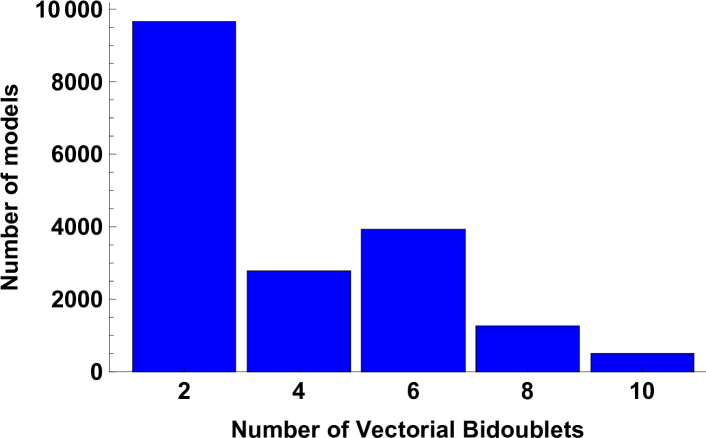
Figure 1: Number of three generation fertile cores versus number of twisted fertile vectorial representations from our set of 19374 fertile cores

The next step is the analysis of the LRS statistics resulting from our cores, which we obtain through a comprehensive scan of $\Pi_{2}$. The results are shown in Table 2. These results ought to be compared and contrasted to the results of the classification using the random classification method of [15], which are shown in a corresponding table on page 24 of ref. [15] for a sample of $10^{11}$ LRS vacua.

	Constraints	Total models in sample	Probability
	No Constraints	9919488	$1$
(1)	+ No Observable Enhancements	8894808	$0.9$
(2)	+ No Chiral Exotics	1699104	$0.17$
(3)	+ Complete Generations	1698818	$0.17$
(4)	+ Three Generations	827333	$8.3\times 10^{-2}$
(5)	+ SM Light Higgs	732728	$7.4\times 10^{-2}$
	& Heavy Higgs
(6)	+ Top Quark Mass Coupling	732728	$7.4\times 10^{-2}$
(7)	+ Minimal Heavy Higgs	141568	$1.4\times 10^{-2}$
	& Minimal SM Light Higgs

Table 2: Statistics for the LRS models derived from fertile cores

The methodology just described is analogous to that used in the Standard-Like Model classification of [14] except that here our comprehensive scan of $\Pi_{2}$ includes an analysis of the Enhanced, Hidden and Exotic sectors too. As mentioned in section 3.5, an important feature of our analysis was the inclusion of fertile cores which admitted an enhancement to the hidden sector gauge group. As can be seen in table 2 compared with Table 4 of [15], the probability of finding a model meeting all listed phenomenological criteria has increased from $4\times 10^{-11}$ to $1.4\times 10^{-2}$ due to our application of fertility conditions. This increase in probability by 9 orders of magnitude exhibits the power of the fertility methodology.

In order to explore the LRS statistics more closely, we can break down the results with respect to the important quantum numbers coming from the observable $\mathbf{16}$ representation and those coming from the vectorial $\mathbf{10}$ telling us the number of triplets and Higgs doublets at the LRS level. These statistics are presented in Table 3 for three generation models in which the number of triplets, $n_{3}$, and anti-triplets, $n_{\bar{3}}$, are matched.

5 Doublet-Triplet Splitting Discussion

One notable result from our analysis is that there are no examples of good models that are also triplet-free. After noting this result, we ran another scan of the $SO(10)$ space $\Pi_{1}$ in which we added a further fertility constraint on top of those listed in Section 3.4 such that there are no triplets or anti-triplets at the $SO(10)$ level, which can be expressed through the equation:

$$N_{10}^{t}=\frac{1}{2}\sum_{\begin{subarray}{c}A=1,2,3\\ p,q,r,s=0,1\end{subarray}}\left[1-C\left(V^{A}_{pqrs}\atop x\right)\right]R^{(A)}_{pqrs}=0.$$ (44)

In our analysis we found that the only fertile cores with no triplets were found contained net chirality $N_{L}-\overline{N}_{L}=N_{R}-\overline{N}_{R}=8$ and so can only give rise to four generation models. Therefore, triplet–free models with four generations are likely to exist and performing a fishing algorithm for such four generation, triplet–free models allowed us to find models such as the following:

$$(v_{i}|v_{j})=\blockarray{cccccccccccccc}&\mathds{1}Se_{1}e_{2}e_{3}e_{4}e_{5}e_{6}b_{1}b_{2}z_{1}z_{2}\alpha\\ \block{c(ccccccccccccc)}\mathds{1}111100111111-1/2\\ S1111111111111\\ e_{1}1100000001001\\ e_{2}1100000001101\\ e_{3}0100100100001\\ e_{4}0100010010001\\ e_{5}1100000000001\\ e_{6}1100100011001\\ b_{1}1000010111001\\ b_{2}1011000111001\\ z_{1}1101000000111\\ z_{2}1100000000111\\ \alpha 1111111100001\\$$ (45)

which is indeed triplet–free and four generation. This model also contains a top quark mass coupling, no chiral exotics, two heavy higgses, four standard model higgses and a hidden sector enhancement from the $z_{2}$ sector with oscillators $\{\bar{\phi}^{1234}\}$ enhancing the hidden group to $SU(6)\times SO(4)\times U(1)$.

$Q_{L}$	$Q_{R}$	$L_{L}$	$L_{R}$	$\bar{Q}_{L}$	$\bar{Q}_{R}$	$\bar{L}_{L}$	$\bar{L}_{R}$	$N_{h}$	$n_{3},n_{\bar{3}}$	Frequency
3	4	3	4	0	1	0	1	3	1	177152
3	4	3	4	0	1	0	1	3	3	167424
3	4	3	4	0	1	0	1	1	3	162304
3	4	3	4	0	1	0	1	1	5	91648
3	4	3	4	0	1	0	1	1	1	39424
3	4	3	4	0	1	0	1	5	1	38912
3	3	4	4	0	0	1	1	0	1	23488
4	4	3	3	1	1	0	0	0	1	23488
3	3	4	4	0	0	1	1	2	1	23488
3	4	4	3	0	1	1	0	0	1	23488
4	3	3	4	1	0	0	1	0	1	23488
3	4	4	3	0	1	1	0	2	1	23488
4	3	3	4	1	0	0	1	2	1	23488
4	4	3	3	1	1	0	0	2	1	23488
4	4	3	3	1	1	0	0	2	2	10624
4	3	3	4	1	0	0	1	2	2	10624
3	4	4	3	0	1	1	0	2	2	10624
3	3	4	4	0	0	1	1	2	2	10624
3	5	3	3	0	2	0	0	1	1	4864
3	3	3	5	0	0	0	2	1	1	4864
3	5	3	3	0	2	0	0	3	3	1792
3	3	3	5	0	0	0	2	3	3	1792
4	3	3	4	1	0	0	1	0	2	1328
3	3	4	4	0	0	1	1	4	2	1328
3	4	4	3	0	1	1	0	0	2	1328
4	4	3	3	1	1	0	0	4	2	1328

Table 3: LRS quantum number statistics for three generation models.

We note here that the doublet–triplet splitting mechanism, discussed in section 3.2, involves the projection of the sector $(2\alpha+x)$, on the observable vectorial states arising in the vectorial sectors in eq. (26). The $(2\alpha+x)$ projection breaks the underlying $SO(10)$ GUT symmetry to the Pati-Salam subgroup. Hence, a doublet–triplet splitting mechanism, similar to the one that we discussed here, is operational in the Pati–Salam, as well as the Standard–like, heterotic–string models, that employ a Pati–Salam symmetry breaking basis vector in the construction.

The absence of triplet-free three generation models in our sample may indicate that they are very rare, and hence are not generated in our statistical sampling, or may result from a deeper reason in the structure of the LRS heterotic–string models. Three generation triplet-free models may also exist in the PS and SLM heterotic–string models and can be searched for, by employing a similar analysis to that of section 3.2.

The fact that there are some four generation, triplet-free models though is somewhat reminiscent of the result for from the classification of FSU5 models in [12] that exophobic models exist only for even generation models.

It is also worth reiterating here that all the models obtained by using the free fermion classification method of refs [9, 10, 11, 12, 15] contain three pairs of vector–like triplet from the untwisted Neveu–Schwarz sector, due to the fact that all these models utilise symmetric boundary conditions for the set of worldsheet fermions $\{y,\omega|{\bar{y}},{\bar{\omega}}\}^{1,\cdots,6}$.

Projecting out the untwisted colour triplets and retaining the electroweak Higgs bidoublets, requires assignment of asymmetric boundary conditions for this set of worldsheet fermions, in the basis vector that breaks the $SO(10)$ symmetry to the Pati–Salam subgroup [23]. Implementation of the untwisted doublet-triplet splitting mechanism requires therefore extension of the classification method to free fermion models with asymmetric boundary conditions. Models which are free of both untwisted and twisted additional vector–like colour triplets may exist, but such models have not been generated to date.

Since the extra triplets appear in vector–like representation, mass terms can be generated from cubic level and higher order nonrenormalisable terms in the superpotential. In that case their masses may be intermediate, rather than at the Planck scale.

This situation is similar to that of the exotic fractionally charged states that are endemic in the heterotic–string models [29]. A phenomenological requirement on such states is that they appear in vector–like representations and are sufficiently massive or sufficiently rare to satisfy observational bounds. Models in which fractionally charged states appear only in the massive string spectrum, but not among the massless physical states, were dubbed as exophobic string models. Exophobic 3 generation models were found in the case of the PS heterotic–string models [11], but not in the cases of the FSU5 [12], the SLM [14], or the LRS [15], models. We may anticipate a similar situation with respect to the extra vector–like colour triplets that appear in these constructions.

6 Analysis of one Exemplary Model

It is interesting to examine in detail one of our 141568 exemplary models. As already mentioned, some of these models contain hidden enhancements but it’s preferable to select a minimal model with no enhancement. We also choose a model with a minimal number of exotics states. It would have been preferable to have found a model with none of the vectorial triplets/antitriplets but, as already mentioned, no good models were found to derive from fertile cores with no triplet/anti-triplets.

Using the notation convention:

$$C\binom{v_{i}}{v_{j}}=e^{i\pi(v_{i}|v_{j})}$$ (46)

the model defined by the following GGSO projection coefficients is an example of such a minimal model:

$$(v_{i}|v_{j})=\blockarray{cccccccccccccc}&\mathds{1}Se_{1}e_{2}e_{3}e_{4}e_{5}e_{6}b_{1}b_{2}z_{1}z_{2}\alpha\\ \block{c(ccccccccccccc)}\mathds{1}1100101110111.5\ \\ S1111111111111\ \\ e_{1}0111000101000\ \\ e_{2}0111000101010\ \\ e_{3}1100010000001\ \\ e_{4}0100110000000\ \\ e_{5}1100000000001\ \\ e_{6}1111000000110\ \\ b_{1}1000000010001\ \\ b_{2}0011000000001\ \\ z_{1}1100000100100\ \\ z_{2}1101000100010\ \\ \alpha 1100101000111\ \\$$ (47)

The observable matter sectors of this model produce three chiral generations, a top quark mass coupling, one SM Higgs and one heavy Higgs. There exists colour triplets from the vectorial 10 representation: one in the fundamental and one in the anti-fundamental, which pair up and obtain large mass. This model is free of chiral exotics and has 26 exotic states which is close to a minimum number of exotic states for LRS models since the classification done in [15] found 22 exotic states as a lower bound on exotics. In particular, in the notation of Table 1 from [15], there are no chiral exotics since the spinorial exotic numbers are $n_{L_{L^{s}}}=1=n_{\bar{L}_{L^{s}}}$ and $n_{L_{R^{s}}}=1=n_{\bar{R}_{L^{s}}}$, whilst the vectorial exotic numbers are $n_{3v}=1=n_{\bar{3}v}$ and $n_{1v}=5=n_{\bar{1}v}$. Additionally, the Pati-Salam exotic numbers are $n_{L_{L^{e}}}=4$ and $n_{L_{R^{e}}}=10$.

Another feature of this model is that it has an anomaly under the $U(1)_{2}$ and $U(1)_{3}$ gauge group factors since:

$$\operatorname{Tr}U(1)_{2}=12\ \ \ \text{and}\ \ \ \operatorname{Tr}U(1)_{3}=12$$ (48)

which results in an anomalous $U(1)$ combination of

$$U(1)_{A}=U(1)_{2}+U(1)_{3}.$$

We note here that the existence and profile of the anomalous $U(1)$ in this model is in contrast to the case of the LRS NAHE–based models that were constructed in ref. [7]. In the NAHE models, the $U(1)_{1,2,3}$ were found to be anomaly free. The reason is that the $\alpha$ projection selects opposite $U(1)_{j}$ charges for the left–handed and right–handed states from the sectors $b_{j}$. As a result, the sectors $b_{j}$ do not contribute to the anomaly. The same holds in the LRS models that we analyse here using our systematic classification method. The sectors $b_{j}$ therefore do not contribute to the anomalous $U(1)$ also in the models that are generated by eq. (2.2), and the contribution to the anomalous $U(1)$ arises from exotic states producing sectors.

7 Conclusion

The left–right symmetric models represent an appealing extension of the Standard Model [30] restoring the left–right symmetry in its spectrum, and attributing its violation to spontaneous symmetry breaking. Furthermore, it mandates the existence of right–handed neutrinos and has a natural embedding in $SO(10)$. From the point of view of heterotic–string model building they also represent an interesting case, as they do not follow from the more common $SO(12)\times E_{8}\times E_{8}$ route, but rather from the pattern $SO(16)\times E_{7}\times E_{7}$ [7]. Resulting in models in which all $U(1)$ symmetries are anomaly free [7], and in particular ${\rm Tr}U(1)_{1,2,3}=0$. In this paper, we presented a model with ${\rm Tr}U(1)_{1}={\rm Tr}U(1)_{2}\neq 0$, in which case the contribution to the anomalies arises from exotic states producing sectors.

In terms of the fermionic $Z_{2}\times Z_{2}$ classification program the LRS models present challenges that are similar to the SLM classification. In both cases there is a proliferation of exotic states producing sectors, lowering the frequency of viable three generation models in the total space of models. For that purpose, one identifies fertile conditions at the $SO(10)$ level and selects cores that are amenable to producing three generation configurations. Around these fertile cores a complete classification of the $SO(10)$ breaking phases is performed. In ref. [15] a classification using the random generation method was performed producing a small number of three generation models. Adopting the two stage classification method in this paper, the number of viable models is increased by four orders of magnitude. Furthermore, we showed that the fertility conditions are associated with a novel doublet–triplet splitting mechanism that operates in the twisted sectors of the LRS vacua. While a doublet–triplet splitting was demonstrated in the past for untwisted states [23], the doublet–triplet splitting mechanism identified herein operates in the twisted sectors, and may be employed in SLM and PS heterotic–string models as well. The stage is now ripe for adopting novel computational methods in the classification program [31] to identify patterns in the GGSO coefficient space that are conducive for producing viable phenomenological characteristics.

References

- [1] For review and references see e.g: L.E Ibanez and A.M Uranga, String theory and particle physics: an introduction to string phenomenology, Cambridge University Press, 2012.
-
[2]
P. Candelas, G.T. Horowitz, A. Strominger and E. Witten,
Nucl. Phys. B258 (1985) 46;
D.J. Gross, J.A. Harvey, E.J. Martinec and R. Rohm, Nucl. Phys. B267 (1986) 75. -
[3]
A.E. Faraggi, Phys. Lett. B326 (1994) 62; Phys. Lett. B544 (2002) 207;
E. Kiritsis and C. Kounnas, Nucl. Phys. B503 (1997) 117;
A.E. Faraggi, S. Forste and C. Timirgaziu, JHEP 0608 (2006) 057;
P. Athanasopoulos, A.E. Faraggi, S. Groot Nibbelink and V.M. Mehta, JHEP 1604 (2016) 038. - [4] I. Antoniadis, J. Ellis, J. Hagelin and D.V. Nanopoulos, Phys. Lett. B231 (1989) 65
-
[5]
A.E. Faraggi, D.V. Nanopoulos and K. Yuan,
Nucl. Phys. B335 (1990) 347;
A.E. Faraggi, Phys. Lett. B278 (1992) 131; Nucl. Phys. B387 (1992) 239;
G.B. Cleaver, A.E. Faraggi and D.V. Nanopoulos, Phys. Lett. B455 (1999) 135;
A.E. Faraggi, E. Manno and C.M. Timirgaziu, Eur. Phys. Jour. C50 (2007) 701. -
[6]
I. Antoniadis. G.K. Leontaris and J. Rizos,
Phys. Lett. B245 (1990) 161;
G.K. Leontaris and J. Rizos, Nucl. Phys. B554 (1999) 3. -
[7]
G.B. Cleaver, A.E. Faraggi and C. Savage, Phys. Rev. D63 (2001) 066001;
G.B. Cleaver, D.J Clements and A.E. Faraggi, Phys. Rev. D65 (2002) 106003; - [8] A. Gregori, C. Kounnas and J. Rizos, Nucl. Phys. B549 (1999) 16.
- [9] A.E. Faraggi, C. Kounnas, S.E.M Nooij and J. Rizos, hep-th/0311058; Nucl. Phys. B695 (2004) 41.
- [10] A.E. Faraggi, C. Kounnas and J. Rizos, Phys. Lett. B648 (2007) 84; Nucl. Phys. B774 (2007) 208; Nucl. Phys. B799 (2008) 19.
-
[11]
B. Assel, C. Christodoulides, A.E. Faraggi, C. Kounnas and J. Rizos
Phys. Lett. B683 (2010) 306; Nucl. Phys. B844 (2011) 365;
C. Christodoulides, A.E. Faraggi and J. Rizos, Phys. Lett. B702 (2011) 81. - [12] A.E. Faraggi, J. Rizos and H. Sonmez, Nucl. Phys. B886 (2014) 202.
- [13] H. Sonmez, Phys. Rev. D93 (2016) 125002.
- [14] A.E. Faraggi, J. Rizos and H. Sonmez, Nucl. Phys. B927 (2018) 1.
- [15] A.E. Faraggi, G. Harries and J. Rizos, Nucl. Phys. B936 (2018) 472, arXiv:1806.04434.
-
[16]
T. Catelin-Julian, A.E. Faraggi, C. Kounnas and J. Rizos,
Nucl. Phys. B812 (2009) 103;
C. Angelantonj, A.E. Faraggi and M. Tsulaia, JHEP 1007 (2010) 314;
A.E. Faraggi, I. Florakis, T. Mohaupt and M. Tsulaia, Nucl. Phys. B848 (2011) 332. - [17] P. Athanasoupoulos, A.E. Faraggi and D. Gepner, Phys. Lett. B735 (2014) 357.
- [18] L. Bernard et al, Nucl. Phys. B868 (2013) 1.
-
[19]
A.E. Faraggi and J. Rizos, Nucl. Phys. B895 (2015) 233;
A.E. Faraggi and J. Rizos, Eur. Phys. Jour. C76 (2016) 170;
J. Ashfaque, L. Delle Rose, A.E. Faraggi and C. Marzo, Eur. Phys. Jour. C76 (2016) 570. -
[20]
See e.g.: D. Senechal, Phys. Rev. D39 (1989) 3717;
K.R. Dienes, Phys. Rev. Lett. 65 (1990) 1979; Phys. Rev. D73 (2006) 106010;
M.R. Douglas, JHEP 0305 (2003) 046;
R. Blumenhagen et al, Nucl. Phys. B713 (2005) 83;
F. Denef and M.R. Douglas, JHEP 0405 (2004) 072;
T.P.T. Dijkstra, L. Huiszoon and A.N. Schellekens, Nucl. Phys. B710 (2005) 3;
B.S. Acharya, F. Denef and R. Valadro, JHEP 0506 (2005) 056;
P. Anastasopoulos, T.P.T. Dijkstra, E. Kiritsis and A.N. Schellekens, Nucl. Phys. B759 (2006) 83;
M.R. Douglas and W. Taylor, JHEP 0701 (2007) 031;
K.R. Dienes, M. Lennek, D. Senechal and V. Wasnik, Phys. Rev. D75 (2007) 126005;
O. Lebedev et al, Phys. Lett. B645 (2007) 88;
E. Kiritsis, M. Lennek and A.N. Schellekens JHEP 0902 (2009) 030;
L.B. Anderson, A. Constantin, J. Gray, A. Lukas and E. Palti, JHEP 1401 (2014) 047;
J. Halverson and P. Langacker, PoS TASI2017 (2018) 019, arXiv:1801.03053. - [21] S. Abel and J. Rizos, JHEP 1408 (2014) 10.
-
[22]
O. Lebedev et al, Phys. Rev. D77 (2008) 046013;
A. Mẗter, E. Parr and P.K.S. Vaudrevange, Nucl. Phys. B940 (2019) 113y;
E. Parr and P.K.S. Vaudrevange, arxiv:1910.13473; - [23] A.E. Faraggi, Nucl. Phys. B428 (1994) 111; Phys. Lett. B520 (2001) 337;
-
[24]
I. Antoniadis, C. Bachas, and C. Kounnas, Nucl. Phys. B289 (1987) 87;
H. Kawai, D.C. Lewellen, and S.H.-H. Tye, Nucl. Phys. B288 (1987) 1;
I. Antoniadis and C. Bachas, Nucl. Phys. B298 (1988) 586. - [25] A.E. Faraggi and H. Sonmez, Phys. Rev. D91 (066006) 2015
- [26] K. Abe, et al., Phys. Rev. D95 (2017) 012004
- [27] A.E. Faraggi and D.V. Nanopoulos, Phys. Rev. D48 (1993) 3288.
- [28] J. Rizos, Eur. Phys. Jour. C74 (2014) 2905
-
[29]
X.G. Wen and E. Witten, Nucl. Phys. B261 (1985) 651;
A. Schellekens, Phys. Lett. B237 (1990) 363;
A.E. Faraggi, Phys. Rev. D46 (1992) 3204;
S. Chang, C. Coriano and A.E. Faraggi, Nucl. Phys. B477 (1996) 65. -
[30]
A. Salam and J.C. Pati, Phys. Rev. D10 (1975) 275:
R.N. Mohapatra and J.C. Pati, Phys. Rev. D11 (1975) 566; Phys. Rev. D11 (1975) 2558. - [31] A.E. Faraggi, G. Harries, B. Percival and J. Rizos, arXiv:1901.04448.