Generalised Network Autoregressive Processes and the GNAR package

Marina Knight, Kathryn Leeming, Guy Nason, Matthew Nunes Generalised Network Autoregressive Processes and the GNAR package GNAR processes This article introduces the GNAR package, which fits, predicts, and simulates from a powerful new class of generalised network autoregressive processes. Such processes consist of a multivariate time series along with a real, or inferred, network that provides information about inter-variable relationships. The GNAR model relates values of a time series for a given variable and time to earlier values of the same variable and of neighbouring variables, with inclusion controlled by the network structure. The GNAR package is designed to fit this new model, while working with standard ts objects and the igraph package for ease of use. multivariate time series, networks, missing data, network time series multivariate time series, networks, missing data, network time series Marina Knight
Department of Mathematics
University of York, UK
E-mail:
URL: https://www.york.ac.uk/maths/staff/marina-knight/ and
Kathryn Leeming
Department of Statistics
University of Warwick, UK
E-mail:
URL: https://www.warwick.ac.uk/fac/sci/statistics/staff/academic-research/leeming/ and
Guy P. Nason
Department of Mathematics
Imperial College London, UK
E-mail:
URL: http://www.imperial.ac.uk/people/g.nason and
Matthew Nunes
School of Mathematical Sciences
University of Bath, UK. E-mail:
URL: http://people.bath.ac.uk/man54/

1 Introduction

Increasingly within the sciences, networks and network methodologies are being used to answer research questions. Such networks might be observed, such as connections in communication network or information flows within, or they could be unobserved: inferred networks that can explain a process or effect. Given the increase in the size of data sets, it may also be useful to infer a network from data to efficiently summarise the data generating process.

We consider time series observations recorded at different nodes of a network, or graph. Our GNAR package (leeming18:GNAR) and its novel generalised network autoregressive (GNAR) statistical models focus on partnering a network with a multivariate time series and modelling them jointly. One can find an association network, see, e.g., Chapter 7 of Kolaczyk2009, or Granger causality network, e.g., Dahlhaus2003, between different variables by analysing a multivariate time series and its properties. However, here we assume the existence of an underlying network and use it during the analysis of the time series, although sometimes its complete structure is unknown.

Networks can provide strong information about the dependencies between variables. Within our generalised network autoregressive (GNAR) model, each node depends on its previous values as in the univariate autoregressive framework, but also may depend on the previous values at its neighbours, neighbours of neighbours, and so on. Our GNAR modelling framework is flexible, allowing for different types of network, networks that change their structure over time (time-varying networks), and also can be powerfully applied in the important practical situation where the time series feature missing observations.

Driven in part by the increased popularity and recent research activity in the field of statistical network analysis, there has been a concurrent growth in software for analysing such data. An exhaustive list of these packages is beyond the scope of this article, but we review some relevant ones here.

Existing software in this area predominantly focusses on the various models for network-structured data. In the static network setting, these include packages dedicated to latent space network models, such as collpcm (wyse17:collpcm), HLSM (adhikari18:HLSM), latentnet (krvitsky18:latentnet) amongst others; exponential random graph models and their variants, for example ergm (handcock18:ergm), GERGM (denny18:GERGM) or hergm (schweinberger18:hergm); and block models in e.g., blockmodels (leger15:blockmodels). For dynamic networks, packages for time-varying equivalents of these network models are also available, see e.g., the tergm package (krvitsky18:tergm) or dynsbm (matias18:dynsbm). There are also a multitude of more general packages for network analysis, e.g., for network summary computation or implementations of methodology in specific applications of interest.

Despite this, software dedicated to the analysis of time series and other processes on networks is sparse. A number of packages implement epidemic (e.g., SIR) models of disease spread, notably epinet (groendyke18:epinet), EpiLM/EpiLMCT (warriyar18:EpiLM; almutiry18:EpiLMCT) and hybridModels (marquez18:hybridModels); these use transmission rates to model processes as opposed to temporal and network dependence through time series models as in GNAR. Similarly, the NetOrigin software (manitz18:NetOrigin) is dedicated to source estimation for propagation processes on networks, rather than fitting time series models. Packages such as networkTomography (blocker14:networkTomography) deal with time-varying models for (discrete) count processes or flows on links of a fixed routing network; the tnam package (leifeld17:tnam) fits models using spatial (and not network-node) dependence. Both of these are in contrast to the GNAR package, which implements time series models which account for known time-varying network structures.

Other packages can implicitly develop network-like structured time series models through penalised or constrained variable selection, such as autovarCore (emerencia18:autovarCore), nets (brownlees17:nets), sparsevar (vazoller16:sparsevar), as well as the vars package (Pfaff2008). Packages that take a graphical modelling approach to the dependence structure within time series include gimme (lane19:gimme), graphicalVAR (epskamp18:graphicalVAR), mgm (haslbeck19:mgm), mlVAR (epskamp19:mlVAR), and sparseTSCGM (abegaz16:sparseTSCGM). These approaches also differ fundamentally from the GNAR models since the network is constructed during analysis, as opposed to GNAR, which specifically incorporates information on the network structure into the model a priori. The vars package features in Section 4.2, where we highlight the differences between the GNAR models and this existing class of techniques.

Section 2 introduces our model, and demonstrates how GNAR can be used to fit network models to simulated network time series in Section 2.4. Order selection and prediction are discussed in Section 3, which includes an example of how to use BIC to select model order for a wind speed network time series in Section 3.2. An extended example, concerning constructing a network to aid GDP forecasting, is presented in Section 4. Section LABEL:Discussion discusses different network modelling options that could be chosen, and presents a summary of the article. All results were calculated using version 3.5.1 of the statistical software R (Rcore2017).

2 Network time series processes

We assume that our multivariate time series follows an autoregressive-like model at each node, depending both on the previous values of the process at that node, and on neighbouring nodes at previous time steps. These neighbouring nodes are included as part of the network structure, as defined below.

2.1 Network terminology and notation

Throughout we assume the presence of one or more networks, or graphs, associated with the observed time series. Each univariate time series that makes up the multivariate time series occurs, or is observed at, a node, or location on the graph(s). These nodes are connected by a set of edges, which may be directed, and/or weighted.

We denote a graph by $\mathcal{G}=(\mathcal{K},\mathcal{E})$, where $\mathcal{K}=\{1,...,N\}$ is the set of nodes, and $\mathcal{E}$ is the set of edges. A directed edge from node $i\in\mathcal{K}$ to $j\in\mathcal{K}$ is denoted $i\rightsquigarrow j$, and an un-directed edge between the nodes is denoted $i\leftrightsquigarrow j$. The edge set of a directed graph is $\mathcal{E}=\{(i,j):i\rightsquigarrow j;i,j\in\mathcal{K}\}$, and similarly for the set of un-directed edges.

2.1.1 Stage-$r$ neighbourhoods

We introduce the notion of neighbours and stage-neighbours in the graph structure as follows; for a subset $A\subset\mathcal{K}$ the neighbour set of $A$ is given by $\mathcal{N}(A)=\{j\in\mathcal{K}/A:i\rightsquigarrow j;i\in A\}$. These are the first neighbours, or stage-1 neighbours of $A$. The $r$th stage neighbours of a node $i\in\mathcal{K}$ are given by $\mathcal{N}^{(r)}(i)=\mathcal{N}\{\mathcal{N}^{(r-1)}(i)\}/[\{\cup_{q=1}^{r-1}\mathcal{N}^{(q)}(i)\}\cup\{i\}]$, for $r=2,3,...$ and $\mathcal{N}^{(1)}(i)=\mathcal{N}(\{i\})$.

Figure 1 shows an example graph, where node E has stage-1 neighbour A, stage-2 neighbour D, and stage-3 neighbours B and C. Neighbour sets for this example include $\mathcal{N}^{(1)}(D)=\{A,B,C\}$, and $\mathcal{N}^{(3)}(E)=\{B,C\}$. In the time-varying network setting, a subscript $t$ is added to the neighbour set notation.

2.1.2 Connection weights

Each network can have connection weights $\omega\in[0,1]$ associated with every pair of nodes. This connection weight can depend on the size of the neighbour set and also encodes any edge-weight information. Formally, the values of the connection weights from a node $i\in\mathcal{K}$ to its stage-$r$ neighbour $j\in\mathcal{N}^{(r)}(i)$ will be the reciprocal of the number of stage-$r$ neighbours; $\omega_{i,j}=|\mathcal{N}^{(r)}(i)|^{-1}$, where $|\cdot|$ denotes the cardinality of a set. In Figure 1 the connection weights would be, for example, $\omega_{E,A}=1$, $\omega_{A,E}=\omega_{A,D}=0.5$. Connection weights are not necessarily symmetric, even for an un-directed graph. We note that this choice of these inverse distance weights is one of many possibilities, and some other means of creating connection weights could be used.

When the edges are weighted, or have a distance associated with them, we use the concept of distance to find the shortest path between two vertices. Let the distance from node $i$ to $\ell$ be denoted $d_{i,\ell}\in\mathbb{R}_{+}$, and if there is an un-normalised weight between these nodes, denote this $\mu_{i,\ell}\in\mathbb{R}_{+}$. To find the length of connection between a node $i$ and its stage-$r$ neighbour, $k$, we sum the distances on the paths with $r$ edges from $i$ to $k$ and take the minimum (note that there are no paths with fewer edges than $r$ as $k$ is a stage-$r$ neighbour). If the network includes weights rather than distances, we find the shortest $r$ length path where $d_{i,\ell}=\mu_{i,\ell}^{-1}$. Then the connection weights between node $i$ and its stage-$r$ neighbour $k$ are either $\omega_{i,k}=d_{i,k}^{-1}\{\sum_{\ell\in\mathcal{N}^{(r)}(i)}d_{i,\ell}^{-1}\}^{-1}$ for distances, or $\omega_{i,k}=\mu_{i,k}\{\sum_{\ell\in\mathcal{N}^{(r)}(i)}\mu_{i,\ell}\}^{-1}$ for a network with weights. This definition means that all nodes will have connection weights that sum to one for any non-empty neighbour set, whether they are in a sparse or dense part of the graph.

2.1.3 Edge or node covariates

A further important innovation permits a covariate that can be used to encode edges effects (or nodes) into certain types. Our covariate will take $C\in\mathbb{N}$ discrete values and be indexed by $c$. A more general covariate could be considered, but we wish to keep our notation simple in the definition that follows. For example, in an epidemiological network we might have two edge types: one that carries information about windborne spread of infection and the other carries information about identified direct infections. The covariates do not change our neighbour sets or connection weight definitions, so we have the property $\sum\limits_{q\in\mathcal{N}^{(r)}(i)}\sum\limits_{c=1}^{C}\omega_{i,q,c}=1$ for all $i\in\mathcal{K}$ and $r\in\mathbb{N}$ such that $\mathcal{N}^{(r)}(i)$ is non-empty.

2.2 The generalised network autoregressive model

Consider an $N\times 1$ vector of nodal time series, $\mathbf{X}_{t}=(X_{1,t},\ldots,X_{N,t})^{\prime}$, where $N$ is considered fixed. Our aim is to model the dependence structure within and between the nodal series using the network structure provided by (potentially time-varying) connection weights, $\omega$. For each node $i\in\{1,\ldots,N\}$ and time $t\in\{1,\ldots,T\}$, our generalised autoregressive model of order $(p,[\mathbf{s}])\in\mathbb{N}\times\mathbb{N}_{0}^{p}$ for $\mathbf{X}_{t}$ is

$$X_{i,t}=\sum_{j=1}^{p}\left(\alpha_{i,j}X_{i,t-j}+\sum_{c=1}^{C}\sum_{r=1}^{s_{j}}\beta_{j,r,c}\sum_{q\in\mathcal{N}^{(r)}_{t}(i)}\omega_{i,q,c}^{(t)}X_{q,t-j}\right)+u_{i,t},$$ (1)

where $p\in\mathbb{N}$ is the maximum time lag, $[\mathbf{s}]=(s_{1},\ldots,s_{p})$ and $s_{j}\in\mathbb{N}_{0}$ is the maximum stage of neighbour dependence for time lag $j$, with $\mathbb{N}_{0}=\mathbb{N}\cup\{0\}$, $\mathcal{N}^{(r)}_{t}(i)$ is the $r$th stage neighbour set of node $i$ at time $t$, $\omega_{i,q,c}^{(t)}\in[0,1]$ is the connection weight between node $i$ and node $q$ at time $t$ if the path corresponds to covariate $c$. Here, we consider a sum from one to zero to be zero, i.e., $\sum_{r=1}^{0}(\cdot)\coloneqq 0$. The $\alpha_{i,j}\in\mathbb{R}$ are ‘standard’ autoregressive parameters at lag $j$ for node $i$. The $\beta_{j,r,c}\in\mathbb{R}$ correspond to the effect of the $r$th stage neighbours, at lag $j$, according to covariate $c=1,\ldots,C$. Later, we derive conditions on the model parameters to achieve process stationarity over the network. Here the noise, $\{u_{i,t}\}$, is assumed to be independent and identically distributed at each node $i$, with mean zero and variance $\sigma_{i}^{2}$. Our model meaningfully enhances that of the arXiv publication Knight2016 by now additionally including different autoregressive parameters, connection weights at each node and, particularly, parameters $\beta$ that depend on covariates. Note that the IID assumption on the noise $\{u_{i,t}\}$ could of course be relaxed to include correlated innovations.

We note that crucially, the time-dependent network topology is integral to the model parametrisation through the use of time-varying weights and neighbours. These features yield a model that is sensitive to the network structures and captures contemporaneous as well as autoregressive relationships, as defined by equation (1). The network should therefore be viewed not as an estimable quantity, but as a time-dependent known structure.

In the GNAR model, the network may change over time, but the covariates stay fixed. This means that the underlying network can be altered over time, for example, to allow for nodes to drop in and out of the series but model fitting can still be carried out. Practically, this is extremely useful, as shown by the example in Section 4. Our model allows for the $\alpha$ parameters may be different at each node, however the interpretation of the network regression parameters, $\beta_{j,r,c}$, is the same throughout the network.

A more restrictive version of the above model is the global-$\alpha$ GNAR$(p,[\textbf{s}])$ model, which has the same autoregressive covariate at each node, where the $\alpha_{i,j}$ are replaced by $\alpha_{j}$. This defines a process with the same behaviour at every node, with differences being present only due to the graph structure.

2.3 GNAR network example

Networks in the GNAR package are stored in a list with two components edges and dist. The edges component is itself a list with $N$ slots each containing a vector whose entries are indices to their neighbouring nodes. For example, if $3\leftrightsquigarrow 4$ denotes an undirected edge between nodes $3$ and $4$ then the vector edges[[3]] will contain a 4 and edges[[4]] will contain a 3. If the network is undirected this will mean that each edge is ‘double counted’ in summary information. A directed edge $3\rightsquigarrow 4$ would be listed in edges[[3]] as a 4, but not edges[[4]] if there is no edge in the opposite direction. The dist component is of the same format as edges, and contains the distances corresponding to the edge links, if they exist. For example, in an un-weighted setting, the connection weights are such that all neighbours of a node have equal effect on the node. This is achieved by setting all entries of the dist component to one, and the software calculates the connection weight from these. A GNAR network is stored in a GNARnet object, and an object can be checked using the is.GNARnet function. The S3 methods plot, print, and summary are available for GNARnet objects.

Figure 1 shows an example that is stored as a GNARnet object called fiveNet and can be reproduced using R> library("GNAR") R> library("igraph") R> plot(fiveNet, vertex.label = c("A", "B", "C", "D", "E"))

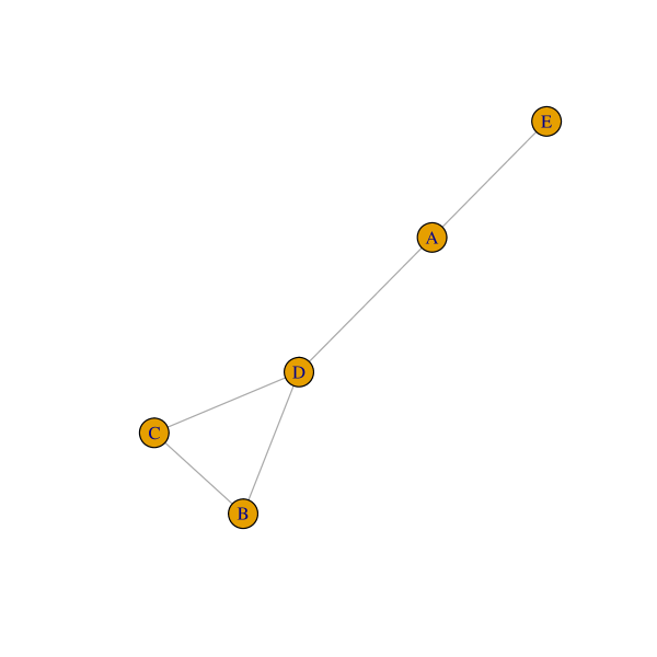
Figure 1: An example un-directed, un-weighted graph with five nodes labelled A to E.

The basic structure of the GNARnet object is, as usual, displayed with R> summary(fiveNet) GNARnet with 5 nodes and 10 edges of equal length 1

2.3.1 Converting a network to GNARnet form

Our GNARnet format integrates with other methods of specifying a network via a set of functions that generate a GNARnet from others, such as an igraph object.

An igraph object can be converted to and from the GNARnet structure using the functions igraphtoGNAR and GNARtoigraph, respectively. For example, starting with the fiveNet GNARnet object, R> fiveNet2 <- GNARtoigraph(net = fiveNet) R> summary(fiveNet2) IGRAPH 41ddef8 U-W- 5 5 – + attr: weight (e/n) R> fiveNet3 <- igraphtoGNAR(fiveNet2) R> all.equal(fiveNet, fiveNet3) [1] TRUE whereas the reverse conversion would be performed as R> g <- make_ring(10) R> print(igraphtoGNAR(g)) GNARnet with 10 nodes edges:1–2 1–10 2–1 2–3 3–2 3–4 4–3 4–5 5–4 5–6 6–5 6–7 7–6 7–8 8–7 8–9 9–8 9–10 10–1 10–9

edges of each of length 1 We can also use the GNARtoigraph function to extract graphs involving higher-order neighbour structures, for example, creating a network of third-order neighbours.

In addition to interfacing with igraph, we can convert between GNARnet objects and adjacency matrices using functions as.matrix and matrixtoGNAR. We can produce an adjacency matrix for the fiveNet object with R> as.matrix(fiveNet) [,1] [,2] [,3] [,4] [,5] [1,] 0 0 0 1 1 [2,] 0 0 1 1 0 [3,] 0 1 0 1 0 [4,] 1 1 1 0 0 [5,] 1 0 0 0 0 and an example converting a weighted adjacency matrix to a GNARnet object is R> adj <- matrix(runif(9), ncol = 3, nrow = 3) R> adj[adj < 0.3] <- 0 R> print(matrixtoGNAR(adj)) GNARnet with 3 nodes edges:1–1 1–3 2–2 3–1 3–2 edges of unequal lengths

2.4 Example: GNAR model fitting

The fiveNet network has a simulated multivariate time series associated with it of class ts called fiveVTS. The pair together are a network time series. The object can be loaded in the usual way using the data function. GNAR contains functions for fitting and predicting from GNAR models: GNARfit and the predict method, respectively. These make use of the familiar R command lm, since the GNAR model can be essentially re-formulated as a linear model, as we shall see in Section 3 and Appendix LABEL:consistency. As such, least squares variance / standard error computations are also readily obtained, although other, e.g., HAC-type variance estimators could also be considered for GNAR models.

Suppose we wish to fit the global-$\alpha$ network time series model GNAR$(2,[1,1])$, a model with four parameters in total. We can fit this model with the following code. R> data("fiveNode") R> answer <- GNARfit(vts = fiveVTS, net = fiveNet, alphaOrder = 2, + betaOrder = c(1, 1)) R> answer Model: GNAR(2,[1,1])

Call: lm(formula = yvec   dmat + 0)

Coefficients: dmatalpha1 dmatbeta1.1 dmatalpha2 dmatbeta2.1 0.20624 0.50277 0.02124 -0.09523 In this fit, the global autoregressive parameters are $\hat{\alpha}_{1}\approx 0.206$ and $\hat{\alpha}_{2}\approx 0.021$ and the $\beta$ network parameters are $\hat{\beta}_{1,1,1}\approx 0.503$ and $\hat{\beta}_{2,1,1}\approx-0.095$. Also, the network edges only have one type of covariate so $C=c=1$. We can just look at one node. For example, the model at node A is

$$X_{A,t}=0.206X_{A,t-1}+0.503(X_{E,t-1}+X_{D,t-1})/2+0.021X_{A,t-2}-0.095(X_{E,t-2}+X_{D,t-2})/2+u_{E,t}.$$

The model coefficients can be extracted from a GNARfit object using the coef function as is customary. The GNARfit object returned by GNARfit function also has methods to extract fitted values and the residuals. For example, Figure 2 shows the first node time series and the residuals from fitting the model. Figure 2 was produced by R> plot(fiveVTS[, 1], ylab = "Node A Time Series") R> lines(fitted(answer)[, 1], col = 2)

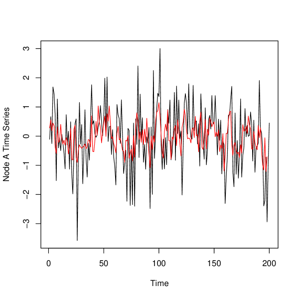
Figure 2: Time series of first node (black) with fitted values from ‘answer’ model overlaid in red.

Alternatively, we can examine the associated residuals: R> myresiduals <- residuals(answer)[, 1] R> layout(matrix(c(1, 2), 2, 1)) R> plot(ts(residuals(answer)[, 1]), ylab = "‘answer’ model residuals") R> hist(residuals(answer)[, 1], main = "", + xlab = "‘answer’ model residuals")

Figure 3: Residual plots from ‘answer’ model fit. Top: Time series; Bottom: Histogram.

By altering the input parameters in the GNARfit function, we can fit a range of different GNAR models and the reader can consult Appendix LABEL:extrasims for further examples.

2.5 Example: GNAR data simulation on a given network

The following example demonstrates network time series simulation using the network in Figure 1.

Model (a) is a GNAR$(1,[1])$ model with individual $\alpha$ parameters, $(\alpha_{A,1},\alpha_{B,1},\alpha_{C,1},\alpha_{D,1},\alpha_{E,1})=(0.4,0,-0.6,0,0)$, and the same $\beta$ parameter throughout, $\beta_{1}=0.3$. Model (b) is a global-$\alpha$ GNAR$(2,[2,0])$ model with parameters $\alpha_{1}=0.2$, $\beta_{1,1}=0.2$, $\beta_{1,2}=0.3$ and $\alpha_{2}=0.3$. Both simulations are created using standard normal noise whose standard deviation is controlled using the sigma argument. R> set.seed(10) R> fiveVTS2 <- GNARsim(n = 200, net = fiveNet, + alphaParams = list(c(0.4, 0, -0.6, 0, 0)), betaParams = list(c(0.3))) By fitting an individual-alpha GNAR$(1,[1])$ model to the simulated data with the fiveNet network, we can see that these estimated parameters are similar to the specified ones of 0.4, 0, -0.6, 0, 0 and 0.3. This agreement does not come as a surprise given that we show theoretical consistency for parameter estimators (see Appendix LABEL:consistency).

R> print(GNARfit(vts = fiveVTS2, net = fiveNet, alphaOrder = 1, + betaOrder = 1, globalalpha = FALSE)) Model: GNAR(1,[1])

Call: lm(formula = yvec   dmat + 0)

Coefficients: dmatalpha1node1 dmatalpha1node2 dmatalpha1node3 dmatalpha1node4 0.45902 0.13133 -0.49166 0.03828 dmatalpha1node5 dmatbeta1.1 0.02249 0.24848

Repeating the experiment for the GNAR(2, [2, 0]) Model (b), the estimated parameters are again similar to the generating parameters:

R> set.seed(10) R> fiveVTS3 <- GNARsim(n = 200, net = fiveNet, + alphaParams = list(rep(0.2, 5), rep(0.3, 5)), + betaParams = list(c(0.2, 0.3), c(0))) R> print(GNARfit(vts = fiveVTS3, net = fiveNet, alphaOrder = 2, + betaOrder = c(2,0))) Model: GNAR(2,[2,0])

Call: lm(formula = yvec   dmat + 0)

Coefficients: dmatalpha1 dmatbeta1.1 dmatbeta1.2 dmatalpha2 0.2537 0.1049 0.3146 0.2907

Alternatively, we can use the simulate S3 method for GNARfit objects to simulate time series associated to a GNAR model, for example R> fiveVTS4 <- simulate(GNARfit(vts = fiveVTS2, net = fiveNet, + alphaOrder = 1, betaOrder = 1, globalalpha = FALSE), n = 200)

2.6 Missing data and changing connection weights with GNAR models

Standard multivariate time series models, including vector autoregressions (VAR), can have significant problems in coping with certain types of missingness and imputation is often used, see Guerrero10, Honaker10, Bashir16. While in VAR modelling successful solutions have been found to cope with specific missingness scenarios, such as implemented in the gimme R package (lane19:gimme), however, if a variable has e.g., block missing data, the coefficients corresponding that variable can be difficult to calculate, and impossible if their partner variable is missing at cognate times. In addition, due to computational burden gimme is limited to modelling a single time lag. A key advantage of our parsimonious GNAR model is that it models via neighbourhoods across the entire data set. If a node is missing for a given time, then it does not contribute to the estimation of neighbourhood parameters that the network structure suggests it should, and there are plenty of other nodes that do contribute, generally resulting in a high number of observations to estimate each coefficient. In GNAR models, missing data of this kind is not a problem.

The flexibility of GNAR modelling means that we can also model missing data as a changing network, or alternatively, as changing connection weights. In the situation where the overall network is considered fixed, but when observations are missing at particular nodes, the connections and weightings need altering accordingly. Again, using the graph in Figure 1, consider the situation where node A does not have any data recorded. Yet, we want to preserve the stage-2 connection between D and E, and the stage-3 connection between E and both B and C. To do this, we do not redraw the graph and remove node A and its connections, instead we reweight the connections that depend on node A. As node A does not feature in the stage-2 or stage-3 neighbours of E, the connection weights $\omega_{E,D},\omega_{E,B},\omega_{E,C}$ do not change, but the connection weight $\omega_{E,A}$ drops to zero in the absence of observation from node A. Similarly, the stage-1 neighbours of D are changed without A, so $\omega_{D,A}$ drops to zero and the other two connection weights from node D increase accordingly; $\omega_{D,B}=\omega_{D,C}=0.5$.

Missing data of this kind is handled automatically by the GNAR functions using customary NA missing data values present in the vts (vector time series) component of the overall network time series. For example, inducing some (artificial) missingness in the fiveVTS series, we can still obtain estimates of model parameters: R> fiveVTS0 <- fiveVTS R> fiveVTS0[50:150, 3] <- NA R> nafit <- GNARfit(vts = fiveVTS0, net = fiveNet, alphaOrder = 2, + betaOrder = c(1, 1)) R> layout(matrix(c(1, 2), 2, 1)) R> plot(ts(fitted(nafit)[, 3]), ylab = "Node C fitted values") R> plot(ts(fitted(nafit)[, 4]), ylab = "Node D fitted values")

Figure 4: Fitted values of global-$\alpha$ GNAR$(1,[1])$ fit to the ‘fiveVTS’ data, with observations 50–150 removed from node C. Fitted values: Top: Node C; Bottom: Node D.

As shown in Figure 4, after removing observations from the time series at node C, its neighbour, node D, still has a complete set of fitted values.

2.7 Stationarity conditions for a GNAR process with fixed network

Theorem 1

Given an unchanging network, $\mathcal{G}$, a sufficient condition for the GNAR model (1) to be stationary is

$$\sum_{j=1}^{p}\left(|\alpha_{i,j}|+\sum\limits_{c=1}^{C}\sum\limits_{r=1}^{s_{j}}|\beta_{j,r,c}|\right)<1\quad\forall i\in 1,...,N.$$ (2)

The proof of Theorem 1 can be found in Appendix LABEL:appstatcon.

For the global-$\alpha$ model this condition reduces to

$${\sum_{j=1}^{p}\left(|\alpha_{j}|+\sum\limits_{c=1}^{C}\sum\limits_{r=1}^{s_{j}}|\beta_{j,r,c}|\right)<1}.$$ (3)

We can explore these conditions using the GNARsim function. The following example uses parameters whose absolute value sums to greater than one and then we calculate the mean over successive time periods. The mean increases rapidly indicating nonstationarity. R> set.seed(10) R> fiveVTS4 <- GNARsim(n = 200, net = fiveNet, + alphaParams = list(rep(0.2, 5)), betaParams = list(c(0.85))) R> c(mean(fiveVTS4[1:50, ]), mean(fiveVTS4[51:100, ]), + mean(fiveVTS4[101:150, ]), mean(fiveVTS4[151:200, ])) [1] -120.511 -1370.216 -15725.884 -180319.140

2.8 Benefits of our model and comparisons to others

Conditioned on a given network fixed in time and with a known (time-dependent) weight- and neighbourhood structure, the GNAR model can be mathematically formulated as a specific restricted VAR model, where the restrictions are imposed by the network and thus impact model parametrisation, as mathematically encoded by equation (1). This is explored in more depth in Appendix LABEL:consistency and contrasts with a VAR model where any restrictions can only be imposed on the parameters themselves.

An unrestricted VAR model with dimension $n$ has $\mathcal{O}(n^{2})$ parameters, whereas a GNAR model with known network (usually) has $\mathcal{O}(n)$ parameters, and a global-$\alpha$ GNAR model can have $\mathcal{O}(1)$ parameters. The large, and rapidly increasing, number of parameters in VAR often make it a challenging model to fit and non-problem-specific mathematical constraints are often used to mitigate those challenges. Further, the large number of VAR parameters usually mean that it fits multivariate time series well, but then performs poorly in out-of-sample prediction. An example of this is shown in Section 4.

Our model has similarities with the network autoregression introduced by Zhu2017, motivated by social networks.

In our notation, the Zhu2017 model can be written as a special case as

$$X_{i,t}=\beta_{0}+Z_{i}^{\top}\gamma+\sum_{j=1}^{p}\left(\alpha_{j}X_{i,t-j}+\beta_{j}\sum_{q\in\mathcal{N}^{(1)}(i)}\omega_{i}X_{q,t-j}\right)+u_{i,t},$$ (4)

where $\beta_{0}$ is a global intercept term, $Z_{i}$ is a vector of node-specific covariates with corresponding parameters $\gamma$, $\omega_{i}$ is the reciprocal of the out-degree of node $i$, and the innovations are independent and identically distributed, with zero mean, such that $\operatorname{var}(u_{i,t})=\sigma^{2}$. Hence, the Zhu2017 model without intercept and node-specific covariates is a special case of our GNAR model, with $\max\limits_{j\in\{1,...,p\}}s_{j}=1$, i.e., dependencies limited to stage-1 immediate neighbours, and un-weighted edges.

Our model is designed to deal with a time-varying network, and our $\beta_{j,r,c}$ parameters can include general edge-based covariate information. A further important advantage is that our GNAR model in Section 2.2 can express dependence on stage-$r$ neighbour sets for any $r$.

An earlier model with similarities to the generic network autoregression is the Dynamic Bayesian Network (DBN) model considered in Spencer2015. Their model can be written as

$$X_{i,t}=\beta_{0,i}+\sum\limits_{q\in\mathcal{N}^{(1)}(i)}\beta_{i,q}X_{q,t-1}+u_{i,t},$$ (5)

where $\beta_{0,i}$ is a node-specific intercept term, the other $\beta$ parameters describe the network autoregression, and $u_{i,t}\sim N(0,\sigma_{i}^{2})$. The DBN model is also a constrained VAR model, but with no univariate autoregression terms, and the network autoregression only includes the stage-1 neighbours. Unlike our model and the Zhu2017 model, there are no restrictions on the parameters other than parameters only being present when there is an edge between two nodes. The Spencer2015 framework does not allow for a range of networks, as their underlying network is assumed to be a Directed Acyclic Graph. With these assumptions, the network and parameters are inferred by considering potential predictors for each node in turn. A key difference between our model and the Spencer2015 model is that we assume that the behaviour of connected nodes is the same throughout the network, whereas the DBN model allows for different $\beta$ parameters for different connections, including allowing a change of sign.

The benefits of the GNAR model compared to these, and other models, include the ability to deal with a time-changing network, missing observations, and using network information to reduce the number of parameters. As detailed in Section 2.6, we can incorporate missing data information with the GNAR model by allowing the connection weights to change. Allowing for a changing network structure enables us to model new nodes being added to the system, or connections between nodes changing over time. Adding autoregressive parameters to neighbours with stage greater than one results in our model being able to capture more network relationships than just those of immediate neighbours.

3 Estimation

In modelling terms, our GNAR model is a linear model and we employ standard techniques such as least squares estimation to fit them and to provide statistically consistent estimators, as verified in Appendix LABEL:consistency. An important practical consideration for fitting GNAR models is the choice of model order. Specifically, how do we select $p$ and $\mathbf{s}$?

3.1 Order selection

We use the Bayesian information criterion (BIC) proposed by Schwarz1978 to select the GNAR model order. Under the assumption of a constant network, and that the innovations are independent and identically distributed white noise with bounded fourth moments, this criterion is consistent, as shown in Lutkepohl2005. The BIC allows us to select both the lag and neighbourhood orders simultaneously by selecting the model with smallest BIC from a set of candidates.

For a general candidate GNAR$(p,[\mathbf{s}])$ model with $N$ nodes, the BIC is given by

$$\operatorname{BIC}(p,\mathbf{s})=\ln|\hat{\varSigma}_{p,\mathbf{s}}|+T^{-1}M\ln(T),$$ (6)

where ${\hat{\varSigma}_{p,\mathbf{s}}=T^{-1}\hat{\mathit{U}}^{\prime}\hat{\mathit{U}}}$, $\hat{\mathit{U}}$ is the residual matrix from the NAR$(p,[\mathbf{s}])$ fit, and $M$ is the number of parameters. In the general case $M=Np+C\sum_{j=1}^{p}s_{j}$, and in the global-$\alpha$ model $M=p+C\sum_{j=1}^{p}s_{j}$. The covariance matrix estimate, $\hat{\varSigma}_{p,\mathbf{s}}$, is also the maximum likelihood estimator of the innovation covariance matrix under the assumption of Gaussian innovations.

GNAR enables us to easily compute the BIC for any model by using the BIC method for GNARfit objects. For example, on the default model fitted by GNARfit, and an alternative model that additionally includes second-order neighbours at the first lag into the model, we can compare their BICs by R> BIC(GNARfit()) [1] -0.003953124 R> BIC(GNARfit(betaOrder = c(2, 1))) [1] 0.02251406

Whilst we focus on the BIC for model selection for the remainder of this article, the GNAR package also include functionality for the Akaike information criterion (AIC) proposed by akaike73:information as

$$\operatorname{AIC}(p,\mathbf{s})=\ln|\hat{\varSigma}_{p,\mathbf{s}}|+2T^{-1}M,$$ (7)

where ${\hat{\varSigma}_{p,\mathbf{s}}}$ is as defined in equation (6) and $M$ is again the number of model parameters. Similar to above, the AIC can be obtained by using the code R> AIC(GNARfit()) [1] -0.06991947 R> AIC(GNARfit(betaOrder = c(2, 1))) [1] -0.05994387 Similar to the BIC, the model with the lowest AIC is preferred. Note that the likelihood of the data associated to the model fit can also be obtained using e.g., logLik(GNARfit()).

Various models can be tried to obtain a good fit whilst, naturally, attending to the usual aspects of good model fitting, such as residual checks. A thorough simulation study that displays the numerical performance of our proposed method appears in Section 4.5 of LeemingPhD.

3.2 Model selection on a wind network time series

GNAR incorporates the data suite vswind that contains a number of R objects pertaining to 721 wind speeds taken at each of 102 weather stations in England and Wales. The suite contains the vector time series vswindts, the associated network vswindnet, a character vector of the weather station location names in vswindnames and coordinates of the stations in the two column matrix vswindcoords. The data originate from the UK Met Office site http://wow.metoffice.gov.uk and full details can be found in the vswind help file in the GNAR package. Figure 5 shows a picture of the meteorological station network with distances created by R> oldpar <- par(cex = 0.75) R> windnetplot() R> par(oldpar)

Figure 5: Plot of the wind speed network. Blue numbers are relative distances between sites; labels are the site name.

We investigate fitting a network time series model. We first fit a simple GNAR$(1,[0])$ model using a single $\alpha$, followed by an equivalent model with potentially individually distinct $\alpha$s R> BIC(GNARfit(vts = vswindts, net = vswindnet, alphaOrder = 1, + betaOrder = 0)) [1] -233.3848 R> BIC(GNARfit(vts = vswindts, net = vswindnet, alphaOrder = 1, + betaOrder = 0, globalalpha = FALSE)) [1] -233.1697 Interestingly, the model with the single $\alpha$ gives the better fit, as judged by BIC. The single $\alpha$ model with alphaOrder = 2 and betaOrder = c(0, 0) gives a lower BIC of $-243$, so we investigate this next. Note that this model also gives the lowest AIC score. In particular, we explore a set of GNAR$(2,[b1,b2])$ models with $b1$, $b2$ ranging from zero to 14 using the following code: R> BIC.Alpha2.Beta <- matrix(0, ncol = 15, nrow = 15) R> for(b1 in 0:14) + for(b2 in 0:14) + BIC.Alpha2.Beta[b1 + 1, b2 + 1] <- BIC(GNARfit(vts = vswindts, + net = vswindnet, alphaOrder = 2, betaOrder = c(b1, b2))) R> contour(0:14, 0:14, log(251 + BIC.Alpha2.Beta), + xlab = "Lag 1 Neighbour Order", ylab = "Lag 2 Neighbour Order")

Figure 6: Contour plot of BIC values for the two-lag autoregressive model incorporating $b1$-stage and $b2$-stage neighbours at time lags one and two. Values shown are $\log(251+\operatorname{BIC})$ to display clearer contours.

The results of the BIC evaluation for incorporating different and deeper neighbour sets, at lags one and two, are shown in the contour plot in Figure 6. The minimum value of the BIC occurs in the bottom-right part of the plot, where it seems incorporating five or sixth-stage neighbours for the first time lag is sufficient to achieve the minimum BIC, and incorporating further lag one stages does not reduce the BIC. Moreover, increasing the lag two neighbour sets beyond first stage neighbours would appear to increase the BIC for those lag one neighbour stages greater than five (the horizontal contour at $0$ in the bottom right hand corner of the plot). A fit of a possible model is R> goodmod <- GNARfit(vts = vswindts, net = vswindnet, alphaOrder = 2, + betaOrder = c(5, 1)) R> goodmod Model: GNAR(2,[5,1])

Call: lm(formula = yvec   dmat + 0)

Coefficients: dmatalpha1 dmatbeta1.1 dmatbeta1.2 dmatbeta1.3 dmatbeta1.4 0.56911 0.10932 0.03680 0.02332 0.02937 dmatbeta1.5 dmatalpha2 dmatbeta2.1 0.04709 0.23424 -0.04872 We investigated models with alphaOrder equal to two, three, four and five, but with no neighbours. As judged by BIC, alphaOrder = 3 gives the best model. We could extend the example above to investigate differing stages of neighbours at time lags one, two and three. However, a more comprehensive BIC investigation would examine all combinations of neighbour sets over a large number of time lags. This would be feasible, but computationally intensive for a single CPU machine, but could be coarse-grain parallelized. Further analysis would proceed with model diagnostic checking and further modelling as necessary.

3.3 Constructing a network to aid prediction

Whilst some multivariate time series have actual, and sometimes obvious, networks associated with them, our methodology can be useful for series without a clear or supplied network. We propose a network construction method that uses prediction error, but note here that our scope is not to estimate an underlying network, but merely to find a structure that is useful in the task of prediction. Here, we use a prediction error measure, understood as the sum of squared differences between the observations and the estimates: $\sum_{i=1}^{N}(X_{i,t}-\hat{X}_{i,t})^{2}$.

The predict S3 method for GNAR models takes an input GNARfit model object and from this predicts the nodal time series at the next timepoint, similar to the S3 method for the Arima class. This allows for a ‘ex-sample’ prediction evaluation. The predict function outputs the prediction as a vector. For example, to predict the series at the last timepoint R> prediction <- predict(GNARfit(vts = fiveVTS[1:199,], net = fiveNet, + alphaOrder = 2, betaOrder = c(1, 1))) R> prediction Time Series: Start = 1 End = 1 Frequency = 1 Series 1 Series 2 Series 3 Series 4 Series 5 1 -0.6427718 0.2060671 0.2525534 0.1228404 -0.8231921

For a small-dimensional multivariate series, any and all potential un-weighted networks can be constructed and the corresponding prediction errors compared using the predict method. Next, we consider the larger data setting where it is computationally infeasible to investigate all possible networks. Erdős-Rényi random graphs can be generated with $N$ nodes, and a fixed probability of including each edge between these nodes, see Chapter 11 of Grimmett2010 for further details. The probability parameter controls the overall sparsity of the graph. Many random graphs of this type can be created, and then our GNAR model can be used for within-sample prediction. The prediction error can then be used to identify networks that aid prediction. We give an example of this process in the next section.

4 OECD GDP: Network structure aids prediction

We obtained the annual gross domestic product (GDP) growth rate time series for 35 countries from the OECD website. The series covers the years 1961–2013, but not all countries are included from the start. The values are annual growth rates expressed as a percentage change compared to the previous year. We differenced the time series for each country to remove the gross trend.

We use the first $T=52$ time points and designate each of the 35 countries as nodes to investigate the potential of modelling this time series using a network. In this data set 20.8% (379 out of 1820) of the observations were missing due to some nodes not being included from the start. We model this by changing the network connection weights as described in Section 2.6. In this example, we do not use covariate information, so $C=1$. The pattern of missing data along with the time series values is shown graphically in Figure 7, produced by the following code. R> library("fields") R> layout(matrix(c(1, 2), nrow = 1, ncol = 2), widths = c(4.5, 1)) R> image(t(apply(gdpVTS, 1, rev)), xaxt = "n", yaxt = "n", + col = gray.colors(14), xlab = "Year", ylab = "Country") R> axis(side = 1, at = seq(from = 0, to = 1, length = 52), labels = FALSE, + col.ticks = "grey") R> axis(side = 1, at = seq(from = 0, to = 1, length = 52)[5*(1:11)], + labels = (1:52)[5*(1:11)]) R> axis(side = 2, at = seq(from = 1, to = 0, length = 35), + labels = colnames(gdpVTS), las = 1, cex = 0.8) R> layout(matrix(1)) R> image.plot(zlim = range(gdpVTS, na.rm = TRUE), legend.only = TRUE, + col = gray.colors(14))

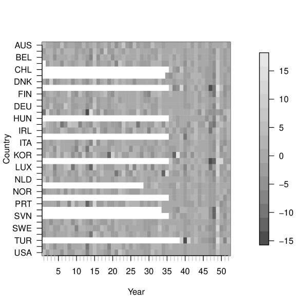
Figure 7: Heat plot (greyscale) of the differenced time series, where the initial white space indicates missing time series observations.

4.1 Finding a network to aid prediction

This section considers the case where we observe data up to $t=51$, and then wish to predict the values for each node at $t=52$. We begin by exploring ‘within-sample’ prediction at $t=51$, and identify a good network for prediction. We use randomly generated Erdős-Rényi graphs using the GNAR function seedToNet. To demonstrate this, the GNAR package contains the gdp data and a set of seed values, seed.nos so that the random graphs can be reproduced for use with the time series object gdpVTS here. R> net1 <- seedToNet(seed.no = seed.nos[1], nnodes = 35, graph.prob = 0.15) R> net2 <- seedToNet(seed.no = seed.nos[2], nnodes = 35, graph.prob = 0.15) R> layout(matrix(c(2, 1), 1, 2)) R> par(mar=c(0,1,0,1)) R> plot(net1, vertex.label = colnames(gdpVTS), vertex.size = 0) R> plot(net2, vertex.label = colnames(gdpVTS), vertex.size = 0)

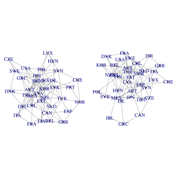
Figure 8: Erdős-Rényi random graphs constructed from the first two elements of the seed.nos variable with 35 nodes and connection probability 0.15.

Figure 8 shows two of these random graphs.

As well as investigating which network works best for prediction, we also need to identify the number of parameters in the GNAR model. Initial analysis of the autocorrelation function at each node indicated that a second-order autoregressive component should be sufficient, so GNAR models with orders up to $p=2$ were tested, and we included at most two neighbour sets at each time lag. The GNAR models are: GNAR$(1,[0])$, GNAR$(1,[1])$, GNAR$(2,[0,0])$, GNAR$(2,[1,0])$, GNAR$(2,[1,1])$, GNAR$(2,[2,0])$, GNAR$(2,[2,1])$, and GNAR$(2,[2,2])$, each fitted as individual-$\alpha$ and global-$\alpha$ GNAR models, giving sixteen models in total.

For the GDP example, we simulate 10,000 random un-directed networks, each with connection probability 0.15, and predict using the GNAR model with the orders above. Hence, this example requires significant computation time (about 90 minutes on a desktop PC), so only a segment of the analysis is included in the code below. For computational reasons, we first divide through by the standard deviation at each node so that we can model the residuals as having equal variances at each node. The function seedSim outputs the sum of squared differences between the prediction and original values, and we use this as our measure of prediction accuracy. R> gdpVTSn <- apply(gdpVTS, 2, function(x)x / sd(x[1:50], na.rm = TRUE)) R> alphas <- c(rep(1, 2), rep(2, 6)) R> betas <- list(c(0), c(1), c(0, 0), c(1, 0), c(1, 1), c(2, 0), c(2, 1), + c(2, 2)) R> seedSim <- function(seedNo, modelNo, globalalpha) + net1 <- seedToNet(seed.no = seedNo, nnodes = 35, graph.prob = 0.15) + gdpPred <- predict(GNARfit(vts = gdpVTSn[1:50, ], net = net1, + alphaOrder = alphas[modelNo], betaOrder = betas[[modelNo]], + globalalpha = globalalpha)) + return(sum((gdpPred - gdpVTSn[51, ])^2)) + R> seedSim(seedNo = seed.nos[1], modelNo = 1, globalalpha = TRUE) [1] 23.36913 R> seedSim(seed.nos[1], modelNo = 3, globalalpha = TRUE) [1] 11.50739 R> seedSim(seed.nos[1], modelNo = 3, globalalpha = FALSE) [1] 18.96766 Prediction error boxplots over simulations from all sixteen models and 10,000 random networks are shown in Figure 9 (accompanying code not shown due to significant computation time). The global-$\alpha$ model resulted in lower prediction error in general, so we use this version of the GNAR model. For GNAR$(1,[0])$ and GNAR$(2,[0,0])$, the first and third model in Figure 9 the “boxplots” are short horizontal lines as the results for each graph are identical, as no neighbour parameters are fitted.

Figure 9: Prediction error boxplots at $t=51$ over 10,000 randomly generated networks using seed.nos and different GNAR models, where ‘g-$\alpha$’ indicates a global-$\alpha$ GNAR model.

As the other global-$\alpha$ models are nested within it, we select the randomly generated graph that minimises the prediction error for global-$\alpha$ GNAR$(2,[2,2])$; this turns out to be the network generated from seed.nos[921]. R> net921 <- seedToNet(seed.no = seed.nos[921], nnodes = 35, + graph.prob = 0.15) R> layout(matrix(c(1), 1, 1)) R> plot(net921, vertex.label = colnames(gdpVTS), vertex.size = 0)

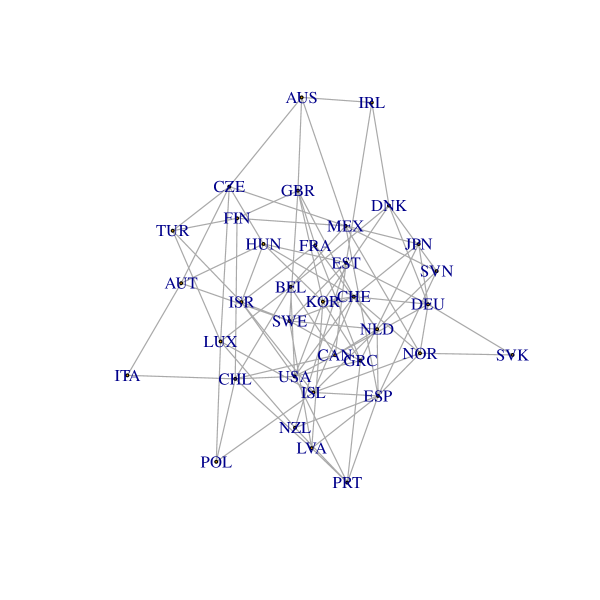
Figure 10: Randomly generated un-weighted and un-directed graph over the OECD countries that minimises the prediction error at $t=51$ using GNAR$(2,[2,2])$.

The network generated from seed.nos[921] is plotted in Figure 10, where all countries have at least two neighbours, with 97 edges in total. This “921” network was constructed with GDP prediction in mind, so we would not necessarily expect any interpretable structure in our found network (and presumably, there were other networks with not too dissimilar predictive power). However, the USA, Mexico and Canada are extremely well-connected with eight, eight and six edges, respectively. Sweden and Chile are also well-connected, with eight and seven edges, respectively. This might seem surprising, but, e.g., the McKinsey Global Institute MGI Connectedness Index, see McKinsey2016, ranks Sweden and Chile 18th and 45th respectively out of 139 countries, and each country is most connected within their regional bloc (Nordic and South America, respectively). Each of these edges, or subgraphs of the “921” network could be tested to find a sparser network with a similar predictive performance, but we continue with the full chosen network here.

Using this network, we can select the best GNAR order using the BIC. R> res <- rep(NA, 8) R> for(i in 1:8) + res[i] <- BIC(GNARfit(gdpVTSn[1:50, ], + net = seedToNet(seed.nos[921], nnodes = 35, graph.prob = 0.15), + alphaOrder = alphas[i], betaOrder = betas[[i]])) + R> order(res) [1] 6 3 4 7 8 5 1 2 R> sort(res) [1] -64.44811 -64.32155 -64.18751 -64.12683 -64.09656 -63.86919 [7] -60.67858 -60.54207 The model that minimised BIC in this case was the sixth model, GNAR$(2,[2,0])$, a model with two autoregressive parameters and network regression parameters on the first two neighbour sets at time lag one.

4.2 Results and comparisons

We use the previous section’s model to predict the values at $t=52$ and compare its prediction errors to those found using standard AR and VAR models. The GNAR predictions are found by fitting a GNAR$(2,[2,0])$ model with the chosen network (corresponding to seed.nos[921]) to data up to $t=51$, and then predicting values at $t=52$. We first normalise the series, and then compute the total squared error from the model fit. R> gdpVTSn2 <- apply(gdpVTS, 2, function(x)x / sd(x[1:51], na.rm = TRUE)) R> gdpFit <- GNARfit(gdpVTSn2[1:51,], net = net921, alphaOrder = 2, + betaOrder = c(2, 0)) R> summary(gdpFit) Call: lm(formula = yvec2   dmat2 + 0)

Residuals: Min 1Q Median 3Q Max -3.4806 -0.5491 -0.0121 0.5013 3.1208

Coefficients: Estimate Std. Error t value Pr(>|t|) dmat2alpha1 -0.41693 0.03154 -13.221 < 2e-16 *** dmat2beta1.1 -0.12662 0.05464 -2.317 0.0206 * dmat2beta1.2 0.28044 0.06233 4.500 7.4e-06 *** dmat2alpha2 -0.33282 0.02548 -13.064 < 2e-16 *** — Signif. codes: 0 ’***’ 0.001 ’**’ 0.01 ’*’ 0.05 ’.’ 0.1 ’ ’ 1

Residual standard error: 0.8926 on 1332 degrees of freedom (23 observations deleted due to missingness) Multiple R-squared: 0.1859, Adjusted R-squared: 0.1834 F-statistic: 76.02 on 4 and 1332 DF, p-value: < 2.2e-16

GNAR BIC: -62.86003 R> sum((predict(gdpFit) - gdpVTSn2[52, ])^2) [1] 5.737203 The fitted parameters of this GNAR model were $\hat{\alpha}_{1}\simeq-0.42,\hat{\beta}_{1,1}\simeq-0.13,\hat{\beta}_{1,2}\simeq 0.28,$ and $\hat{\alpha}_{2}\simeq-0.33$.

We compared our methods with results from fitting an AR model individually to each node using the forecast.ar() and auto.arima() functions from version 8.0 of the CRAN forecast package (hyndman17:forecast), for further details see Hyndman2008. Due to our autocorrelation analysis from Section 4.1 we set the maximum AR order for each of the 35 individual models to be $p=2$. Conditional on this, the actual order selected was chosen using the BIC. R> library("forecast") R> arforecast <- apply(gdpVTSn2[1:51, ], 2, function(x) + forecast(auto.arima(x[!is.na(x)], d = 0, D = 0, max.p = 2, max.q = 0, + max.P = 0, max.Q = 0, stationary = TRUE, seasonal = FALSE, ic = "bic", + allowmean = FALSE, allowdrift = FALSE, trace = FALSE), h = 1)$mean+$) R> sum((arforecast - gdpVTSn2[52, ])^2) [1] 8.065491 Our VAR comparison was calculated using version 1.5–2 of the CRAN package vars, Pfaff2008. The missing values at the beginning of the series cannot be handled with current software, so are set to zero. The number of parameters in a zero-mean VAR($p$) model is of order $pN^{2}$. In this particular example, the dimension of the observation data matrix is $T\times N$, with $T<2N$, so only a first-order VAR can be fitted. We fit the model using the VAR function and then use the restrict function to reduce dimensionality further, by setting to zero any coefficient whose associated absolute $t$-statistic value is less than two. R> library("vars") R> gdpVTSn2.0 <- gdpVTSn2 R> gdpVTSn2.0[is.na(gdpVTSn2.0)] <- 0 R> varforecast <- predict(restrict(VAR(gdpVTSn2.0[1:51, ], p = 1, + type = "none")), n.ahead = 1)

This results in forecast vectors for each node, so we extract the point forecast (the first element of the forecast vectors) and compute the prediction error as follows R> getfcst <- function(x)return(x[1]) R> varforecastpt <- unlist(lapply(varforecast$fcst,getfcst))R>sum((varforecastpt-gdpVTSn2.0[52,]){}^2)[1]26.19805\text{Table 1Table 11Table 1Model\# ParametersPrediction errorGNAR(2,[2,0])45.7Individual AR(2)388.1VAR(1)19926.21Estimatedpredictionerro}$