Arbitrary optical wave evolution with Fourier transforms and phase masks

Abstract

A large number of applications in classical and quantum photonics require the capability of implementing arbitrary linear unitary transformations on a set of optical modes. In a seminal work by Reck et al. (Reck et al., 1994) it was shown how to build such multiport universal interferometers with a mesh of beam splitters and phase shifters, and this design became the basis for most experimental implementations in the last decades. However, the design of Reck et al. is difficult to scale up to a large number of modes, which would be required for many applications. Here we present a constructive proof that it is possible to realize a multiport universal interferometer on $N$ modes with a succession of $6N$ Fourier transforms and $6N+1$ phase masks, for any even integer $N$. Furthermore, we provide an algorithm to find the correct succesion of Fourier transforms and phase masks to realize a given arbitrary unitary transformation. Since Fourier transforms and phase masks are routinely implemented in several optical setups and they do not suffer from the scalability issues associated with building extensive meshes of beam splitters, we believe that our design can be useful for many applications in photonics.

Introduction.— The ability to arbitrarily transform an optical mode has applications spanning communications, imaging, and information processing. Such a transformation that is lossless and linear is described by a unitary matrix $U$, mapping a basis of $N$ input modes onto a basis of $N$ output modes. Since any such matrix has $N^{2}$ free parameters, a method for its implementation must have at least $N^{2}$ controllable parameters, which is an experimentally challenging scaling. One implementation method is based on optical Fourier transforms (FT) (Morizur et al., 2010; Armstrong et al., 2012; Labroille et al., 2014). In this paper, we show that only $N^{2}$ controllable parameters are needed to implement an arbitrary unitary transformation on $N$ modes using FTs. What is more, we introduce a deterministic algorithm to design an arbitrary unitary transformation based on this method.

General variable control of modal unitary transformations will have applications across optics. For example, in fiber optic communications, spatial multiplexing will require transforming between an array of Gaussian profile modes from, say, a ribbon of single-mode fibers to the non-Gaussian spatial modes of one multimode fiber (Bozinovic et al., 2013). Routing of optical channels requires a reconfigurable network, described by a unitary (Zhuang et al., 2015; Pérez et al., 2017). Information processing with optical networks takes advantage of the ultra-low latency and ultra-high clock speed of photonic waveguides. Capitalizing on this allows for one to, for instance, concatenate two unitary transformations to quickly multiply two matrices, a key ingredient in a neural network (Shen et al., 2017; Steinbrecher et al., 2019). Another area of application, imaging, is, at its heart, a unitary spatial transformation. General unitary transformations would enable novel imaging functionalities, such as cancelling the optical scattering that inhibits imaging through human tissue (Popoff et al., 2010a, b). Image processing, such as noise reduction, sharpening, or compression, could be done on the field itself, rather than the intensity recorded by the sensor (Silva et al., 2014). Turning to the area of quantum information, a generalization of the $N=2$ qubit is a photon in a superposition of $N$ modes, a qudit (Schaeff et al., 2015; Larocque et al., 2017). In quantum cryptography, a protocol that uses qudits (and unitaries on them) rather than qubits improves the robustness to noise (Bouchard et al., 2018). Quantum computing logic gates, such as the controlled-NOT gate, can be implemented using unitary transformations on photonic waveguide modes (Politi et al., 2008). Moreover, random walks in waveguide-network transformations simulate a variety of quantum systems (Harris et al., 2017), such as molecules (Peruzzo et al., 2010). The problem of sampling the output probability distribution when multiple photons traverse such networks is hard to simulate in a classical computer and hence it may be a viable path to achieve quantum supremacy with photonic devices, as proved in (Aaronson and Arkhipov, 2013). The underlying reason is that sampling the bosonic statistics of the output photons is linked to the problemn of estimating the permanent of a large unitary matrix (Broome et al., 2013; Crespi et al., 2013; Spring et al., 2013; Tillmann et al., 2013), which is #P-hard (Valiant, 1979). These applications motivate why the field is spending considerable effort to develop controllable unitary transformations.

We now briefly outline these efforts and methods. While the first methods to create arbitrary transformations were developed during early radio and microwave engineering, Reck et al. introduced them to optics in a seminal paper in 1994 (Reck et al., 1994). One of the simplest tools available in optics is a phase shifter. However, by themselves modal phase-shifters are insufficient to build a general unitary transformation. In addition, one must use mode-mixing elements such as beamsplitters. Reck et al. gave a prescription to implement any chosen unitary on an array of beam modes by using a triangle-shaped lattice of variable-reflectivity beamsplitters interleaved with phase shifters. However, the complexity of this method meant it was not demonstrated until an integrated optical implementation over twenty years later (Carolan et al., 2015). Soon after, a more compact square lattice of beamsplitters and phase shifters was proposed and implemented by Clements et al. (Clements et al., 2016). Since the first implementation, a range of integrated optical platforms have hosted proof-of-principle applications of these lattices (Crespi et al., 2016; Mennea et al., 2018; Ribeiro et al., 2016). However, the fabrication and control complexity associated with this method has, so far, limited demonstrations of arbitrary unitaries to $N=6$ waveguides (Carolan et al., 2015).

Before these integrated optical implementations, a different type of mixer was proposed and implemented, a lens or curved mirror. The latter elements enact an approximate Fourier transform of the spatial field-distribution (Goodman, 2005). Using these, a unitary is decomposed into a series of FTs interleaved with phase-shifters (Morizur et al., 2010; Armstrong et al., 2012; Labroille et al., 2014), as shown in Fig. 1. The phase shifters are varied to implement a given unitary, whereas the FTs do not change. An SLM of $N$ pixels per side will inherently contain the $N^{2}$ control parameters required to implement a unitary for a spatial mode that varies along a row of pixels. Moreover, since they are based on television technology (e.g., 4K resolution) they currently have up to $N^{2}=8$ million pixels. A series of experiments using multiple reflections from a curved mirror and a phase-shifting spatial light modulator array (SLM) successfully demonstrated a variety of unitary transformations (Labroille et al., 2014; Morizur et al., 2010). Fourier transforms can also be realized for other types of modes, for instance waveguides modes and spectral temporal modes, in an efficient manner (Lim and Rhee, 2011; Lu et al., 2018; Lukens and Lougovski, 2017). The FT method is the focus of this paper.

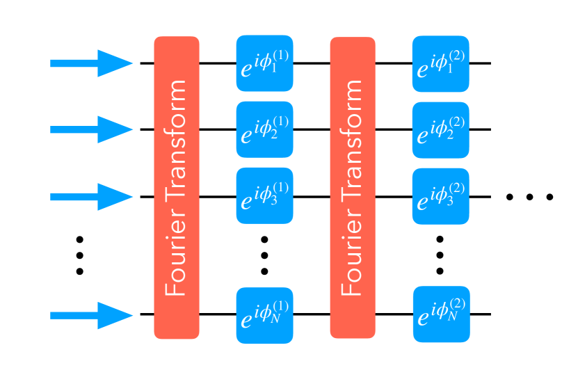
Figure 1: In this work we show that any linear unitary transformation between $N$ channels can be implemented by means of a succession of $6N+1$ phase masks (diagonal operators) and $6N$ Fourier transforms.

In particular, we give a deterministic algorithm to find the requisite phase-shifts in the FT method. Rather than using the full continuous FT, we use the discrete Fourier transform (DFT) since it is more amenable to matrix algebra. While there is an existence proof showing that a unitary could be decomposed into a sequence of FTs alternating with phase-shifters (Borevich and Krupetskii, 1981), there is no prescription for doing so with a sequence of realizable length. In (Schmid et al., 2000), a method was found to decompose an arbitrary matrix as a sequence of Fourier transforms and non-unitary diagonal matrices. However, their method is not adequate for linear optical setups, since their prescription makes use of non-unitary diagonal masks. Furthermore, the length scales as $N^{3}$, which is very far from the optimal scaling $L\sim N$. That said, an optimization algorithm to determine these phase shifts, ‘wavefront matching’, was recently introduced and experimentally validated (Fontaine et al., 2019). While practical, iterative optimization has a number of drawbacks for the FT method: 1. There is no guarantee of a solution nor its global optimality 2. It does not prescribe the design parameters, e.g., the required number of required FT-phase shift iterations, resolution (i.e., SLM pixel size), and range (i.e., number of pixels). Thus, it is unknown what is required to achieve a unitary of a given dimension, level of optical loss, or amount of error. 3. Relative to the Reck et al.’s deterministic algorithm, it is computationally slow. 4. It does not provide physical insight into how to develop improved methods. Consequently, there is a need for the deterministic algorithm we introduce here.

In the first section, we map the Clements et al. lattice onto the FT method. That is, we decompose a layer of beamsplitters in the lattice into a short sequence of FTs and fixed phase shifts. We use this to adapt their deterministic algorithm to find the requisite variable phase shifts in the FT method. Consequently, we give an explicit prescription for how to design a unitary transformation with the FT method. While the FT is often numerically computed using the DFT, in the second section, we show that the DFT can also directly occur in optical systems. We show that, for example, modal propagation in a box waveguide is described by a DFT. In the appendix, we give a detailed derivation of our FT method decomposition. More broadly, the FT method is not restricted to optics, being directly applicable to many other setups such as neutral atoms in optical traps or phonon modes in ion chains.

Decomposition method.— Any lossless, noiseless, linear transformation on a closed system of $N$ optical modes is described by a unitary matrix $U\in\mathcal{U}_{N}(\mathbb{C})$. Reck et al. showed that any unitary transformation between optical modes can be implemented as a lattice of beam splitters (Reck et al., 1994). Such a lattice is also known as a multiport interferometer. A beam splitter is an optical element that mixes two modes $i$ and $j$ according to unitary matrix $T(\theta,\phi)\in\mathcal{U}_{N}(\mathbb{C})$ parametrized by two angles $\phi,\theta\in[0,2\pi)$

$$\begin{pmatrix}\left[T(\theta,\phi)\right]_{ii}&\left[T(\theta,\phi)\right]_{ij}\\ \left[T(\theta,\phi)\right]_{ji}&\left[T(\theta,\phi)\right]_{jj}\end{pmatrix}:=\begin{pmatrix}e^{i\phi}cos(\theta)&-sin(\theta)\\ e^{i\phi}sin(\theta)&cos(\theta)\end{pmatrix}.$$ (1)

It acts as the identity matrix on all the other channels. An arbitrary beam splitter $T_{ij}(\theta,\phi)$ can be factorized in the following way

$$\begin{pmatrix}e^{i\phi}cos(\theta)&-sin(\theta)\\ e^{i\phi}sin(\theta)&cos(\theta)\end{pmatrix}=X\begin{pmatrix}e^{i\theta}&0\\ 0&1\end{pmatrix}X\begin{pmatrix}e^{i\phi}&0\\ 0&1\end{pmatrix},$$ (2)

where $X$ represents a 50-50 beam splitter, i.e., $X:=\frac{1}{\sqrt{2}}\begin{pmatrix}1&1\\ 1&-1\end{pmatrix}$. Hence, one only needs controllable phase shifters and fixed 50-50 beam splitters to build the lattice of beam splitters designed by Reck et al.

Instead of a beamsplitter-based method, here we investigate a factorization method based on Fourier transforms. As a starting point,we consider the Discrete Fourier Transform (DFT), whose action is described by a unitary matrix whose elements are given by $F_{jk}=\frac{1}{\sqrt{N}}e^{i2\pi jk/N}$. Our design is built as a succession of Fourier transforms and phase masks:

$$U=D^{(0)}\prod_{i=1}^{L}FD^{(i)}.$$ (3)

The phase masks $\left\{D^{(i)}\right\}_{i\in\left\{0,..,L\right\}}$ are the only element in this setup that we can control. Each phase mask on $N$ modes is described by a diagonal matrix parametrized by $N$ angles, $D_{jk}^{(i)}=e^{i\alpha_{j}^{(i)}}\delta_{jk}$. Thus, it is clear that one needs at least $N$ of them to simulate an arbitrary multiport interferometer such as the Reck scheme.

We present a way to find a decomposition of an arbitrary unitary matrix in the form displayed in Eq.(3), consisting of $L+1=6N+1$ unitary diagonal matrices and $6N$ DFT matrices. In our factorization method, rather than the Reck et al. method we start from the decomposition in beam splitters given by Clements et al. in (Clements et al., 2016). Their design consists of a mesh of beam splitters arranged in $N$ consecutive layers. The composition of the action of all the beam splitters in the mesh has the following form

$$U =D\prod_{i=1}^{N/2}\prod_{k=1}^{N/2-1}T_{2k}(\chi_{k}^{(i)},\eta_{k}^{(i)})\prod_{j=1}^{N/2}T_{2j-1}(\theta_{j}^{(i)},\phi_{j}^{(i)}),$$ (4)

where $T_{j}(\theta,\phi)$ is a beam splitter mixing channels $j$ and $j+1$. As pointed out above in Eq.(2), any beam splitter can be implemented with two 50-50 beam splitters and two phase shifters. Therefore, the design proposed in (Clements et al., 2016) can be understood as a succession of layers of 50-50 beam splitters and phase masks. The procedure to translate the lattice of beam splitters into a composition of phase masks and DFT’s is schematically depicted in Figure (2). In a nutshell, our decomposition builds on this by factoring each layer of 50-50 beam splitters in the mesh as a product of Fourier transforms and phase masks. Since the proof is constructive, it automatically gives a method to find the parameters in terms of $U$. Our decomposition needs only $N^{2}$ free controllable parameters, which is optimal. However, an improvement by a constant factor in the optical length (i.e. the total number of phase masks required) may still be possible.

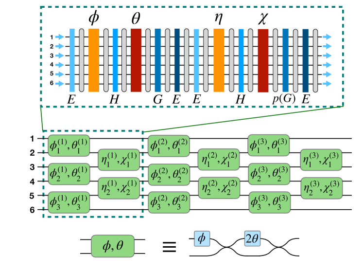
Figure 2: Any unitary matrix can be realized by a mesh of beam splitters, as described in (Clements et al., 2016). Our decomposition method is based on replacing each layer of beam splitters by a succession of discrete Fourier transforms and phase masks, as schematically depicted here at the top. Each layer of beam splitters requires six Fourier transforms (grey rounded rectangles) and 6 phase-mask diagonal matrices (coloured rectangles). Only two diagonal matrices per layer (red and yellow rectangles) depend on the unitary matrix that is being implemented, while the rest (blue rectangles) are fixed. The general expression for the phase masks is given in Eqs(6,7,8).

Consider that we want to decompose a given unitary matrix $U$. In the decomposition displayed in Eq.(4), each term of the form $\prod_{k=1}^{N/2-1}T_{2k}(\chi_{k}^{(i)},\eta_{k}^{(i)})$ represents a layer of beam splitters connecting each even channel $2j$ with the odd channel $2j+1\ (\mathrm{mod}\ N)$, whereas each term $\prod_{j=1}^{N/2}T_{2j-1}(\theta_{j}^{(i)},\phi_{j}^{(i)})$ represents a layer of beam splitters connecting each even channel $2j$ with the odd channel $2j-1\ (\mathrm{mod}\ N)$. It will turn out to be more convenient for us if we relabel the indices as $\left\{0,1,2,3,...\right\}\rightarrow\left\{0,\frac{N}{2},1,\frac{N}{2}+1,...\right\}$. Then, we can see that $U$ can also be decomposed as a succession of layers of beam splitters such that in the odd layers each beam splitter connects each channel $j\in\left\{N/2,...,N-1\right\}$ with the channel $j-N/2$, whereas in the even layers each beam splitter connects the channel $j\in\left\{N/2,...,N-1\right\}$ with the channel $j-N/2+1\ (\mathrm{mod}\ \frac{N}{2})$.

On the one hand, the odd layers can be written as $X\Xi{}_{1}^{(i)}X\Xi_{2}^{(i)}$, where $\Xi_{1}^{(i)},\Xi_{2}^{(i)}$ are diagonal matrices. On the other hand, the even layers have the same structure as the odd layers after a cyclic shift of the first half of the channels. In other words, each even layer of beam splitters can be expressed as $P^{T}X\Omega_{1}^{(i)}X\Omega_{2}^{(i)}P$, where $\Omega_{1}^{(i)},\Omega_{2}^{(i)}$ are also diagonal matrices, and $P$ is just the permutation matrix given by

$$P_{jk}:=\begin{cases}1&k=j+1\,\mod\left(\frac{N}{2}\right),\,j\leq\frac{N}{2}-1\\ 1&k=j,\,j>\frac{N}{2}-1\\ 0&\textrm{{otherwise}}.\end{cases}$$ (5)

Then, it follows that any unitary matrix admits the following decomposition

$$U=D\prod_{i=1}^{N/2}\prod_{k=1}^{N/2-1}P^{T}X\Omega_{1}^{(i)}X\Omega_{2}^{(i)}P\prod_{j=1}^{N/2}X\Xi_{1}^{(i)}X\Xi_{2}^{(i)}.$$

At this point, we only have to find how to decompose the matrices X and $P$ as a product of phase masks and Fourier transforms. In order to do this, we will find how to factorize them in products of circulant and diagonal matrices. A circulant matrix is a matrix such that each row is obtained by applying a cyclic shift by one slot to the right to the previous row. Since any circulant matrix is diagonalized by the DFT matrix $F$, a product of circulant and diagonal matrices can always be re-expressed as a product involving only $F$, $F^{\dagger}$ and diagonal matrices.

Let us define the diagonal matrix $G:=\begin{pmatrix}I&0\\ 0&iI\end{pmatrix}$ and the circulant matrix $Y:=\frac{1}{\sqrt{2}}\begin{pmatrix}I&-iI\\ -iI&1\end{pmatrix}$. First, we note that $X=GYG$. Second, we observe that the permutation matrix $P$ can be factorized as a product of three circulant matrices and four diagonal matrices in the following way

$$P=\frac{1}{\sqrt{2}}X\begin{pmatrix}C+I&C-I\\ C-I&C+I\end{pmatrix}X,$$

where $C$ is the cyclic shift matrix $C=\delta_{j,j+1\ (\mathrm{mod}\ N/2)}$ of size $\frac{N}{2}\times\frac{N}{2}$. Therefore, we have shown how to decompose any unitary matrix $U$ as a product of diagonal and circulant matrices. If then we diagonalize the circulant matrices, we immediately obtain a factorization of $U$ involving only $F$, $F^{\dagger}$ and diagonal matrices. But the inverse of the DFT matrix is just $F^{\dagger}=\Pi F=F\Pi$, where $\Pi$ is the following permutation matrix

$$\Pi_{jk}=\begin{cases}1&j=k=0\\ 1&j=N-k\\ 0&\textrm{otherwise}.\end{cases}$$

Since $\Pi D\Pi$ is diagonal whenever $D$ is diagonal, we can decompose $U$ using only $F$ and diagonal matrices.

In the end, diagonalizing all the circulant matrices we obtain the following expression

$$U=DG\left[\prod_{i=1}^{N/2}B^{(i)}A^{(i)}\right]G{}^{\dagger},$$

where the terms $B^{(i)},A^{(i)}$ are given by

$$B^{(i)} =\left\{E,p\left(G\right),H,\Gamma(\chi^{(i)}),E,p\left(G\Gamma(\eta^{(i)})\right)\right\}_{F},$$ (6)

$$A^{(i)} =\left\{E,G,H,p\left(\Gamma(\theta^{(i)})\right),E,G\Gamma(\phi^{(i)})\right\}_{F},$$ (7)

where we made use of the notation

$$\left\{D_{1},...,D_{N}\right\}_{F}:=\prod_{i=1}^{N}FD_{i}.$$

The diagonal matrices $E,H$ are defined as

$$E_{jj}=\frac{1}{\sqrt{2}}\left[1-i\left(-1\right)^{j}\right],$$

$$H_{jj}=\frac{1}{2}\left[1-(-1)^{j}\right]+\frac{1}{2}\left[1+(-1)^{j}\right]e^{i2\pi j/N},$$

and the diagonal matrix $\Gamma(\mathbf{v})$ is defined as a function of a real vector $\mathbf{v}\in\mathbb{R}^{N/2}$:

$$\begin{array}[]{c}\left[\Gamma(\mathbf{v})\right]_{jj}:=\begin{cases}e^{iv_{j}}&j<\frac{N}{2}-1\\ i&j\geq\frac{N}{2}-1\end{cases}.\end{array}$$ (8)

Finally, $p:\mathcal{U}_{N}\rightarrow\mathcal{U}_{N}$ is just the map $p(U):=\Pi U\Pi$. Note that when applied on a diagonal matrix, it just inverts the order of the diagonal entries after the first one: $p\left(diag(a_{0},a_{1},...,a_{N-1})\right)=diag(a_{0},a_{N-1},...,a_{1}).$

We now summarize the procedure to create any unitary transformation $U$ using phase-masks and DFTs. This procedure is based on using Eqs.(6,7) to express a unitary matrix according to the factorization in Eq.(3). First, we permute the channels of the unitary transformation as described in the proof, which corresponds to computing the matrix $U_{P}=P^{T}UP$, with $P$ being the permutation matrix defined in Eq.(5). Then, we find the decomposition of $U_{P}$ as a lattice of beam splitters by the procedure described in Clements et al. (Clements et al., 2016). That is, we find the parameters $\left\{(\chi^{(i)},\eta^{(i)},\theta^{(i)},\phi^{(i)})\right\}_{i=\left\{0,...,N/2-1\right\}}$ for each lattice layer $i$ such that $U_{P}$ is factorized in the form given by Eq.(4). The procedure for finding these parameters is explained in (Clements et al., 2016), but the general idea is to null, one by one, all the off-diagonal elements of $U_{P}$ by means of an appropriate succession of beam splitters. We then apply these parameters $\left\{(\chi^{(i)},\eta^{(i)},\theta^{(i)},\phi^{(i)})\right\}_{i}$ as phase masks along with other fixed phase masks, all interleaved with DFTs, to replace layer $i$. In Fig. 2, we indicate all seven different diagonal matrices (e.g., phase masks), $E,$ $H$, $G$, $p(G)$, and $\Gamma(\mathbf{v})$ (labelled by the value of $\mathrm{\mathbf{v}}=\chi,\eta,\theta,$ and $\phi$), at the location of their application within one layer $i$ of our method. All the control parameters are contained in the diagonal matrices $\Gamma(\mathbf{v})$, whereas the rest of the diagonal matrices are fixed. In the end, the computation of all the diagonal matrices is quite efficient, as it only requires $\mathcal{O}(N^{2})$ operations. In summary, applying the structure in Fig. 2 in place of each the $N/2$ beamsplitter lattice layers results in an implementation of an arbitrary unitary using only phase-masks and Fourier transforms.

Physical Implementation of the DFT.— Our decomposition method requires the capability to optically perform the DFT. Although the standard continuous Fourier transform is routinely approximately performed in optical experiments with several setups, such as lenses (Cutrona et al., 1960), curved mirrors (Nikolov, 1982), or arrayed waveguide gratings(Lim and Rhee, 2011), implementing the DFT by optical means is not a trivial problem. In waveguide systems a ’star coupler’, sometimes called a $N\times N$ symmetric multiport or splitter, is sometimes said to perform a DFT-like operation in that any given input mode is transformed to a flat distribution of output modes. That is, the unitary matrix that describes the star coupler matches the magnitudes of the DFT matrix, $|F_{jk}|$, but the phases will likely be incorrect. Since setting the magnitude only removes half of the free parameters in a unitary matrix, $N^{2}/2$ parameters still must be adjusted to match a DFT. This cannot be accomplished by sandwiching the star coupler between two phase-masks since they only have $2N$ parameters together. Consequently, to implement our method there is a need for an optical DFT in waveguide systems.

Here we discuss one possible procedure to optically compute the DFT that is based on the phenomenon of self-imaging inside a multimode waveguide (Bachmann et al., 1994). The idea of using multimode intereference (MMI) couplers to realize the DFT is not new, and it was first proposed in (Zhou, 2010). However, their prescription uses an $2N\times 2N$ MMI coupler to output two copies of the $N$ dimensional DFT on half of the input modes, which is not amenable to our goal. Here we describe a method to implement the DFT on $N$ modes with an $N\times N$ MMI coupler, using all $N$ modes. As it only needs a planar waveguide and phase shifts, we believe that our proposal could be easily scaled to a large number of modes. Furthermore, it can be generalized to many other setups, such as neutral atoms in optical traps.

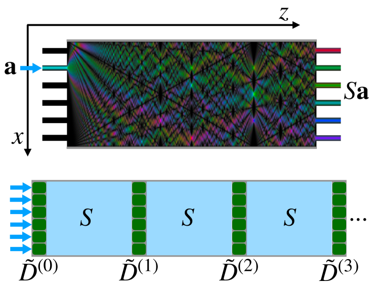
Figure 3: Free propagation inside a multimode waveguide can be used to realize the DFT (in this case, a $6\times 6$ DFT). When a wavepacket is injected in the waveguide, the output at a particular value of the propagation length is a superposition of $N$ copies of the wavepacket weighted with complex phases. It can be shown that he output field is nothing else than the DFT of the input field modulo phase masks and permutation of the indices of the input and output modes. Therefore, a combination of free propagation inside multimode waveguides and controllable phase masks is enough to realize arbitrary unitary transformations.

Consider a planar waveguide of width $w$ and index of refraction $n$. We parametrize the transversal coordinate as $x$ and the longitudinal coordinate as $z$. Let us assume hard wall boundary conditions, so that it supports guided modes of the form $\psi_{n}(x)=\sin(k_{xn}x)$, where $k_{xn}=\frac{\pi(n+1)}{w}$. Furthermore, let us assume that the length of the waveguide is much larger than its width. Then, in the paraxial limit we can approximate $k_{zj}=nk_{0}-k_{xj}^{2}/2nk_{0}$, where $k_{0}:=\frac{2\pi}{\lambda}$.

Consider now that at $z=0$ we input a wavepacket $f(x-x_{j}^{in})$ centered at $x_{j}^{in}$. For simplicity, let us assume that $x_{j}:=\left(j+\frac{1}{2}\right)\frac{w}{N}$, for some integer $j\in\left\{0,...,N-1\right\}$. This defines a vector basis for our target DFT matrix in terms of $N$ wavepacket modes. Under the assumptions listed above, it has been shown in (Bachmann et al., 1994) that when the propagation length is set to be equal to $z_{N}=\frac{2nk_{0}}{\pi N}w^{2}$, the output field is given by

$$E_{out}(x)=\frac{1}{\sqrt{N}}\sum_{k=0}^{N-1}e^{i\chi_{jk}}f\left(x-x_{k}^{out}\right).$$ (9)

In other words, the output field is a superposition of $N$ repetitions of the input wavepacket at $N$ distinct positions and weighted by complex phases. The wavepackets $f\left(x-x_{k}^{out}\right)$ define the output mode basis, where $x_{j}^{out}=\left(N-j-\frac{1}{2}\right)\frac{w}{N}$, and the complex phase weights compose a unitary matrix, $S_{jk}:=\frac{1}{\sqrt{N}}e^{i\chi_{jk}}$. In (Bachmann et al., 1994) these weights were shown to be

$$S_{jk}=\begin{cases}\frac{1}{\sqrt{N}}e^{i\frac{\pi}{4N}\left(k-j\right)\left(2N-k+j\right)+i\zeta_{0}}&\textrm{{if }}j+k\textrm{ is even}\\ \frac{1}{\sqrt{N}}e^{i\frac{\pi}{4N}\left(k+j+1\right)\left(2N-k-j-1\right)+i\zeta_{0}}&\textrm{{if }}j+k\textrm{ is odd,}\end{cases}$$ (10)

where $\zeta_{0}:=-k_{0}z_{N}-\frac{\pi}{4}$. It is straightforward to check that in fact the unitary matrix $S$ is nothing else than the DFT matrix left and right multiplied by a diagonal matrix and a permutation matrix

$$S=R^{T}\Theta F\Theta R,$$ (11)

where the permutation matrix $R$ and the diagonal matrix $\Theta$ are given by

$$R_{jk}:=\begin{cases}1&j\leq N/2\textrm{ and }2j-k-1=0\\ 1&j>N/2\textrm{ and }2j+k-2N-2=0\\ 0&\textrm{otherwise}\end{cases},$$

$$\Theta_{jj}:=e^{i\frac{\pi}{4N}\left\lfloor\frac{j+1}{2}\right\rfloor^{2}-i\frac{\zeta_{0}}{2}+i\pi\left\lfloor\frac{j+1}{2}\right\rfloor}.$$

Eq.(11) implies a possible optical implementation of the DFT. The setup would consist of a planar multimode waveguide with length $z_{N}$ coupled to $N$ input channels and $N$ output channels as in figure (3). For an input field $E_{in}=\sum_{j=0}^{N-1}a_{j}f\left(x-x_{j}^{in}\right)$, the output field is $E_{out}=\sum_{j=0}^{N-1}\tilde{a}_{j}f\left(x-x_{j}^{out}\right)$, where the coefficients of the output are related to the coefficients of the input by $\tilde{\mathbf{a}}=S\mathbf{a}$.

Consider that we want to implement an arbitrary unitary matrix $U$ directly using such an MMI. Let us define the unitary matrix $U_{R}=RUR^{T}$. We can use the previous results to find its factorization, $U_{R}=D^{(0)}\prod_{i=1}^{L}FD^{(i)}$. Then, writing $F$ in terms of $S$ using Eq.(11), the unitary matrix $U$ can be factorized as $U=\tilde{D}^{(0)}\prod_{i=1}^{L}S\tilde{D}^{(i)}$, where we have defined the new diagonal matrices $\tilde{D}^{(0)}:=R^{T}D^{(0)}\Theta^{*}R$, $\tilde{D}^{(i)}:=\Theta^{*}R^{T}D^{(i)}R\Theta^{*},\,i=1,...,L-1$, and $\tilde{D}^{(L)}:=\Theta^{*}R^{T}D^{(L)}R$. Note that all matrices $\tilde{D}^{(i)}$ are indeed diagonal matrices, since $R$ is just a permutation matrix and $\Theta$ is also diagonal. In summary, to use such an MMI in place of an exact DFT one simply needs to modify the $L+1=6N+1$ phase-masks in our method.

This idea is not limited to optical modes in multimode waveguides. In fact, any physical system with confined modes of the form $\psi_{n}(x)=\sin(k_{xn}x)$ and a parabolic dispersion relation $E_{j}=\frac{k_{j}^{2}}{2m}$ can be used to realize the DFT. In this case, instead of propagating modes in a waveguide we consider a wavefunction that evolves inside a rectangular well according to the Schrödinger equation. We start with an input field of the form $\varphi(x,t=0)=\sum_{j=1}^{N}a_{j}\phi\left(x-x_{N-j+1}^{in}\right)$. Now, the state at any time is given by $\varphi(x,t)=\sum_{n}c_{n}e^{iE_{j}t}\psi_{n}(x)$. For free propagation, the dispersion relation is parabolic. Consequentially, all the mathematical expressions are formally equivalent to the ones that describe multimode interference in a waveguide. In particular, one could apply this protocol to neutral atoms confined in an optical trap.

Conclusion.— We have given an explicit, analytical, and deterministic procedure to design an implementation of an arbitrary unitary transformation of dimension $N$ using only discrete Fourier transforms and controllable phase-masks. The number of control parameters is the minimum possible, $N^{2}$. For mode sorting or multiplexing, where the global phase of each output state is irrelevant, the required number of DFT-phase-mask layers needed is $6N$. One additional phase-mask is required for a completely arbitrary unitary. Thus, the scaling of the number of layers with the dimension is linear and is optimal, up to an overall factor. We have also prescribed the first practical method to implement a DFT in integrated optics and even in systems outside optics, such as ion traps. The unitary matrix factorization we give could also be useful in quantum computation theory for decomposing quantum algorithms in terms of just two types of operations, the quantum Fourier transform and diagonal operators. We expect these results to be useful in a variety of classical and quantum information applications in photonics using various optical degrees of freedom including frequency-time, orbital angular momentum, and position-momentum.

References

- Reck et al. (1994) M. Reck, A. Zeilinger, H. J. Bernstein, and P. Bertani, Physical Review Letters 73, 58 (1994).
- Morizur et al. (2010) J.-F. Morizur, L. Nicholls, P. Jian, S. Armstrong, N. Treps, B. Hage, M. Hsu, W. Bowen, J. Janousek, and H.-A. Bachor, Journal of the Optical Society of America A 27, 2524 (2010).
- Armstrong et al. (2012) S. Armstrong, J.-F. Morizur, J. Janousek, B. Hage, N. Treps, P. K. Lam, and H.-A. Bachor, Nature Communications 3, 1026 (2012).
- Labroille et al. (2014) G. Labroille, B. Denolle, P. Jian, N. Treps, and J.-F. Morizur, , 9 (2014).
- Bozinovic et al. (2013) N. Bozinovic, Y. Yue, Y. Ren, M. Tur, P. Kristensen, H. Huang, A. Willner, and S. Ramachandran, Science 340, 1545 (2013).
- Zhuang et al. (2015) L. Zhuang, C. G. H. Roeloffzen, M. Hoekman, K.-J. Boller, and A. J. Lowery, Optica 2, 854 (2015).
- Pérez et al. (2017) D. Pérez, I. Gasulla, L. Crudgington, D. J. Thomson, A. Z. Khokhar, K. Li, W. Cao, G. Z. Mashanovich, and J. Capmany, Nature Communications 8, 636 (2017).
- Shen et al. (2017) Y. Shen, N. C. Harris, S. Skirlo, M. Prabhu, T. Baehr-Jones, M. Hochberg, X. Sun, S. Zhao, H. Larochelle, D. Englund, and M. Soljacic, Nature Photonics 11, 441 (2017).
- Steinbrecher et al. (2019) G. R. Steinbrecher, J. P. Olson, D. Englund, and J. Carolan, npj Quantum Information 5, 60 (2019).
- Popoff et al. (2010a) S. Popoff, G. Lerosey, R. Carminati, M. Fink, A. Boccara, and S. Gigan, Physical review letters 104, 100601 (2010a).
- Popoff et al. (2010b) S. Popoff, G. Lerosey, M. Fink, A. C. Boccara, and S. Gigan, Nature communications 1, 81 (2010b).
- Silva et al. (2014) A. Silva, F. Monticone, G. Castaldi, V. Galdi, A. Alù, and N. Engheta, Science 343, 160 (2014).
- Schaeff et al. (2015) C. Schaeff, R. Polster, M. Huber, S. Ramelow, and A. Zeilinger, Optica 2, 523 (2015).
- Larocque et al. (2017) H. Larocque, J. Gagnon-Bischoff, D. Mortimer, Y. Zhang, F. Bouchard, J. Upham, V. Grillo, R. W. Boyd, and E. Karimi, Opt. Express 25, 19832 (2017).
- Bouchard et al. (2018) F. Bouchard, K. Heshami, D. England, R. Fickler, R. W. Boyd, B.-G. Englert, L. L. Sánchez-Soto, and E. Karimi, Quantum 2, 111 (2018).
- Politi et al. (2008) A. Politi, M. J. Cryan, J. G. Rarity, S. Yu, and J. L. O’Brien, Science 320, 646 (2008).
- Harris et al. (2017) N. C. Harris, G. R. Steinbrecher, M. Prabhu, Y. Lahini, J. Mower, D. Bunandar, C. Chen, F. N. C. Wong, T. Baehr-Jones, M. Hochberg, S. Lloyd, and D. Englund, Nature Photonics 11, 447 (2017).
- Peruzzo et al. (2010) A. Peruzzo, M. Lobino, J. C. F. Matthews, N. Matsuda, A. Politi, K. Poulios, X.-Q. Zhou, Y. Lahini, N. Ismail, K. Wörhoff, Y. Bromberg, Y. Silberberg, M. G. Thompson, and J. L. OBrien, Science 329, 1500 (2010).
- Aaronson and Arkhipov (2013) S. Aaronson and A. Arkhipov, Theory of Computing 9, 143 (2013).
- Broome et al. (2013) M. A. Broome, A. Fedrizzi, S. Rahimi-Keshari, J. Dove, S. Aaronson, T. C. Ralph, and A. G. White, Science 339, 794 (2013).
- Crespi et al. (2013) A. Crespi, R. Osellame, R. Ramponi, D. J. Brod, E. F. Galvão, N. Spagnolo, C. Vitelli, E. Maiorino, P. Mataloni, and F. Sciarrino, Nature Photonics 7, 545 (2013).
- Spring et al. (2013) J. B. Spring, B. J. Metcalf, P. C. Humphreys, W. S. Kolthammer, X.-M. Jin, M. Barbieri, A. Datta, N. Thomas-Peter, N. K. Langford, D. Kundys, J. C. Gates, B. J. Smith, P. G. R. Smith, and I. A. Walmsley, Science 339, 798 (2013).
- Tillmann et al. (2013) M. Tillmann, B. Dakić, R. Heilmann, S. Nolte, A. Szameit, and P. Walther, Nature Photonics 7, 540 (2013).
- Valiant (1979) L. Valiant, Theoretical Computer Science 8, 189 (1979).
- Carolan et al. (2015) J. Carolan, C. Harrold, C. Sparrow, E. Martín-López, N. J. Russell, J. W. Silverstone, P. J. Shadbolt, N. Matsuda, M. Oguma, M. Itoh, G. D. Marshall, M. G. Thompson, J. C. F. Matthews, T. Hashimoto, J. L. O’Brien, and A. Laing, Science 349, 711 (2015).
- Clements et al. (2016) W. R. Clements, P. C. Humphreys, B. J. Metcalf, W. S. Kolthammer, and I. A. Walmsley, Optica 3, 1460 (2016).
- Crespi et al. (2016) A. Crespi, R. Osellame, R. Ramponi, M. Bentivegna, F. Flamini, N. Spagnolo, N. Viggianiello, L. Innocenti, P. Mataloni, and F. Sciarrino, Nature Communications 7, 10469 (2016).
- Mennea et al. (2018) P. L. Mennea, W. R. Clements, D. H. Smith, J. C. Gates, B. J. Metcalf, R. H. S. Bannerman, R. Burgwal, J. J. Renema, W. S. Kolthammer, I. A. Walmsley, and P. G. R. Smith, Optica 5, 1087 (2018).
- Ribeiro et al. (2016) A. Ribeiro, A. Ruocco, L. Vanacker, and W. Bogaerts, Optica 3, 1348 (2016).
- Goodman (2005) J. W. Goodman, Introduction to Fourier optics (Roberts and Company Publishers, 2005).
- Lim and Rhee (2011) S.-J. Lim and J.-K. K. Rhee, Optics Express 19, 13590 (2011).
- Lu et al. (2018) H.-H. Lu, J. M. Lukens, N. A. Peters, O. D. Odele, D. E. Leaird, A. M. Weiner, and P. Lougovski, Physical Review Letters 120, 030502 (2018).
- Lukens and Lougovski (2017) J. M. Lukens and P. Lougovski, Optica 4, 8 (2017).
- Borevich and Krupetskii (1981) Z. I. Borevich and S. L. Krupetskii, Journal of Soviet Mathematics 17, 1951 (1981).
- Schmid et al. (2000) M. Schmid, R. Steinwandt, J. Müller-Quade, M. Rötteler, and T. Beth, Linear Algebra and its Applications 306, 131 (2000).
- Fontaine et al. (2019) N. K. Fontaine, R. Ryf, H. Chen, D. T. Neilson, K. Kim, and J. Carpenter, Nature Communications 10, 1865 (2019).
- Cutrona et al. (1960) L. Cutrona, E. Leith, C. Palermo, and L. Porcello, IEEE Transactions on Information Theory 6, 386 (1960).
- Nikolov (1982) I. Nikolov, Optica Acta: International Journal of Optics 29, 1175 (1982).
- Bachmann et al. (1994) M. Bachmann, P. A. Besse, and H. Melchior, Appl. Opt. 33, 3905 (1994).
- Zhou (2010) J. Zhou, IEEE Photonics Technology Letters 22, 1093 (2010).