Calculating the static gravitational two-body potential to fifth post-Newtonian order with Feynman diagrams

Abstract:

We discuss the first-time calculation of the static gravitational two-body potential up to fifth post-Newtonian(PN) order. The results are achieved through a manifest factorization property of the odd PN diagrams. The factorization property is illustrated also at first and third PN order.

1 Introduction

The classic Newton potential of two gravitationally interacting massive bodies receives post-Newtonian(PN) corrections due to effects of general relativity(GR). They can be calculated systematically in perturbation theory in the non-relativistic limit for weak curvature and small velocities. The expansion is performed in virial-related quantities like the relative squared velocity $v^{2}\sim G_{N}\*m/r$ and the compactness $R_{S}/r\sim G_{N}\*m/r$, where $G_{N}$ is the Newton constant, $m$ is the mass, $r$ the relative distance of the binary components and $R_{S}$ is the Schwarzschild radius. A given $n$-th PN order has a manifest power counting in terms of powers $\ell$ of the Newton constant $G_{N}$ and powers $k$ of the velocities $v$ squared. The $n$-th PN order is then given by $n=k+\ell-1$.

The first PN order is known already since long and was determined by Einstein, Infeld and Hoffmann [1]. It helped in the understanding of phenomena which are observable within our own solar system and which arise due to effects of GR, like for example, it contributes to explain the perihelion precession of mercury.

The direct observation of gravitational waves emitted by a coalescing binary system through the LIGO and Virgo collaborations [2] was a tremendous success and probe of GR. The PN corrections are here important for the construction of wave form templates which are used in the LIGO/Virgo [3, 4] data analysis pipeline [5, 6] for the detection of the gravitational waves. The second and third PN order has been calculated in refs. [7, 8] and in refs. [9, 10, 11], respectively. The fourth PN order was first determined in [12, 13, 14] and confirmed by [15, 16, 17, 18, 19] and [20, 21, 22, 23]. Future observatories, like the Einstein Telescope [24] and LISA [25] are expected to gain at least an order of magnitude in sensitivity with respect to current observatories. As a result of this also an increased precision of the theory description is desirable [26, 27].

In general there are different approaches to solve the gravitational two-body problem, where in the following we will focus solely on the effective field theory (EFT) approach [28, 29, 30, 31, 32, 33]. In the EFT approach the problem of computing PN corrections to the gravitational two-body potential can be traced back to the calculation of Feynman diagrams. In particular the rich methodology commonly used in particle physics for the determination of loop integrals is in this approach directly applicable in order to accomplish such calculations. In the following we focus on the determination of the conservative sector of the gravitational two-body potential in the static limit up to fifth PN order.

2 The effective action

Following the lines of refs. [34, 20], the action $S$ which describes the gravitational interaction can be decomposed into two contributions $S=S_{\rm{pp}}+S_{\rm{bulk}}$. The world-line point-particle action $S_{\rm{pp}}$ is representing the two binary components with masses $m_{1}$ and $m_{2}$. They are considered as spinless point masses. We also neglect tidal effects. The point-particle action reads:

$$S_{\rm{pp}}=-\sum_{i=1,2}m_{i}\int{\rm{d}}\tau_{i}=-\sum_{i=1,2}m_{i}\int\sqrt{-g_{\mu\nu}(x_{i}){\rm{d}}x_{i}^{\mu}{\rm{d}}x_{i}^{\nu}}.$$ (1)

The bulk action $S_{\rm{bulk}}$ consists out of the Einstein-Hilbert action plus a gauge fixing term [35, 15]:

$$S_{\rm{bulk}}=2\Lambda^{2}\int{\rm{d}}^{d+1}x\sqrt{-g}\left[R(g)-\frac{1}{2}\Gamma^{\mu}\Gamma_{\mu}\right],$$ (2)

where the harmonic gauge condition has been adopted and $\Gamma^{\mu}$ is given through the Christoffel symbol $\Gamma^{\mu}_{\rho\sigma}$ in the equation $\Gamma^{\mu}=g^{\rho\sigma}\Gamma^{\mu}_{\rho\sigma}$. Furthermore, $\Lambda^{-2}=32\pi\,G_{N}L^{d-3}$, where $d$ is the spatial dimension and $L$ an arbitrary length scale which takes care about the proper mass dimension in dimensional regularization. It vanishes in physical observables in the limit $d\to 3$. For the metric tensor we use the Kaluza-Klein parametrization [36, 37]

$$g_{\mu\nu}=e^{2\phi/\Lambda}\begin{pmatrix}-1\quad&A_{j}/\Lambda\\ A_{i}/\Lambda\quad&e^{-c_{d}\phi/\Lambda}\gamma_{ij}-A_{i}A_{j}/\Lambda^{2}\end{pmatrix},$$ (3)

where its degrees of freedom are parametrized by three fields: a scalar field $\phi$, a vector field $A_{i}$ and a symmetric tensor field $\sigma_{ij}$. The symbols $c_{d}$ and $\gamma_{ij}$ are given by $c_{d}=2(d-1)/(d-2)$ and $\gamma_{ij}=\delta_{ij}+\sigma_{ij}/\Lambda$, where the indices $i$, $j$ run over all $d$ spacial dimensions. It turns out that in the static limit the vector fields $A_{i}$ do not contribute to our calculation. The effective action is obtained by integrating out the remaining gravity fields

$$\exp[{\rm{i}}S_{\rm eff}]=\int{\rm{D}}\phi{\rm{D}}\sigma_{ij}\exp\left[{\rm{i}}\left(S_{\rm{pp}}+S_{\rm{bulk}}\right)\right],$$ (4)

which is perturbatively expanded.

$\hookleftarrow$ $\sim m/(k!\Lambda^{k})$                  

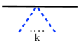
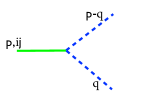
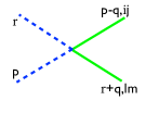
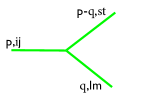
Figure 1: The vertices which contribute to the calculation of the static two-body potential up to fifth PN order are shown. The first diagram shows the matter-$\phi^{k}$ vertex, where the solid black lines stand for the non-dynamical external sources. In the three bulk vertices the solid green lines correspond to tensor fields, whereas the blue dashed lines correspond to scalar fields. The external momenta are $p$, $q$, $r$ and the indices of the tensor fields are given by $i$, $j$, $l$, $m$, $s$, $t$.

In fig. 1 the four vertices which are required for the calculation of the static contribution to the two-body potential up to 5th PN order are shown. From the point-particle action one obtains the first vertex of fig. 1, while the remaining three originate from the bulk action. The bulk vertices are distinguished by the fact that they contain either zero or two scalar fields. A typical Feynman diagram is then for example given by the tree-level graph which is shown in fig. 2. Its calculation delivers the well known Newton potential.

Figure 2: The 0PN diagram is shown.

3 Calculational strategy and factorization property

For the calculation of the static part of the two-body potential up to fifth PN order we consider only the classic contribution of our Feynman diagrams and do not take into account any quantum corrections. In general the original gravity Feynman diagrams depend on the ingoing and outgoing momenta $p_{1}$, $p_{2}$, $p_{3}$ and $p_{4}$, like shown in fig. 3, however, it turns out that the corresponding loop integrals are only functions of the momentum transfer $p_{3}-p_{2}=p=p_{1}-p_{4}$. As a result of this the corresponding loop integrals can be represented by self-energy type diagrams as illustrated in fig. 3, see also ref. [21].

=    

Figure 3: An illustration of the mapping of gravity Feynman diagrams to self-energies as used in ref. [21].

The contribution of a given amplitude to the two-body potential $V$ is obtained by performing the Fourier transform, i.e. going from momentum to coordinate space:

$$V={\rm{i}}\lim_{d\to 3}\int_{p}e^{{\rm{i}}p\cdot r}\;\;\raisebox{-22.76228pt}{\includegraphics[width=34.14322pt]{QFT_bubble}}\;\;\;\sim\;\;\;\raisebox{-14.22636pt}{\includegraphics[width=36.98866pt]{QFT_bubble_closed}}\;\longrightarrow\;\raisebox{-11.38092pt}{\includegraphics[width=34.14322pt]{QFT_bubble_shrunk}}\;.$$ (5)

In ref. [38] a theorem was shown, which states that

static graphs at odd $(2n+1)$-PN orders are factorizable,

with $n\in\mathbb{N}_{0}$. A factorizable graph has at least one matter-$\phi^{k}$ vertex with $k>1$ (see. fig. 1), while a prime graph contains only matter-$\phi^{k}$ vertices with $k=1$ [38]. The factorization property allows one to recursively determine a given odd PN order from the known lower PN ones. This strongly simplifies the determination of odd higher PN orders compared to performing a direct calculation of the appearing loop integrals, which becomes increasingly difficult with an increasing number of loops. The factorization becomes apparent diagrammatically when doing the Fourier transform of the amplitude to coordinate space as shown in eq. (5). The additional integration over $p$ can be interpreted as an additional loop integration, which can be visualized by joining the external legs of the self-energy into an additional propagator-like line and pinching it to a point [38] as it is illustrated on the r.h.s. of eq. (5).

The contribution of a factorizable graph to the potential can then just be obtained by multiplying together the results for the lower PN subgraphs [38]

$$V_{n}^{\rm{\tiny{factorizable}}}=\left(V_{L,n_{1}}\times V_{R,n_{2}}\right)\times{\mathcal{K}}\times{\mathcal{C}},$$ (6)

with $n=n_{1}+n_{2}+1$, where $V_{L,n_{1}}$ and $V_{R,n_{2}}$ is the potential of the left and right subgraph. The factor $\mathcal{K}$ takes into account the new matter-$\phi^{k}$ vertex which emerges through glueing the two subgraphs together. The factor $\mathcal{C}$ is a combinatoric factor.

In order to illustrate this method let us consider the well known static odd 1PN and 3PN orders. The 1PN potential can be obtained from a single static diagram. According to the factorization theorem, it can be decomposed in terms of two Newton diagrams

$$\hskip 19.91684pt\begin{minipage}{56.9055pt} \begin{center} \includegraphics[width=71.13188pt]{1PNstatic.pdf} \end{center} \end{minipage}=\left(\begin{minipage}{42.67912pt} \begin{center} \includegraphics[width=36.98866pt]{Newton.pdf} \end{center} \end{minipage}\right)^{2}\times\frac{\begin{minipage}{34.14322pt} \includegraphics[width=36.98866pt]{particle2.pdf} \end{minipage}}{\left(\begin{minipage}{31.2982pt} \includegraphics[width=36.98866pt]{particle1.pdf}\end{minipage}\right)^{2}}\,,$$ (7)

where the individual factors on the $r.h.s.$ indeed lead to the known result for the one-loop diagram,

$$\;\;\;\qquad\frac{G_{N}^{2}m_{1}^{2}m_{2}}{2r^{2}}=\left(\!\!-\frac{G_{N}m_{1}m_{2}}{r}\right)^{2}\!\times{{G_{N}m_{2}/2}\over\left(\sqrt{G_{N}}m_{2}\!\right)^{2}}\,.$$ (8)

In this example, the factor ${\cal K}$ of eq. (6) is given by the fraction on the $r.h.s.$ of eq. (7), while ${\cal C}=1$. We have adopted the convention that $m_{1(2)}$ refers to the bottom (top) line in the diagrams. The static 1PN potential is then given by ${V}^{({\rm 1PN})}_{\rm static}=\frac{G_{N}^{2}m_{1}^{2}m_{2}}{2r^{2}}+(m_{1}\leftrightarrow m_{2})$.

$\mbox{\footnotesize{A}}_{\mbox{\tiny{3PN}}}$

$\mbox{\footnotesize{B}}_{\mbox{\tiny{3PN}}}$

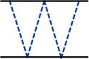
$\mbox{\footnotesize{C}}_{\mbox{\tiny{3PN}}}$

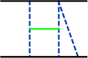
$\mbox{\footnotesize{D}}_{\mbox{\tiny{3PN}}}$

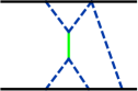
$\mbox{\footnotesize{E}}_{\mbox{\tiny{3PN}}}$

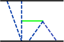
$\mbox{\footnotesize{F}}_{\mbox{\tiny{3PN}}}$

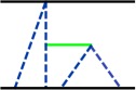
$\mbox{\footnotesize{G}}_{\mbox{\tiny{3PN}}}$

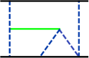
$\mbox{\footnotesize{H}}_{\mbox{\tiny{3PN}}}$

Figure 4: The 3PN graphs are shown. The first graph in the second line (bottom-left) does not contribute to the 3PN potential, because its 2PN subdiagram vanishes.

At the 3PN order there are eight static graphs which are shown in fig. 4. Their contributions to the Lagrangian were computed in [34]. In light of the factorization theorem, we identify two classes of diagrams:

1. In this set, we consider three diagrams composed out of four Newtonian factors, corresponding to the first three diagrams of fig. 4 ($\mbox{A}_{\mbox{\footnotesize{3PN}}}$, $\mbox{B}_{\mbox{\footnotesize{3PN}}}$, $\mbox{C}_{\mbox{\footnotesize{3PN}}}$). We represent them as:

$$\left(\begin{minipage}{48.36958pt} \hskip 2.84544pt \includegraphics[width=36.98866pt]{Newton.pdf} \end{minipage}\right)^{4}\,.$$ (9)

Their contribution to the 3PN potential is:

$${V}_{N^{4}} = \frac{1}{24}\frac{G_{N}^{4}m_{1}^{4}m_{2}}{r^{4}}+\frac{G_{N}^{4}m_{1}^{3}m_{2}^{2}}{r^{4}}+(m_{1}\leftrightarrow m_{2})\ .\qquad$$ (10)

2. The other five diagrams of fig. 4 ($\mbox{D}_{\mbox{\footnotesize{3PN}}}$, $\mbox{E}_{\mbox{\footnotesize{3PN}}}$, $\mbox{F}_{\mbox{\footnotesize{3PN}}}$, $\mbox{G}_{\mbox{\footnotesize{3PN}}}$, $\mbox{H}_{\mbox{\footnotesize{3PN}}}$), are built as products of one Newtonian term and the three static 2PN prime graphs, combined in all possible ways, schematically represented as:

$$\begin{minipage}{34.14322pt} \begin{center} \includegraphics[width=36.98866pt]{Newton.pdf} \end{center} \end{minipage}\!\!\!\times\left(\begin{minipage}{102.43008pt} \begin{center} \includegraphics[width=96.73918pt]{2PNstaticprime.pdf} \end{center} \end{minipage}\right)\ .$$ (11)

For illustration purposes, the factorization theorem can be verified for one of them:

$$\qquad\begin{minipage}{76.82234pt} \begin{center} \includegraphics[width=76.82234pt]{3PNexample.pdf} \end{center} \end{minipage}=\hskip 4.30554pt2\times\hskip 4.30554pt\begin{minipage}{42.67912pt} \begin{center} \includegraphics[width=36.98866pt]{Newton.pdf} \end{center} \end{minipage}\hskip 4.30554pt\times\begin{minipage}{69.70915pt} \begin{center} \includegraphics[width=69.70915pt]{2PNexample.pdf} \end{center} \end{minipage}\!\!\!\times\;\;\frac{\begin{minipage}{34.14322pt} \begin{center} \includegraphics[width=36.98866pt]{particle2.pdf} \end{center} \end{minipage}}{\left(\begin{minipage}{31.2982pt} \begin{center} \includegraphics[width=36.98866pt]{particle1.pdf} \end{center} \end{minipage}\right)^{2}}\,,\qquad\quad$$ (12)

(${\cal C}=2$ here) amounting to

$$\quad\qquad\frac{G_{N}^{4}m_{1}^{4}m_{2}}{3r^{4}}\;\;=\;\;2\times\left(\!-\frac{G_{N}m_{1}m_{2}}{r}\right)\times\left(\!-\frac{G^{3}_{N}m_{1}^{3}m_{2}}{3r^{3}}\right)\times{{G_{N}m_{2}/2}\over\left(\sqrt{G_{N}}m_{2}\right)^{2}}\,,\qquad$$ (13)

in agreement with [34]. The contribution to the potential from the five diagrams in class 2 is:

$${V}_{N\times{\rm 2PN}} = \frac{1}{3}\frac{G_{N}^{4}m_{1}^{4}m_{2}}{r^{4}}+5\frac{G_{N}^{4}m_{1}^{3}m_{2}^{2}}{r^{4}}+(m_{1}\leftrightarrow m_{2})\,.\qquad$$ (14)

The total static 3PN contribution of the diagrams belonging to classes 1 and 2 is, in agreement with the literature:

$${V}^{({\rm 3PN})}_{\rm static}={V}_{N^{4}}+{V}_{N\times{\rm 2PN}}=\frac{3}{8}\frac{G_{N}^{4}m_{1}^{4}m_{2}}{r^{4}}+6\frac{G_{N}^{4}m_{1}^{3}m_{2}^{2}}{r^{4}}+(m_{1}\leftrightarrow m_{2})\,.$$ (15)

4 The results

The static contribution to the two-body potential at fifths PN order can be determined recursively from the lower PN results with the help of the factorization property of ref. [38] as discussed in sec. 3. The 154 five-loop diagrams can be subdivided here into four classes according to their factorization property. The first class consist out of products of six Newtonian diagrams. The second class consists out of products of three Newtonian graphs and the prime 2PN diagrams. The third class are products of a Newtonian diagram and the 4PN prime graphs. Finally the last class are products of the 2PN prime graphs.

The ingredients which are needed in order to determine the static 5PN contribution are only the static 2PN and 4PN prime graphs. All static 5PN contributions can then be obtained through the factorization property. The static 2PN and 4PN prime graphs are known since long from literature, as discussed in sec. 1. In particular the static 4PN contribution has been computed in the EFT approach in ref. [21] by employing techniques for calculating Feynman diagrams which are used in high energy particle physics. The appearing 50 diagrams are subdivided into two sets. The first set contains simpler integrals which can be computed with the kite rule [39, 40]. The second set of four-loop integrals has been reduced systematically to a small set of seven master integrals (MI) with integration-by-parts identities [39, 40] using Laporta’s algorithm [41, 42]. They are shown in fig. 5.

$\mathcal{M}_{0,1}$

$\mathcal{M}_{1,1}$

$\mathcal{M}_{1,2}$

$\mathcal{M}_{1,3}$

$\mathcal{M}_{1,4}$

$\mathcal{M}_{2,2}$

$\mathcal{M}_{3,6}$

Figure 5: The master integrals appearing in the calculation of the static 4PN contribution are shown.

The reduction has been performed in two ways, with an in-house code based on Form [43, 44, 45] and with the program Reduze [46, 47]. Five of the seven MIs $\{\mathcal{M}_{0,1},\mathcal{M}_{1,1},\mathcal{M}_{1,2},\mathcal{M}_{1,3},\mathcal{M}_{1,4}\}$ can be calculated straightforwardly in a closed analytical form in $d$ dimensions. They are expressible in terms of $\Gamma$-functions. The MI $\mathcal{M}_{2,2}$ always appears multiplied by sufficient high positive powers of $\varepsilon=(d-3)$ in the amplitude, so that it drops out in the limit $\varepsilon\to 0$. The remaining seventh MI $\mathcal{M}_{3,6}$ is known in an expansion in $\varepsilon$ in refs. [48, 21, 49].

Having all even PN orders at hand, the static 5PN contribution to the gravitational two-body potential has been obtained for the first time in ref. [38] with the help of the factorization property. It reads:

$${V}^{({\rm 5PN})}_{\rm static}={5\over 16}{G_{N}^{6}m_{1}^{6}m_{2}\over r^{6}}+{91\over 6}{G_{N}^{6}m_{1}^{5}m_{2}^{2}\over r^{6}}+{653\over 6}{G_{N}^{6}m_{1}^{4}m_{2}^{3}\over r^{6}}+(m_{1}\leftrightarrow m_{2}).$$ (16)

The result has been checked in the test-particle limit, in which one considers the body with mass $m_{2}$ as a test particle in the gravitational field of the body with mass $m_{1}$, corresponding to the Schwarzschild limit which recovers the term linear in $m_{2}$ and with the highest power in $m_{1}$. At fifth PN order this check has been used for the first-time in ref. [38]. In this limit the static effective Lagrangian reads $\mathcal{L}^{m_{1}\gg m_{2}}_{\rm static}=-m_{2}\sqrt{1-G_{N}m_{1}/r}/\sqrt{1+G_{N}m_{1}/r}$. Its expansion permits to extract this contribution to the potential at each PN order. Hence, the Schwarzschild metric allows to predict the coefficients of the terms of the form ${G_{N}^{\ell}m_{1}^{\ell}m_{2}/r^{\ell}}$ at any $n$-th PN order with $\ell=n+1$, for example, at 6th PN order the coefficient of the term ${G_{N}^{7}m_{1}^{7}m_{2}/r^{7}}$ reads $-5/16$. Finally eq. (16) has been confirmed in ref. [50] by an independent calculation.

5 Summary and conclusion

We studied the gravitational two-body potential at fourth and fifth PN order in the EFT approach to GR in the static limit. Its calculation can be mapped onto the determination of four- and five-loop self-energies, which can be solved with tools commonly used in high-energy particle physics. We established a factorization property of the static diagrams appearing at odd PN orders, so that these contributions can be determined recursively from the lower PN order results and no loop integrals need to be computed. We verified the validity of our factorization theorem at the lower odd PN orders and applied it to the fifth PN order in order to do a first-time calculation of the static contributions to the gravitational two-body potential. The factorization property is also applicable to a large subset of even-PN diagrams, which simplifies their calculation. As a result of this the factorization property is a powerful tool to simplify higher order PN calculations.

- [1] A. Einstein, L. Infeld and B. Hoffmann, The Gravitational equations and the problem of motion, Annals Math. 39 (1938) 65–100.
- [2] Virgo, LIGO Scientific collaboration, B. P. Abbott et al., Observation of Gravitational Waves from a Binary Black Hole Merger, Phys. Rev. Lett. 116 (2016) 061102, [1602.03837].
- [3] LIGO Scientific collaboration, J. Aasi et al., Advanced LIGO, Class. Quant. Grav. 32 (2015) 074001, [1411.4547].
- [4] VIRGO collaboration, F. Acernese et al., Advanced Virgo: a second-generation interferometric gravitational wave detector, Class. Quant. Grav. 32 (2015) 024001, [1408.3978].
- [5] A. Taracchini, Y. Pan, A. Buonanno, E. Barausse, M. Boyle, T. Chu et al., Prototype effective-one-body model for nonprecessing spinning inspiral-merger-ringdown waveforms, Phys. Rev. D86 (2012) 024011, [1202.0790].
- [6] P. Schmidt, F. Ohme and M. Hannam, Towards models of gravitational waveforms from generic binaries II: Modelling precession effects with a single effective precession parameter, Phys. Rev. D91 (2015) 024043, [1408.1810].
- [7] T. Damour, Gravitational Radiation and the motion of compact bodies, in Les Houches Summer School on Gravitational Radiation Les Houches, France, June 2-21, 1982, 1982.
- [8] T. Damour and G. Schäfer, Lagrangians forn point masses at the second post-Newtonian approximation of general relativity, Gen. Rel. Grav. 17 (1985) 879–905.
- [9] T. Damour, P. Jaranowski and G. Schäfer, Dimensional regularization of the gravitational interaction of point masses, Phys. Lett. B513 (2001) 147–155, [gr-qc/0105038].
- [10] L. Blanchet, T. Damour and G. Esposito-Farese, Dimensional regularization of the third post-Newtonian dynamics of point particles in harmonic coordinates, Phys. Rev. D69 (2004) 124007, [gr-qc/0311052].
- [11] Y. Itoh and T. Futamase, New derivation of a third post-Newtonian equation of motion for relativistic compact binaries without ambiguity, Phys. Rev. D68 (2003) 121501, [gr-qc/0310028].
- [12] T. Damour, P. Jaranowski and G. Schäfer, Nonlocal-in-time action for the fourth post-Newtonian conservative dynamics of two-body systems, Phys. Rev. D89 (2014) 064058, [1401.4548].
- [13] T. Damour, P. Jaranowski and G. Schäfer, Fourth post-Newtonian effective one-body dynamics, Phys. Rev. D91 (2015) 084024, [1502.07245].
- [14] T. Damour, P. Jaranowski and G. Schäfer, Conservative dynamics of two-body systems at the fourth post-Newtonian approximation of general relativity, Phys. Rev. D93 (2016) 084014, [1601.01283].
- [15] L. Bernard, L. Blanchet, A. Bohé, G. Faye and S. Marsat, Fokker action of nonspinning compact binaries at the fourth post-Newtonian approximation, Phys. Rev. D93 (2016) 084037, [1512.02876].
- [16] L. Bernard, L. Blanchet, A. Bohé, G. Faye and S. Marsat, Energy and periastron advance of compact binaries on circular orbits at the fourth post-Newtonian order, Phys. Rev. D95 (2017) 044026, [1610.07934].
- [17] L. Bernard, L. Blanchet, A. Bohé, G. Faye and S. Marsat, Dimensional regularization of the IR divergences in the Fokker action of point-particle binaries at the fourth post-Newtonian order, Phys. Rev. D96 (2017) 104043, [1706.08480].
- [18] T. Marchand, L. Bernard, L. Blanchet and G. Faye, Ambiguity-Free Completion of the Equations of Motion of Compact Binary Systems at the Fourth Post-Newtonian Order, Phys. Rev. D97 (2018) 044023, [1707.09289].
- [19] L. Bernard, L. Blanchet, G. Faye and T. Marchand, Center-of-Mass Equations of Motion and Conserved Integrals of Compact Binary Systems at the Fourth Post-Newtonian Order, Phys. Rev. D97 (2018) 044037, [1711.00283].
- [20] S. Foffa and R. Sturani, Dynamics of the gravitational two-body problem at fourth post-Newtonian order and at quadratic order in the Newton constant, Phys. Rev. D87 (2013) 064011, [1206.7087].
- [21] S. Foffa, P. Mastrolia, R. Sturani and C. Sturm, Effective field theory approach to the gravitational two-body dynamics, at fourth post-Newtonian order and quintic in the Newton constant, Phys. Rev. D95 (2017) 104009, [1612.00482].
- [22] S. Foffa and R. Sturani, Conservative dynamics of binary systems to fourth Post-Newtonian order in the EFT approach I: Regularized Lagrangian, Phys. Rev. D100 (2019) 024047, [1903.05113].
- [23] S. Foffa, R. A. Porto, I. Rothstein and R. Sturani, Conservative dynamics of binary systems to fourth Post-Newtonian order in the EFT approach II: Renormalized Lagrangian, Phys. Rev. D100 (2019) 024048, [1903.05118].
- [24] M. Punturo et al., The Einstein Telescope: A third-generation gravitational wave observatory, Class. Quant. Grav. 27 (2010) 194002.
- [25] LISA collaboration, H. Audley et al., Laser Interferometer Space Antenna, 1702.00786.
- [26] L. Lindblom, B. J. Owen and D. A. Brown, Model Waveform Accuracy Standards for Gravitational Wave Data Analysis, Phys. Rev. D78 (2008) 124020, [0809.3844].
- [27] A. Antonelli, A. Buonanno, J. Steinhoff, M. van de Meent and J. Vines, Energetics of two-body Hamiltonians in post-Minkowskian gravity, Phys. Rev. D99 (2019) 104004, [1901.07102].
- [28] W. D. Goldberger and I. Z. Rothstein, An Effective field theory of gravity for extended objects, Phys. Rev. D73 (2006) 104029, [hep-th/0409156].
- [29] W. D. Goldberger, Les Houches lectures on effective field theories and gravitational radiation, in Les Houches Summer School - Session 86: Particle Physics and Cosmology: The Fabric of Spacetime Les Houches, France, July 31-August 25, 2006, 2007, hep-ph/0701129.
- [30] S. Foffa and R. Sturani, Effective field theory methods to model compact binaries, Class. Quant. Grav. 31 (2014) 043001, [1309.3474].
- [31] I. Z. Rothstein, Progress in effective field theory approach to the binary inspiral problem, Gen. Rel. Grav. 46 (2014) 1726.
- [32] R. A. Porto, The effective field theorist’s approach to gravitational dynamics, Phys. Rept. 633 (2016) 1–104, [1601.04914].
- [33] M. Levi, Effective Field Theories of Post-Newtonian Gravity: A comprehensive review, 1807.01699.
- [34] S. Foffa and R. Sturani, Effective field theory calculation of conservative binary dynamics at third post-Newtonian order, Phys. Rev. D84 (2011) 044031, [1104.1122].
- [35] L. Blanchet, Gravitational radiation from post-Newtonian sources and inspiralling compact binaries, Living Reviews in Relativity 5 (2002) .
- [36] B. Kol and M. Smolkin, Non-Relativistic Gravitation: From Newton to Einstein and Back, Class. Quant. Grav. 25 (2008) 145011, [0712.4116].
- [37] B. Kol and M. Smolkin, Classical Effective Field Theory and Caged Black Holes, Phys. Rev. D77 (2008) 064033, [0712.2822].
- [38] S. Foffa, P. Mastrolia, R. Sturani, C. Sturm and W. J. Torres Bobadilla, Static two-body potential at fifth post-Newtonian order, Phys. Rev. Lett. 122 (2019) 241605, [1902.10571].
- [39] F. V. Tkachov, A Theorem on Analytical Calculability of Four Loop Renormalization Group Functions, Phys. Lett. B100 (1981) 65–68.
- [40] K. G. Chetyrkin and F. V. Tkachov, Integration by Parts: The Algorithm to Calculate beta Functions in 4 Loops, Nucl. Phys. B192 (1981) 159–204.
- [41] S. Laporta and E. Remiddi, The Analytical value of the electron (g-2) at order in QED, Phys. Lett. B379 (1996) 283–291, [hep-ph/9602417].
- [42] S. Laporta, High precision calculation of multiloop Feynman integrals by difference equations, Int. J. Mod. Phys. A15 (2000) 5087–5159, [hep-ph/0102033].
- [43] J. A. M. Vermaseren, New features of FORM, math-ph/0010025.
- [44] J. A. M. Vermaseren, Tuning FORM with large calculations, Nucl. Phys. Proc. Suppl. 116 (2003) 343–347, [hep-ph/0211297].
- [45] M. Tentyukov and J. A. M. Vermaseren, Extension of the functionality of the symbolic program FORM by external software, Comput. Phys. Commun. 176 (2007) 385–405, [cs/0604052].
- [46] C. Studerus, Reduze-Feynman Integral Reduction in C++, Comput. Phys. Commun. 181 (2010) 1293–1300, [0912.2546].
- [47] A. von Manteuffel and C. Studerus, Reduze 2 - Distributed Feynman Integral Reduction, 1201.4330.
- [48] R. N. Lee and K. T. Mingulov, Introducing SummerTime: a package for high-precision computation of sums appearing in DRA method, Comput. Phys. Commun. 203 (2016) 255–267, [1507.04256].
- [49] T. Damour and P. Jaranowski, Four-loop static contribution to the gravitational interaction potential of two point masses, Phys. Rev. D95 (2017) 084005, [1701.02645].
- [50] J. Blümlein, A. Maier and P. Marquard, Five-Loop Static Contribution to the Gravitational Interaction Potential of Two Point Masses, Phys. Lett. B800 (2020) 135100, [1902.11180].