Adaptive Dynamic Model Averaging with an Application to House Price Forecasting

Abstract

Dynamic model averaging (DMA) combines the forecasts of a large number of dynamic linear models (DLMs) to predict the future value of a time series. The performance of DMA critically depends on the appropriate choice of two forgetting factors. The first of these controls the speed of adaptation of the coefficient vector of each DLM, while the second enables time variation in the model averaging stage. In this paper we develop a novel, adaptive dynamic model averaging (ADMA) methodology. The proposed methodology employs a stochastic optimisation algorithm that sequentially updates the forgetting factor of each DLM, and uses a state-of-the-art non-parametric model combination algorithm from the prediction with expert advice literature, which offers finite-time performance guarantees. An empirical application to quarterly UK house price data suggests that ADMA produces more accurate forecasts than the benchmark autoregressive model, as well as competing DMA specifications.

Keywords: Adaptive forgetting; Stochastic optimisation; Prediction with Expert Advice; Dynamic linear model; Housing market

1 Introduction

A growing empirical literature provides strong evidence in favour of structural instability in many macroeconomic relations (Stock and Watson, 1996; Koop and Potter, 2007; Ng and Wright, 2013). Structural instability is crucial because, if left unaccounted for, it can have detrimental consequences for statistical inference and forecasting (Clements and Hendry, 1998; Pesaran et al., 2006; Giacomini and Rossi, 2009; Rossi, 2013).

Dynamic Model Averaging (DMA) is an econometric methodology that can accommodate time variations in both model parameters and model specification (Raftery et al., 2010). This methodology has gained increasing popularity in recent years for predicting various economic variables, such as inflation (Koop and Korobilis, 2012; Catania and Nonejad, 2018), carbon prices (Koop and Tole, 2013), exchange rates (Byrne et al., 2018), equity returns (Dangl and Halling, 2012), and property price growth (Bork and Møller, 2015). DMA creates a Dynamic Linear Model (DLM) for every possible subset of predictors and combines the forecasts of these models using weights that adapt over time (Raftery et al., 2010). To adapt to changes in the data generating distribution, DMA involves two parameters, called forgetting factors. The first forgetting factor is part of the DLM formulation, while the second is involved in the model averaging phase. These parameters allow a continuous trade-off between estimation in a static environment, and re-initialising the estimation process by discarding all past information, which is appropriate after a structural break. It is therefore not surprising that the choice of forgetting factors is critical to the forecast performance of DMA.

Initial work by Raftery et al. (2010) and Koop and Korobilis (2012) considered both forgetting factors to be user-defined and constant. However, in general, the type of structural change in economic relationships is unknown and may vary considerably over time (Chen and Hong, 2012). Structural breaks due to changes in regulatory conditions, in the behaviour of consumers and firms or in the preferences of policy makers constitute prominent examples where periods during which the data generating process is static are interrupted by episodes of abrupt change (Pesaran et al., 2006; Kapetanios and Tzavalis, 2010). In this setting, and more generally whenever the speed or type of change in the data generating process is not constant, there does not exist a single choice of forgetting factors that is optimal for the entire length of a time series.

The DMA formulation of Dangl and Halling (2012), adopted by a number of more recent works (Catania and Nonejad, 2018; Byrne et al., 2018) involves no forgetting in the model averaging stage, and treats the choice of the DLM forgetting factor as an additional dimension of model uncertainty. In particular, the user specifies a grid of forgetting factor values, and the posterior distribution of this parameter is updated at every time step by marginalising over all DLM specifications. The Bayesian approach of Dangl and Halling (2012) effectively assumes that the appropriate choice of the DLM forgetting factor is constant over time, and identical across models. McCormick et al. (2012) propose a similar approach that involves a grid of values for both forgetting factors. They propose to use the forgetting factors that maximise the predictive likelihood for each DLM specification to avoid the computational cost of Bayesian updating.

In this paper, we develop an adaptive dynamic model averaging (ADMA) methodology that consists of two components. The first involves the use of stochastic optimisation to identify the forgetting factor that minimises the expected one-step-ahead squared forecast error of each DLM. This leads to a fully online and data-driven algorithm which we call Adaptive Forgetting DLM (AF-DLM). As we show in the experimental results section AF-DLM is effective under different types of change in the data generating process, including cases in which the speed or type of change is variable over time. AF-DLM is also computationally less expensive than previous approaches since it does not involve a grid of forgetting factor values.

The second component of ADMA deals with model averaging. We show that the speed with which DMA weights respond to more recent observations is determined not only by the choice of the corresponding forgetting factor, but also by the mechanism that prevents underflow (weights becoming equal to machine zero). Therefore any approach to control the adaptability of DMA weights by tuning only the second forgetting factor is inherently limited. We propose to replace the current model averaging approach with the ConfHedge model combination algorithm from the field of machine learning known as prediction with expert advice (V’yugin and Trunov, 2019). In addition to being parameter-free, ConfHedge is currently the only model combination algorithm whose one-step-ahead squared forecast error over a finite number of time steps is within a known bound of the one-step-ahead squared forecast error of the optimal sequence of forecasting models.

To assess the effectiveness of the proposed methodology, we provide an in-depth empirical evaluation of ADMA on the task of forecasting UK house prices. The motivation for this application is twofold. First, although the latest boom-bust episode in real estate markets and its decisive role in the Great Recession has generated a vast interest in the behavior of international housing markets, the academic literature on house price forecastability is relatively small (especially when compared to the literature on other assets such as stock prices and exchange rates), and mainly concentrates on the US market (see, e.g., Rapach and Strauss, 2009; Ghysels et al., 2013; Bork and Møller, 2015). In the UK, similarly to the US, housing activities account for a large fraction of GDP and of households’ expenditures, real estate property comprises the largest component of private wealth (excluding private pensions), and mortgage debt constitutes the main liability of households (Office for National Statistics, 2018). Thus, accurate forecasts of UK real estate prices are crucial for private investors and policy makers. Second, recent empirical evidence suggests that the relationship between real estate valuations and conditioning macro and financial variables displays time-varying patterns (Aizenman and Jinjarak, 2014; Anundsen, 2015; Paul, 2018). This makes housing markets an ideal setting for the application of dynamic econometric models.

In summary, the results of our empirical application suggest that ADMA offers significant forecasting gains relative to a linear autoregressive (AR) benchmark, as well as a battery of competing dynamic and static forecasting models. They also indicate that the best house predictors substantially differ over time and across regions. In-sample stability tests also support the conclusion that the data generating process of regional UK house prices is subject to structural instability.

The remaining paper is organised as follows. Section 2 presents the ADMA methodology. In Section 3 we assess the proposed AF-DLM on simulated time series exhibiting different types of dynamics. Section 4 is devoted to the comparative evaluation of ADMA against alternative forecasting models on the task of predicting UK regional house prices. The paper ends with concluding remarks in Section 5.

2 Methodology

This section is divided into three parts. The first part provides a brief outline of the DMA methodology. The second part deals with the development of the stochastic optimisation approach to sequentially adapt the forgetting factor in a single DLM. The last part discusses limitations of existing model combination methods and presents the ConfHedge algorithm.

2.1 Dynamic Model Averaging

For a set of $D$ covariates, DMA creates a DLM for each possible subset (excluding the empty set), giving rise to $K=2^{D}-1$ models, $M_{1},\ldots,M_{K}$. Model $M_{k}$ is defined by,

$$\theta^{(k)}_{t+1} =\theta^{(k)}_{t}+\omega^{(k)}_{t+1}, \omega^{(k)}_{t+1}\sim\mathcal{N}\left(0,W^{(k)}_{t+1}\right),$$ (1)

$$y_{t+1} =x_{t+1}^{(k)\top}\theta^{(k)}_{t+1}+\varepsilon^{(k)}_{t+1}, \varepsilon^{(k)}_{t+1}\sim\mathcal{N}\left(0,V^{(k)}_{t+1}\right),$$ (2)

where $\theta^{(k)}_{t}\in\mathbb{R}^{d}$ denotes the coefficient vector and $x^{(k)}_{t}\in\mathbb{R}^{d}$ is the covariate vector (including a constant) of $M_{k}$ at time $t$. Eq. (1), known as the state-transition equation, determines the dynamics of the unobserved coefficient vector. Eq. (2), called the observation or measurement equation, links the response, $y_{t+1}$, to the coefficients and the covariates. The errors, or noise terms, $\omega^{(k)}_{t+1}$ and $\varepsilon^{(k)}_{t+1}$ in Eqs. (1) and (2), respectively, are assumed to be independent normally distributed random variables. The state transition covariance matrix, $W^{(k)}_{t+1}$, and the observational variance, $V^{(k)}_{t+1}$, are typically unknown.

The DMA forecast, $\hat{y}_{t+1}$, is obtained through a convex combination of the forecasts of the $K$ DLMs,

$$\hat{y}_{t+1}=\sum_{k=1}^{K}p(M_{k}|\mathcal{F}^{(k)}_{t})\,\hat{y}^{(k)}_{t+1},$$ (3)

where $\hat{y}^{(k)}_{t+1}$ is the prediction by model $M_{k}$, and $p(M_{k}|\mathcal{F}^{(k)}_{t})$ is the probability (weight) assigned to $M_{k}$ conditional on the information available at time $t$, $\mathcal{F}^{(k)}_{t}$. The information set is defined as, $\mathcal{F}^{(k)}_{t}=\{y_{t},\ldots,y_{1},x^{(k)}_{t+1},x^{(k)}_{t},\ldots,x^{(k)}_{1},\mathrm{Priors}_{t=0}\}$, and contains the choice of priors, the realisations of the covariate vector and of the response up to time $t$, as well as the covariate vector at time $t+1$, $x^{(k)}_{t+1}$, required to predict $y_{t+1}$.

2.2 Dynamic Linear Model with Forgetting

Because we consider a single DLM with forgetting throughout this subsection, we drop the superscript $(k)$ to simplify notation. We adopt the DLM formulation proposed of Dangl and Halling (2012), in which the prior distribution for the coefficients vector, $\theta_{0}$, is Gaussian; the measurement variance, $V_{t}=V$, is constant over time; and an inverse-gamma distributed prior for $V$ is used. Consequently,

$$V|\mathcal{F}_{0} \sim\mathrm{IG}\left(\frac{1}{2},\frac{1}{2}S_{0}\right),$$ (4)

$$\theta_{0}|\mathcal{F}_{0},V \sim\mathcal{N}\left(0,gI\right),$$ (5)

which enables a conjugate Bayesian analysis. The model specification and the assumptions about the priors imply that,

$$V|\mathcal{F}_{t} \sim\mathrm{IG}\left(\frac{n_{t}}{2},\frac{n_{t}}{2}S_{t}\right),$$ (6)

where $S_{t}$ is the mean of the estimate of $V$ at time $t$, and $n_{t}$ stands for the associated degrees of freedom. Conditional on $V$ the posterior distribution of the coefficient vector is Gaussian,

$$\theta_{t}|\mathcal{F}_{t},V \sim\mathcal{N}\left(\hat{\theta}_{t},\frac{V}{S_{t}}C_{t}\right),$$ (7)

where $\hat{\theta}_{t}$ is the point estimate of $\theta_{t}$, and $C_{t}$ is the estimator for the conditional covariance matrix for $\theta_{t}$. Integrating out $V$, the posterior becomes a multivariate $t$-distribution,

$$\theta_{t}|\mathcal{F}_{t} \sim\mathcal{T}_{n_{t}}\left(\hat{\theta}_{t},C_{t}\right).$$ (8)

The prior distribution for the coefficient vector at the next time-step is,

$$\theta_{t+1}|\mathcal{F}_{t}\sim\mathcal{T}_{n_{t}}\left(\hat{\theta}_{t},C_{t}+W_{t+1}\right).$$ (9)

For a generic DLM, $W_{t+1}$ can be sequentially estimated, but the associated computational cost is prohibitive for a method like DMA which uses $2^{D}-1$ DLMs. The distinctive feature of the approach of Raftery et al. (2010) is that it avoids altogether the estimation of $W_{t+1}$ by setting,

$$W_{t+1}=\frac{1-\lambda}{\lambda}C_{t},$$ (10)

where $\lambda\in(0,1]$ is the forgetting factor parameter. This simplifies Eq. (9) to,

$$\theta_{t+1}|\mathcal{F}_{t}\sim\mathcal{T}_{n_{t}}\left(\hat{\theta}_{t},\lambda^{-1}C_{t}\right).$$ (11)

The forgetting factor in Eq. (10) allows a continuous range between estimation in a static environment and completely discarding all past data which is appropriate in response to a structural break. Specifically, setting $\lambda=1$ corresponds to $W_{t}=\mathbf{0}$ and thus reduces the DLM to a static linear model. On the other hand, as $\lambda$ tends to zero $W_{t}$ tends to infinity. This inflates the uncertainty about $\theta_{t+1}$ (see Eq. (11)), which effectively re-initialises the estimation process. Intermediate values of $\lambda$ correspond to a random walk process for $\theta$ in which periods of high estimation error in the coefficients coincide with periods of high variability, and vice versa.

The prior distribution (predictive density) of $y_{t+1}$ conditional on $\mathcal{F}_{t}$ is,

$$y_{t+1}|\mathcal{F}_{t} \sim\mathcal{T}_{n_{t}}\left(x_{t+1}^{\top}\hat{\theta}_{t},\;Q_{t+1}\right),$$ (12)

$$Q_{t+1} =\lambda^{-1}x_{t+1}^{\top}C_{t}x_{t+1}+S_{t}.$$ (13)

Once the actual value $y_{t+1}$ is observed, we can compute the forecast error,

$$\hat{\varepsilon}_{t+1}=y_{t+1}-x_{t+1}^{\top}\hat{\theta}_{t},$$ (14)

and update the prior distributions of the coefficient vector and the measurement variance through Eqs (15)–(18). The degrees of freedom and the estimator of the observational variance are updated according to,

$$n_{t+1} =n_{t}+1,$$ (15)

$$S_{t+1} =S_{t}+\frac{S_{t}}{n_{t+1}}\left(\frac{\hat{\varepsilon}^{2}_{t+1}}{Q_{t+1}}-1\right).$$ (16)

The point estimate and the estimator of the covariance matrix of $\theta_{t+1}$ are obtained by,

$$\hat{\theta}_{t+1} =\hat{\theta}_{t}+A_{t+1}\hat{\varepsilon}_{t+1},$$ (17)

$$C_{t+1} =\lambda^{-1}C_{t}+A_{t+1}A_{t+1}^{\top}Q_{t+1},$$ (18)

where

$$A_{t+1}=\frac{\lambda^{-1}C_{t}x_{t+1}}{Q_{t+1}},$$ (19)

is a coefficient vector (known as the Kalman gain), which measures the information content of $y_{t+1}$ in relation to the precision of the estimated regression coefficient.

Adaptive Forgetting

We are now in a position to describe the adaptive forgetting DLM (AF-DLM). The approach we propose is motivated by the adaptive recursive least squares algorithm (Haykin, 2002). The central idea underlying this approach is that the optimal forgetting factor minimises the expectation of the one-step-ahead squared forecast error,

$$\lambda^{\star}_{t}=\operatorname*{arg\,min}_{\lambda\in(0,1]}\mathbb{E}\left[\frac{1}{2}\left(y_{t+1}-x_{t+1}^{\top}\hat{\theta}_{t}\right)^{2}\right].$$ (20)

Since the expectation in the above equation is not available in analytical form it is not feasible to directly optimise it. However, the one-step-ahead squared forecast error,

$$J_{t+1}=\frac{1}{2}\left(y_{t+1}-x_{t+1}^{\top}\hat{\theta}_{t}\right)^{2},$$ (21)

is an unbiased estimator of the expectation in Eq. (20). Stochastic optimisation algorithms are designed to optimise the expected value of a function which depends on a set of random variables. The most widely used stochastic optimisation algorithms involve first-order information and are hence variations of stochastic gradient descent. The term stochastic gradient in this context refers to the fact that the gradient of $J_{t+1}$ (which is an unbiased estimate of the gradient of $\mathbb{E}_{X,Y}[J_{t+1}]$) is used.

To use stochastic gradient descent to minimise the expected one-step-ahead squared forecast error we need an expression for the derivative of $J_{t+1}$ with respect to $\lambda$. Applying the chain rule produces,

$$\frac{\partial J_{t+1}}{\partial\lambda} =\frac{\partial J_{t+1}}{\partial\hat{\theta}_{t}}\,\frac{\partial\hat{\theta}_{t}}{\partial\lambda},$$

$$=-\hat{\varepsilon}_{t+1}x_{t+1}^{\top}\,\frac{\partial\hat{\theta}_{t}}{\partial\lambda}.$$ (22)

To obtain $\frac{\partial\hat{\theta}_{t}}{\partial\lambda}$ we differentiate the update equation for $\hat{\theta}_{t}$, Eq. (17), with respect to $\lambda$. Such an approach is utilised in a number of adaptive linear filters (Haykin, 2002), in online neural network training (Almeida et al., 1999; Schraudolph, 1999; Baydin et al., 2018), as well as in streaming data classifiers (Pavlidis et al., 2011; Anagnostopoulos et al., 2012). The outcome of this differentiation is,

$$\frac{\partial\hat{\theta}_{t}}{\partial\lambda} =\nabla_{\lambda}\left\{\hat{\theta}_{t-1}+A_{t}\hat{\varepsilon}_{t}\right\}$$

$$=(I-A_{t-1}x_{t}^{\top})\frac{\partial\hat{\theta}_{t-1}}{\partial\lambda}+\frac{\hat{\varepsilon}_{t}}{S_{t-1}}\left(\frac{\partial C_{t}}{\partial\lambda}x_{t}-A_{t-1}\frac{\partial S_{t-1}}{\partial\lambda}\right).$$ (23)

The derivation of all the necessary quantities to estimate $\frac{\partial\hat{\theta}_{t}}{\partial\lambda}$ is lengthy and is hence provided in Appendix A.

Using the gradient $\frac{\partial J_{t+1}}{\partial\lambda}$, AF-DLM updates the value of $\lambda$ at each time-step through the highly influential adaptive moment estimation (ADAM) stochastic gradient descent algorithm (Kingma and Ba, 2015). ADAM uses adaptive estimates of the first two moments of the stochastic gradient to tune the crucial step-size parameter of the gradient descent algorithm. ADAM has been shown to be effective in a wide range of challenging optimisation problems; it is straightforward to implement; and is capable of handling non-stationary objective functions (Baydin et al., 2018). The latter aspect is particularly important for our purposes since the optimal value of $\lambda$ is itself time-varying for time series that exhibit structural breaks, or more generally non-constant dynamics.

2.3 Model Averaging

In this section we discuss the model averaging component of DMA. Recall that according to Eq. (3) the DMA forecast, $\hat{y}_{t+1}$, is a convex combination of the forecasts produced by the $K$ DLMs. Let $p(M_{k}|\mathcal{F}_{t})$ denote the probability (weight) of model $M_{k}$ conditional on the information set $\mathcal{F}_{t}$. The following definition of $p(M_{k}|\mathcal{F}_{t})$ accommodates all DMA variants,

$$p(M_{k}|\mathcal{F}_{t}) =\frac{p(y_{t}|M_{k},\mathcal{F}_{t-1})\left[p(M_{k}|\mathcal{F}_{t-1})^{\alpha}+c\right]}{\sum_{m=1}^{K}p(y_{t}|M_{m},\mathcal{F}_{t-1})\left[p(M_{m}|\mathcal{F}_{t-1})^{\alpha}+c\right]}.$$ (24)

Ignoring the constant $c$ and expanding Eq. (24) gives,

$$p(M_{k}|\mathcal{F}_{t}) =\frac{p(M_{k}|\mathcal{F}_{0})^{\alpha^{t}}\prod_{j=1}^{t}p\left(y_{j}|M_{k},\mathcal{F}_{j-1}\right)^{\alpha^{t-j}}}{\sum_{m=1}^{K}p(M_{m}|\mathcal{F}_{0})^{\alpha^{t}}\prod_{j=1}^{t}p\left(y_{j}|M_{m},\mathcal{F}_{j-1}\right)^{\alpha^{t-j}}},$$

$$\propto\prod_{j=1}^{t}p(y_{j}|M_{k},\mathcal{F}_{j-1})^{\alpha^{t-i}},$$

where typically, $p(M_{k}|\mathcal{F}_{0})=1/K$. The last equation highlights that $\alpha$ controls the rate at which past information is discounted.

The recommendations in the literature are to set the forgetting factor $\alpha$ either equal to one (which corresponds to Bayesian Model Averaging), or very close to unity. In particular, Dangl and Halling (2012) and Byrne et al. (2018) use $\alpha=1$, while in the eDMA R package of Catania and Nonejad (2018) the default is $\alpha=0.99$. Raftery et al. (2010) and Koop and Korobilis (2012) recommend using $\lambda=\alpha$. Specifically, Raftery et al. (2010) recommend $\lambda=\alpha=0.99$, while Koop and Korobilis (2012) consider two values $\lambda,\alpha\in\{0.95,0.99\}$. Only Raftery et al. (2010) mention the small positive constant, $c$, in Eq. (24) which is included to avoid the weight of any model becoming equal to machine zero. Such a constant is present in the DMA implementation of Koop and Korobilis (2012), but not in the R package eDMA (Catania and Nonejad, 2018). The example we discuss next aims to illustrate that the speed with which model probabilities adapt in response to changes in the optimal model specification depends critically on $c$.

For simplicity we consider a problem involving only three models whose coefficients at every time-step are known. The observational variance of each model is also known and constant over time. The response at each time-step is generated from one of the three models, but the identity of this model is unknown. In this setting no generality is lost if we assume that for every model, $y_{t}^{(k)}|\theta_{t}^{(k)},x_{t}\sim\mathcal{N}(\mu_{k},V_{k})$, for all $t=1,\ldots,T$, and $k=1,2,3$. Thus we assume $y^{(1)}|\theta_{t}^{(1)},x_{t}\sim\mathcal{N}(1,4)$, $y^{(2)}|\theta_{t}^{(2)},x_{t}\sim\mathcal{N}(0,0.64)$, and $y^{(3)}|\theta_{t}^{(3)},x_{t}\sim\mathcal{N}(-2.5,0.09)$. We construct a time series of length $T=300$ by sampling $y_{t}$ from $M_{1}$ for $t=1,\ldots,100$, from $M_{2}$ for $t=101,\ldots,200$, and from $M_{3}$ for $t=201,\ldots,300$. The three models are assigned equal prior probabilities.

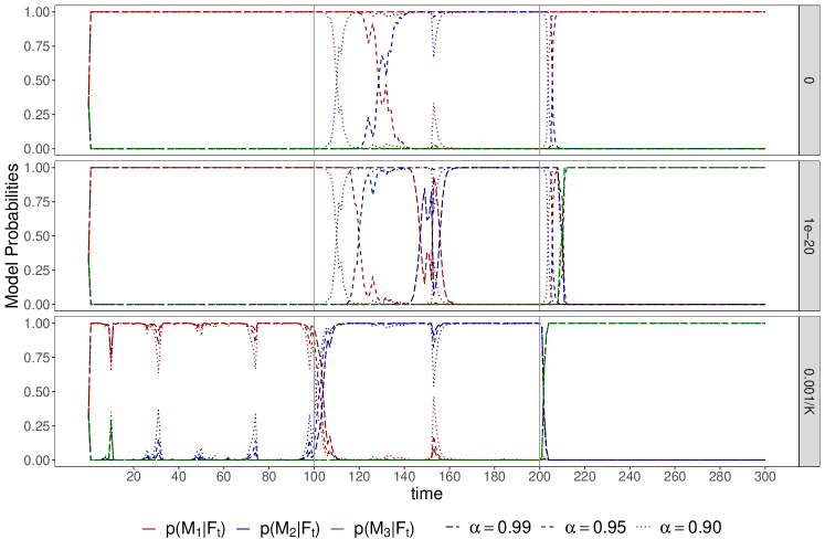
Figure 1: Probabilities determined through Eq. (24) for forgetting factor values, $\alpha\in\{0.99,0.95,0.9\}$, and values of  $c\in\{0,10^{-20},0.001/K\}$.

Figure 1 depicts the evolution of the weights of the three models using red, blue and green colour respectively. The three subfigures correspond to $c=0,10^{-20},10^{-3}/3$, as recommended by Catania and Nonejad (2018); Koop and Korobilis (2012) and Raftery et al. (2010), respectively. Within each subfigure a different type of dashed line is used to distinguish between the three values of the forgetting factor, $\alpha\in\{0.99,0.95,0.9\}$. Note that $\alpha=0.9$ is much lower than any recommendation in the literature, and is only included to explore the extent to which this forgetting factor enables adaptation. Finally, the two grey vertical lines depict the timing of the change points at $t=100,200$.

The top subfigure corresponds to $c=0$. For this setting using $\alpha=0.99$ causes the probability of $M_{1}$ to be effectively equal to one throughout the simulation despite the two change points. This occurs because the weights of models $M_{2}$ and $M_{3}$ are equal to machine zero by time-step $t=100$. A lower value of $\alpha$ allows the weights to adapt correctly to the first change point, but the response is slow even when $\alpha=0.9$. However, by time-step $t=200$ the weight assigned to $M_{3}$ is equal to zero for both $\alpha=0.95,0.9$. Therefore when $c=0$ not even very aggressive forgetting, $\alpha=0.9$, is sufficient for Eq. (24) to correctly identify the optimal model after the second change point. Instead $M_{1}$ is assigned a weight of one. Introducing a small constant, $c=10^{-20}$, (middle subfigure) enables the weights to adapt correctly in response to both change points for all values of $\alpha$. We see however that for $\alpha=0.99$ approximately 50 time-steps are required after the first change point for the weight assigned to $M_{1}$ to become noticeably lower than one. Although the response to the second change point is faster, notice that for $\alpha=0.95$ there is a short period immediately after the change point during which the weight of $M_{1}$ (rather than $M_{3}$) increases abruptly. The final subfigure corresponds to the case $c=10^{-3}/3$. A larger constant enables the weights to adapt much faster in response to both change points. Notice for instance that for $c=10^{-3}/3$ and $\alpha=0.99$ model probabilities adjust faster after the first change point, compared to the case when $\alpha=0.9$ but $c=10^{-20}$. However, a larger value of $c$ also induces much higher variability during periods in which the data generating process is static.

The above example demonstrates that the choice of $c$ in Eq. (24) is at least as important as that of $\alpha$. Therefore any approach focused only on tuning $\alpha$ is not sufficient to fully control the speed with which model probabilities in DMA adapt. We propose to use the ConfHedge algorithm from the field of machine learning known as prediction with expert advice (V’yugin and Trunov, 2019). As we discuss next ConfHedge has very appealing theoretical properties and is parameter-free.

Prediction with expert advice studies the following online learning problem (Cesa-Bianchi and Lugosi, 2006). At time-step, $t+1$, each of the $K$ forecasting models, called experts, provides a forecast, $\hat{y}^{(k)}_{t+1}$. An aggregating algorithm predicts $\hat{y}_{t+1}$ through a convex combination of the experts’ forecasts. After observing $y_{t+1}$, the weight of every expert is updated based on a measure of forecast error, called loss. In a static environment, the goal is to design weight updates that guarantee that the loss of the aggregating algorithm is never much larger than the cumulative loss of the best expert, or the best convex combination of the losses of the experts. In a dynamic environment the expert (or convex combination of experts) that achieve the lowest loss may differ across segments of the time series, and comparing against the best expert over the entire time series length can result in algorithms with poor forecast performance. To address this issue consider a partition of the time series into at most $L+1$ segments, $1<t_{(1)}<t_{(2)}<\cdots<t_{(L)}<T$, and allow the best expert (or convex combination of experts) to differ across elements of this partition. The best partition into at most $L+1$ segments is the one for which the optimal sequence of experts (or convex combination of experts) achieves the lowest cumulative loss. The learning problem in this setting is considerably harder. The ideal aggregating algorithm must achieve a loss that is as close as possible to that of the sequence of experts (or convex combinations of experts) that form the best partition of the time series into at most $L+1$ segments. Note that neither the maximum number of change points, $L$, nor the length of each segment are known.

A number of algorithms have been proposed that achieve optimal upper bounds for this problem, but these typically assume that the loss function is uniformly bounded (Herbster and Warmuth, 1998). This assumption is not satisfied in our case since each DLM expert in ADMA includes a Gaussian error term. ConfHedge is the first (and to the best of our knowledge the only) method that upper bounds the loss of the aggregating algorithm against an arbitrary sequence of experts (or convex combinations of experts), when the loss function is unbounded (V’yugin and Trunov, 2019).

We next briefly describe the ConfHedge algorithm for our problem. To distinguish from the DMA probabilities we denote as $w_{k,t+1}$ the weight assigned by ConfHedge to model $M_{k}$ at the stage of predicting the response at time $t+1$. Initially the weights of all models are equal, $w_{1,t}=1/K$. At time-step $t$ the ConfHedge prediction $\hat{y}^{\text{CH}}_{t+1}$ is obtained through,

$$\hat{y}^{\text{CH}}_{t+1}=\sum_{k=1}^{K}\frac{w_{k,t+1}}{\sum_{m=1}^{K}w_{m,t+1}}\hat{y}^{(k)}_{t+1}.$$ (25)

After observing $y_{t+1}$ the loss of every expert is estimated as the squared forecast error,

$$l_{k,t+1}=\frac{1}{2}\left(y_{t+1}-\hat{y}^{(k)}_{t+1}\right)^{2},$$ (26)

and the loss of the aggregating algorithm is defined as,

$$h_{t+1}=\sum_{k=1}^{K}w_{k,t+1}l_{k,t+1}=w_{t+1}^{\top}l_{t+1},$$ (27)

where $l_{t+1}=(l_{1,t+1},\ldots,l_{K,t+1})$. The weights for time-step $t+2$ are updated according to,

$$w^{\mu}_{k,t+1} =\frac{w_{k,t+1}e^{-\eta_{t+1}l_{k,t+1}}}{\sum_{m=1}^{K}w_{m,t+1}e^{-\eta_{t+1}l_{m,t+1}}}$$ (28)

$$w_{k,t+2} =\frac{1}{(t+2)K}+\frac{t+1}{t+2}w^{\mu}_{k,t+1}.$$ (29)

At the first time-step, $\eta_{1}=\infty$, which implies $w^{\mu}_{k,1}=1$ if model $M_{k}$ achieves the minimum loss at time $t=1$, and zero otherwise (De Rooij et al., 2014). In subsequent time-steps the step-size parameter $\eta$ is updated according to,

$$m_{t+1} =-\frac{1}{\eta_{t+1}}\log\left\{\sum_{k=1}^{K}w_{k,t+1}e^{-\eta_{t+1}l_{k,t+1}}\right\},$$ (30)

$$\Delta_{t+1} =\Delta_{t}+h_{t+1}-m_{t+1},\quad\Delta_{0}=0,$$ (31)

$$\eta_{t+2} =\max\{1,\log(K)\}/\Delta_{t+1}.$$ (32)

ConfHedge involves no user-defined parameters. Eq. (28) shows that the algorithm explicitly uses a weighted combination of two terms. The first term distributes a weight of $1/(t+2)$ equally among the $K$ experts. Note that in the original DMA formulation, the constant $c$ in Eq. (24) plays a similar role although in that case it is not possible to control the proportion of the overall weight that is equally allocated among all models. The second term assigns a progressively larger proportion of the total weight to experts that achieve lower loss.

Denote as $q_{1},q_{2},\ldots,q_{T}$ a sequence of convex combinations of experts, where $q_{t}\in\left\{x\in\mathbb{R}^{K}_{+}\,|\,\sum_{k=1}^{K}x_{k}=1\right\}$. The goal of the aggregating algorithm is to minimise the shifting regret,

$$R_{T}=\sum_{t=1}^{T}h_{t}-\sum_{t=1}^{T}q_{t}^{\top}l_{t},$$ (33)

where $q_{t}$ changes at most $L$ times, at unknown time-points, $1<t_{(1)}<t_{(2)}<\cdots<t_{(L)}<T$. V’yugin and Trunov (2019) prove a number of results that upper bound the shifting regret of ConfHedge for finite $T$. These bounds depend on the maximum number of change points, $L$, as well as on the range of actual losses incurred by the individual forecasters. The description of these results is beyond the scope of this paper. The following simple proposition establishes that when the loss function is the one-step-ahead squared forecast error an upper bound on $R_{T}$ translates to an upper bound on the mean squared forecast error.

Proposition 1.

Let $\{y_{t}\}_{t=1}^{T}$ be the observed time series, and $\{q_{t}^{\star}\}_{t=1}^{T}$ the sequence of weights that achieves the lowest cumulative squared forecast error out of all sequences that contain at most $L$ change points. Consider the ConfHedge algorithm using the squared forecast error as loss function. Let $\{\hat{y}^{\mathrm{CH}}_{t}\}_{t=1}^{T}$ denote the ConfHedge predictions, and $C$ the upper bound on the shifting regret established by V’yugin and Trunov (2019). Then,

$$\frac{1}{2}\sum_{t=1}^{T}\left(y_{t}-\hat{y}^{\mathrm{CH}}_{t}\right)^{2}\leqslant C+\sum_{t=1}^{T}(q_{t}^{\star})^{\top}l_{t}.$$

Proof.

The upper bound on the shifting regret by V’yugin and Trunov (2019) applies for any sequence $\{q_{t}\}_{t=1}^{T}$ with at most $L$ change points.

$$C+\sum_{t=1}^{T}(q_{t}^{\star})^{\top}l_{t} \geqslant\sum_{t=1}^{T}w_{t}^{\top}l_{t}$$

$$=\frac{1}{2}\sum_{t=1}^{T}\sum_{k=1}^{K}w_{k,t}\left(y_{t}-y^{(k)}_{t}\right)^{2}$$

$$\geqslant\frac{1}{2}\sum_{t=1}^{T}\left(y_{t}-\sum_{k=1}^{K}w_{k,t}y^{(k)}_{t}\right)^{2}$$

$$=\frac{1}{2}\sum_{t=1}^{T}\left(y_{t}-\hat{y}^{\text{CH}}_{t}\right)^{2}.$$

The second inequality follows from Jensen’s inequality.

∎

3 Simulation Experiments

In this section, we investigate the behaviour of the proposed AF-DLM on simulated data originating from static, gradually drifting and abruptly changing data generating processes. We set the dimensionality of the covariate vector to five to enable the visualisation of the path of the estimated coefficients. In all cases, the covariates are sampled from a Gaussian distribution $x_{t}\sim\mathcal{N}(0,I)$, $t=1,\ldots,1000$, while the noise term in the measurement equation has unit variance, $\sigma^{2}_{t}=1$ in Eq. (2).

Static Environment

A static environment is characterised by a constant coefficient vector, $\theta_{t}=\theta_{0}$. We set $\theta_{0}=(-2,-1,1,2,3)^{\top}$ and obtain 100 time series of $y_{t}$ by randomly sampling from the measurement equation, Eq. (2). In Figure 2(a) solid lines correspond to the actual values of each coefficient, while dotted lines and shaded regions of the same colour represent the median and the interquartile range of the estimated coefficient, respectively. The figure shows that $\hat{\theta}_{t}$ converges rapidly to $\theta_{0}$, and the estimates exhibit very little variability across the 100 simulations.

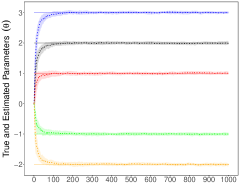
(a) Coefficients

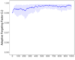
(b) Forgetting factor

Figure 2: Evolution of estimated coefficients, and the forgetting factor, $\lambda$, for a static data generating process.

Figure 2(b) illustrates the evolution of the forgetting factor, $\lambda_{t}$, through the ADAM stochastic gradient descent algorithm. The value of $\lambda_{t}$ is high throughout the simulation, and as $\hat{\theta}_{t}$ converges to $\theta_{0}$ the median value of $\lambda_{t}$ increases and the variability across simulations decreases. As the forgetting factor tends to unity, past and present examples become equally weighted and consequently parameter estimates become more accurate and less variable.

Abrupt Change

Next, we consider dynamic environments in which the coefficient vector changes at distinct time points, and remains constant in-between consecutive change points. We consider again time series of length 1000, and introduce change points at $t=100,400,700$. As in the static environment, we simulate data from a single time series of $\theta_{t}$ and create 100 time series of $y_{t}$ by different realisations of the noise term in the measurement equation, Eq (2). The time series of the coefficient vector $\theta_{t}$ is specified by $\theta_{0}=(3,2,1,-1,-2)^{\top}$ and,

$$\theta_{t}=\left\{\begin{array}[]{ll}0.5\,\theta_{t-1}&\textrm{if }t=100,\\ 1.4\,\theta_{t-1}&\textrm{if }t=400,\\ 0.7\,\theta_{t-1},&\textrm{if }t=700,\\ \theta_{t-1},&\textrm{otherwise}.\end{array}\right.$$

The specific trajectory for $\theta_{t}$ is selected because it allows a clear visualisation of the evolution of $\hat{\theta}_{t}$ at each time-step. Solid lines in Figure 3(a) depict the evolution of $\theta_{t}$ while dotted lines and shaded areas of the same colour correspond to the median estimated parameter and the associated interquartile range, respectively.

At the first change point, $t=100$, the magnitude of the change in every element of $\theta_{t}$ is the largest. Figure 3(b) shows that $\lambda_{t}$ decreases very rapidly in response to this, and by the time step $t=200$ it assumes the smallest values observed during these simulations. The minimum value of $\lambda_{t}$ observed is lower than 0.9 which implies a very aggressive forgetting of past information, or equivalently a very small effective window size. As $\hat{\theta}_{t}$ approaches $\theta_{t}$, the forgetting factor steadily increases and approaches its maximum value when the two almost coincide. This occurs right before the second change point at $t=400$. The change in $\theta_{t}$ at $t=400$ is much smaller than that at the first change point, and this is reflected in the evolution of the forgetting factor. As Figure 3(b) shows $\lambda_{t}$ decreases rapidly following the second change point but the lowest median value, which is close to 0.95, is much higher than the corresponding minimum following the first change point. Subsequently, the forgetting factor increases steadily as the estimated coefficients converge to the true values. The third change point at $t=700$ reverts $\theta_{t}$ to its value prior to the second change point. As Figure 3(b) shows the effect of this change point on $\lambda_{t}$ is very similar to the pattern observed after the second change point.

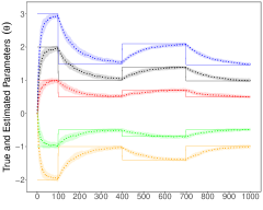
(a) Coefficients

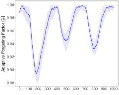
(b) Forgetting factor

Figure 3: Evolution of estimated coefficients, and the forgetting factor, $\lambda$, for a data generating process with abrupt changes.

Overall, the results depicted in Figure 3 indicate that the proposed adaptive forgetting algorithm is capable of tuning $\lambda_{t}$ effectively in the presence of change points. Following each change point AF-DLM induces a sharp decline in $\lambda_{t}$, which enables the estimated coefficients to adjust rapidly. As $\hat{\theta}_{t}$ converges to the true coefficients, which are static in-between consecutive change points, $\lambda_{t}$ increases and, if the interval between consecutive change points is sufficiently long, it approaches unity.

Gradual Drift

Finally, we consider time series in which the coefficient vector changes gradually over time. For this purpose, we simulate from the state-space model assumed by the DMA algorithm, namely Eqs. (1) to (10), with $\theta_{0}=0$. Our objective in this case is to evaluate whether the proposed adaptive forgetting method can identify the true value of $\lambda$. Note that in this case we are not able to simulate different realisations of $y_{t}$ for a single time series of $\theta_{t}$, since the state transition covariance matrix, $W_{t}$, depends on the previous realisations of the forecast error.

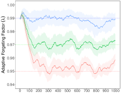
Figure 4: Evolution of $\lambda_{t}$ for time-series data sampled from the state-space model assumed by DMA for three different values of $\lambda$.

We consider three values of the forgetting factor, $\lambda\in\{0.99,0.97,0.95\}$, and for each value simulate 100 time series. In Figure 4 the dashed horizontal lines correspond to the true values of $\lambda$, while the solid lines and the shaded regions of the same colour depict the median and interquartile range of $\lambda_{t}$, respectively. As the figure shows the proposed method rapidly adjusts $\lambda_{t}$ towards the true value. After the initial adjustment period $\lambda_{t}$ fluctuates around the true value. This fluctuation is more variable for smaller values of $\lambda$, which is consistent with the model since a smaller forgetting factor implies a higher variability in the trajectory of $\theta_{t}$. Note that beyond the initial adjustment period, the median value of $\lambda_{t}$ is never more than 0.01 away from the true value. Furthermore, the interquartile range of $\lambda_{t}$ contains the true value in the vast majority of time-steps (the only exceptions occur for $\lambda=0.95$ and their duration is short).

Overall, the results on simulated time series illustrate that AF-DLM can effectively tune the value of the forgetting factor under different types of variation in the data generating process. In response to abrupt changes AF-DLM decreases $\lambda$ sharply thereby enabling the estimated coefficients to adjust rapidly. When the coefficients are static the adaptive forgetting factor tends to unity hence improving the accuracy and stability of the estimation process. In cases where the coefficients change gradually the forgetting factor fluctuates around a value that reflects the speed of drift. This concludes our empirical evaluation of the AF-DLM and in the next section we focus on the comparative evaluation of ADMA on the problem of forecasting UK regional house prices.

4 Forecasting UK Regional House Prices

For our empirical application, we employ quarterly seasonally adjusted regional house price indices for the period 1982:Q1 to 2017:Q4. The data is provided by Nationwide, the largest building society in the world and one of the largest mortgage providers in the UK. Following Nationwide’s classification, we consider 13 regional housing markets: the North, Yorkshire and Humberside, North West, East Midlands, West Midlands, East Anglia, Outer South East, Outer Metropolitan, Greater London, South West, Wales, Scotland and Northern Ireland. To transform nominal into real prices, we divide by the consumer price index (all items), obtained from the OECD Database of Main Economic Indicators, and then compute the annualised log transformation of real property price inflation as,

$$y_{r,t}=400\times\ln\left(\frac{P_{r,t}}{P_{r,t-1}}\right),\hskip 11.38092ptr=1,\dotsc,13,$$ (34)

where $P_{r,t}$ stands for the level of the real house price index of market $r$ at time $t$.

For each region in our sample, we consider eleven economic variables as potential predictors of future house price movements: four regional-level and seven national-level predictors. The variables measured at the regional level include the price-to-income ratio (which proxies for affordability), income growth, the unemployment rate, and the growth in labour force. National-level predictors consist of the real mortgage rate, the spread between yields on long-term and short-term government securities, growth in industrial production, the number of housing starts, growth in real consumption, the Credit Conditions Index (CCI) proposed by Fernandez-Corugedo and Muellbauer (2006), and a new measure of House Price Uncertainty (HPU) which we construct using the news based methodology of Baker et al. (2016). For a description of the variables, the data sources and the transformations undertaken we refer the reader to Appendix B.

From the above predictors, the first nine have been used by Bork and Møller (2015) to forecast house price movements in US metropolitan states. The last two have not been employed in a forecasting context before but may well have predictive content for future house price inflation. With regard to CCI, credit supply conditions in the UK economy, especially in the mortgage market, have changed dramatically since the 1970s. As argued by several authors, such changes were at the heart of the housing boom that preceded the Great Recession. It therefore seems natural to investigate whether an index of credit conditions may contain valuable information for forecasting. Similarly, changes in house price uncertainty impact on housing investment and real estate construction decisions (Cunningham, 2006; Banks et al., 2015; Oh and Yoon, 2019), and thus may lead to future house price movements.

In addition to macro and financial variables, there is a substantial empirical literature that documents the existence of strong spatial linkages between UK regional markets in sample (see, e.g., Drake, 1995; Meen, 1999; Cook and Thomas, 2003; Holly et al., 2010; Antonakakis et al., 2018, inter alia). To accommodate this, we incorporate in the set of potential predictors lagged property price growth in contiguous regions. The number of neighbouring regions for each of the 13 real estate markets under consideration lies in the range of one to five.

4.1 In-Sample Evidence of Structural Instability

Before proceeding to the forecasting exercise, we examine whether there is evidence of structural instability in the relationship between real house price inflation and individual house price predictors in sample. To do so, we employ two tests proposed by Chen and Hong (2012). The first is a Hausman-type ($H$) test that compares time-varying parameter estimates obtained by local linear regression to constant estimates obtain by ordinary least squares. The second is a Chow-type ($C$) test which compares the sum of squared residuals between the constant parameter and local linear regression models. The null hypothesis in both tests is that of time-invariant regression coefficients.

The $H$ and $C$ tests have a number of attractive features. First, because they impose minimal restrictions on the functional form of the time-varying parameters, they are consistent with both smooth and abrupt structural change and, from this perspective, correspond well to the AF-DLM of Section 2. Second, they require no prior information regarding the timing and the number of breaks. Third, they are asymptotically pivotal and, fourth, they do not involve trimming of the boundary region near the end points of the sample period.

Table 1: Stability Test Results

	EA		EM		GL		NI		NT		NW		OM
	$H$	$C$	$H$	$C$	$H$	$C$	$H$	$C$	$H$	$C$	$H$	$C$	$H$	$C$
Univariate Predictor Regressions
RATIO	0.0011	0.0015	0.0018	0.0019	0.0003	0.0000	0.0000	0.0000	0.0169	0.0013	0.0808	0.0322	0.0001	0.0002
GROWTH	0.0006	0.0008	0.0008	0.0000	0.0000	0.0000	0.0000	0.0000	0.0017	0.0011	0.0002	0.0000	0.0000	0.0000
UR	0.0000	0.0000	0.0003	0.0000	0.0000	0.0000	0.0018	0.0024	0.0000	0.0000	0.0000	0.0000	0.0000	0.0000
LF	0.0000	0.0000	0.0000	0.0000	0.0000	0.0000	0.0202	0.0065	0.0039	0.0020	0.0001	0.0000	0.0001	0.0000
HS	0.0000	0.0000	0.0001	0.0001	0.0000	0.0000	0.0014	0.0127	0.0052	0.0004	0.0002	0.0000	0.0000	0.0000
CONS	0.0001	0.0001	0.0001	0.0000	0.0000	0.0000	0.0002	0.0009	0.0034	0.0061	0.0001	0.0003	0.0000	0.0000
INDUS	0.0003	0.0000	0.0000	0.0000	0.0000	0.0000	0.0018	0.0023	0.0002	0.0003	0.0000	0.0000	0.0000	0.0000
RABMR	0.0004	0.0000	0.0006	0.0001	0.0000	0.0000	0.0222	0.0033	0.0015	0.0000	0.0000	0.0000	0.0000	0.0000
SPREAD	0.0000	0.0000	0.0000	0.0000	0.0000	0.0000	0.0752	0.0859	0.0000	0.0001	0.0000	0.0000	0.0000	0.0000
CCI	0.0000	0.0000	0.0027	0.0000	0.0000	0.0000	0.0000	0.0008	0.0197	0.0034	0.0028	0.0004	0.0000	0.0000
HPU	0.0001	0.0199	0.0000	0.0000	0.0000	0.0000	0.0000	0.0000	0.0012	0.0037	0.0000	0.0000	0.0000	0.0003

• Notes: The table reports wild-bootstrap $p$-values, based on $B=9999$ iterations, of the Hausman- ($H$) and Chow-type ($C$) structural stability tests of Chen and Hong (2012).

Table 2: Stability Test Results (Cont.)

	OSE		SC		SW		WM		WW		YH
	$H$	$C$	$H$	$C$	$H$	$C$	$H$	$C$	$H$	$C$	$H$	$C$
Univariate Predictor Regressions
RATIO	0.0000	0.0000	0.0037	0.0058	0.0180	0.0018	0.0181	0.0112	0.0000	0.0000	0.0043	0.0017
GROWTH	0.0000	0.0000	0.0002	0.0000	0.0002	0.0002	0.0003	0.0001	0.0023	0.0013	0.0030	0.0078
UR	0.0000	0.0000	0.0015	0.0000	0.0000	0.0000	0.0000	0.0000	0.0001	0.0000	0.0000	0.0000
LF	0.0000	0.0000	0.0012	0.0003	0.0000	0.0000	0.0006	0.0002	0.0000	0.0000	0.0059	0.0019
HS	0.0000	0.0000	0.0192	0.0357	0.0000	0.0000	0.0000	0.0000	0.0041	0.0013	0.0008	0.0009
CONS	0.0000	0.0000	0.0018	0.0048	0.0000	0.0000	0.0003	0.0000	0.0010	0.0008	0.0005	0.0016
INDUS	0.0000	0.0000	0.0000	0.0001	0.0000	0.0000	0.0000	0.0000	0.0242	0.0057	0.0002	0.0003
RABMR	0.0000	0.0000	0.0006	0.0000	0.0000	0.0000	0.0008	0.0000	0.0002	0.0000	0.0134	0.0049
SPREAD	0.0000	0.0000	0.0012	0.0004	0.0000	0.0000	0.0000	0.0000	0.0000	0.0000	0.0000	0.0000
CCI	0.0000	0.0000	0.0001	0.0003	0.0000	0.0000	0.0000	0.0000	0.0446	0.0008	0.0408	0.0066
HPU	0.0000	0.0013	0.0000	0.0010	0.0001	0.0008	0.0000	0.0014	0.0003	0.0026	0.0000	0.0003

• Notes: The table reports wild-bootstrap $p$-values, based on $B=9999$ iterations, of the Hausman- ($H$) and Chow-type ($C$) structural stability tests of Chen and Hong (2012).

Tables 1 and 2 report wild-bootstrap $p$-values of the $H$ and $C$ tests for each of the 11 house price predictors considered and for each of the 13 regions. We observe that, out of the 286 $p$-values, none exceeds 10 percent, four exceed five percent, and the vast majority lie below the one percent threshold. This strong evidence of structural instability motivates the use of dynamic econometric models for forecasting house price inflation.

4.2 Comparison of Forecast Accuracy

We begin our out-of-sample analysis by comparing the forecast accuracy of a battery of econometric models relative to the AR(1) benchmark as well as the performance of ADMA relative to each of the remaining models in the pool. This set of models consists of the DMA formulation of Dangl and Halling (2012) (abbreviated as eDMA due to the R implementation of Catania and Nonejad (2018)), two versions of the DMA of Koop and Korobilis (2012) (one with relatively slow forgetting, $\lambda=\alpha=0.99$, and another with fast forgetting $\lambda=\alpha=0.95$), a single DLM with $\lambda=0.99$ that includes all available predictors and, finally, Bayesian Model Averaging (BMA). Table 3 provides an overview of all models.

Table 3: An Overview of the Alternative Forecasting Strategies

ADMA	Adaptive Dynamic Model Averaging which uses adaptive forgetting and the aggregating algorithm of V’yugin and Trunov (2019)
eDMA	Dynamic Model Averaging which uses the grid of values $(0.90,0.91,\dotsc,0.99)$ for $\lambda$ and $\alpha=1$ (Dangl and Halling, 2012)
DMA0.99	Dynamic Model Averaging with $\lambda=\alpha=0.99$ (Raftery et al., 2010; Koop and Korobilis, 2012)
DMA0.95	Dynamic Model Averaging with $\lambda=\alpha=0.95$ (Koop and Korobilis, 2012)
BMA	Bayesian Model Averaging (Hoeting et al., 1999)
DLM0.99	A single time-varying parameter model with $\lambda=0.99$ that includes all the predictors
AR(1)	Recursive AR(1) model

Table 4 summarizes the forecasting performance of each model relative to the AR(1) benchmark over the out-of-sample evaluation period, which runs from 1995:Q1 to 2017:Q4. The second column of the table provides the realised Mean Squared Forecast Error (MSFE) of the AR(1) model for each region, while the remaining columns report the ratio of the MSFE of the competing models to that of the AR(1). Tables 5 and 6 report MFSE ratios when ADMA is set as the alternative and the benchmark model, respectively. In all three tables, a $\dagger$ indicates cases when the test of Clark and West (2007) rejects the null hypothesis of equal predictive accuracy in favour of the one-sided alternative that the competing model outperforms the benchmark at the 5% significance level.

Table 4: Summary of Forecasting Performance

(1)	(2)	(3)	(4)	(5)	(6)	(7)	(8)
Region	AR(1)	ADMA	eDMA	DMA0.99	DMA0.95	BMA	DLM0.99
East Anglia	101.05	0.80 $\dagger$	1.04	1.03	1.24	1.32	1.39
East Midlands	70.74	0.80 $\dagger$	0.79 $\dagger$	0.84 $\dagger$	0.83 $\dagger$	0.79 $\dagger$	1.44
Greater London	117.29	0.74 $\dagger$	0.79 $\dagger$	0.79 $\dagger$	0.77 $\dagger$	0.73$\dagger$	0.77 $\dagger$
Northern Ireland	292.44	0.89 $\dagger$	0.97 $\dagger$	0.92 $\dagger$	1.00	1.02	0.94 $\dagger$
North	167.39	0.72 $\dagger$	0.75 $\dagger$	0.78 $\dagger$	0.74 $\dagger$	0.69 $\dagger$	0.78 $\dagger$
North West	64.59	0.93 $\dagger$	0.92 $\dagger$	1.02	0.94 $\dagger$	0.94 $\dagger$	1.11
Outer Metropolitan	54.51	0.95$\dagger$	1.04	1.14	0.96 $\dagger$	0.95$\dagger$	1.16
Outer South East	61.84	0.92 $\dagger$	1.01	1.06	1.05	1.06	1.33
Scotland	78.18	0.94 $\dagger$	0.90 $\dagger$	0.99 $\dagger$	1.03	0.96 $\dagger$	0.99 $\dagger$
South West	60.25	0.99 $\dagger$	0.97	0.98 $\dagger$	1.15	1.13	1.58
West Midlands	53.34	0.85 $\dagger$	0.97 $\dagger$	0.95 $\dagger$	0.94 $\dagger$	0.94 $\dagger$	1.44
Wales	148.29	0.81 $\dagger$	0.79 $\dagger$	0.90 $\dagger$	0.80 $\dagger$	0.80 $\dagger$	0.87 $\dagger$
Yorkshire & Humber	91.75	0.78$\dagger$	0.79 $\dagger$	0.88 $\dagger$	0.80 $\dagger$	0.79 $\dagger$	0.82 $\dagger$

• Notes: The second column of the table reports the realised MSFE of the AR(1) model. For the remaining models, the table reports the ratio of their realised MSFE to that of the AR(1). The forecasting model with the lowest MSFE is in bold. A $\dagger$ indicates rejection of the null hypothesis of the Clark and West (2007) test at the 5% significance level.

Table 5: Forecasting Performance of ADMA Relative to Alternative Forecasting Strategies

(1)	(2)	(3)	(4)	(5)	(6)
Region	eDMA	DMA0.99	DMA0.95	BMA	DLM0.99
East Anglia	0.78 $\dagger$	0.79 $\dagger$	0.66 $\dagger$	0.61 $\dagger$	0.58 $\dagger$
East Midlands	1.02	0.96 $\dagger$	0.97 $\dagger$	1.02	0.56 $\dagger$
Greater London	0.94 $\dagger$	0.93 $\dagger$	0.96 $\dagger$	1.01	0.97 $\dagger$
Northern Ireland	0.92	0.95	0.87 $\dagger$	0.88 $\dagger$	0.94 $\dagger$
North	0.95 $\dagger$	0.91 $\dagger$	0.97 $\dagger$	1.03	0.92 $\dagger$
North West	1.01	0.91 $\dagger$	0.99	0.99	0.83 $\dagger$
Outer Metropolitan	0.92 $\dagger$	0.84 $\dagger$	0.99	1.00	0.82 $\dagger$
Outer South East	0.90 $\dagger$	0.87 $\dagger$	0.89 $\dagger$	0.86 $\dagger$	0.69 $\dagger$
Scotland	1.04	0.95 $\dagger$	0.91$\dagger$	0.98	0.94 $\dagger$
South West	1.02	1.01	0.86 $\dagger$	0.88 $\dagger$	0.63 $\dagger$
West Midlands	0.87 $\dagger$	0.89 $\dagger$	0.89 $\dagger$	0.89 $\dagger$	0.58 $\dagger$
Wales	1.02	0.89 $\dagger$	1.00	1.01	0.93 $\dagger$
Yorkshire & Humber	0.99	0.89 $\dagger$	0.98	0.99	0.96 $\dagger$

• Notes: The table reports the ratios of realised MSFEs of ADMA relative to eDMA, DMA^0.99, DMA^0.95, BMA and TVP. Figures highlighted in bold indicate that the realised MSFE of the ADMA is less than that of the alternative model. A $\dagger$ indicates rejection of the null hypothesis of the Clark and West (2007) test at the 5% significance level.

Table 6: Forecasting Performance of Alternative Forecasting Strategies Relative to ADMA

(1)	(2)	(3)	(4)	(5)	(6)
Region	eDMA	DMA0.99	DMA0.95	BMA	DLM0.99
East Anglia	1.29	1.28	1.54	1.65	1.91
East Midlands	0.98 $\dagger$	1.04	1.03	0.98 $\dagger$	1.93
Greater London	1.06	1.07	1.04	0.99	1.02
Northern Ireland	1.08	1.03	1.12	1.14	1.18
North	1.05	1.09	1.03	0.97	1.24
North West	0.99	1.10	1.01	1.01	1.22
Outer Metropolitan	1.08	1.19	1.01	1.00	1.33
Outer South East	1.10	1.16	1.14	1.16	1.55
Scotland	0.96 $\dagger$	1.05	1.09	1.02	1.12
South West	0.98 $\dagger$	0.98 $\dagger$	1.15	1.14	1.76
West Midlands	1.14	1.12	1.12	1.11	1.84
Wales	0.98	1.12	1.00	0.98	1.08
Yorkshire & Humber	1.01	1.12	1.02	1.01	1.04

• Notes: The table reports the ratios of realised MSFEs of eDMA, DMA_0.99, DMA_0.95, BMA and DLM_0.99 relative to ADMA. Figures highlighted in bold indicate that the realised MSFE of the competing forecasting strategy is less than that of ADMA. A $\dagger$ indicates rejection of the null hypothesis of the Clark and West (2007) test at the 5% significance level.

It is evident from Tables 4, 5 and 6 that ADMA performs better than all other methods. First, it is the only method that achieves a statistically significant improvement over the benchmark in all regional markets and, second, it produces on average the most accurate forecasts with a mean MSFE 15% lower than the AR(1). The second best forecasting method is eDMA. This method generates significantly more accurate forecasts than the AR(1) model in nine regional markets and achieves a 10% average improvement in MSFE relative to the benchmark. A comparison of ADMA and eDMA suggests that ADMA is more accurate in eight of the 13 regions, with this improvement being statistically significant in six cases. In contrast, eDMA performs significantly better than ADMA in only three regions. DMA with fixed forgetting also outperforms the AR(1) benchmark in the majority of cases but its performance depends critically on the choice of $\lambda$ and $\alpha$, and no choice appears to be uniformly better. ADMA generates more accurate forecasts than DMA_0.99 and DMA_0.95 in all regional property markets but one. This forecast improvement is statistically significant in 11 regions for DMA_0.99 and in nine regions for DMA_0.95. BMA achieves a lower MSFE than ADMA in four markets but in all cases the difference is very small, and only once it is found to be statistically significant. In contrast, ADMA achieves a significant improvement over BMA in five regional markets. Finally, the performance of DLM_0.99 is uniformly worse than that of ADMA, and this model outperforms the benchmark only in six regional markets. This outcome is consistent with Koop and Korobilis (2012) and Bork and Møller (2015), who argue that the use of a large number of explanatory variables can cause model over-fitting which leads to inaccurate predictions.

4.3 Best House Price Predictors Over Time and Across Regions

Having discussed forecast accuracy, we employ the estimated ADMA weights, $w_{k,t+1}$, to identify important variables for predicting future property price movements, and to investigate how the best house predictors vary over time and across regional markets. Following Koop and Korobilis (2012), for each predictor in our dataset, we scan through the set of DLMs and select those which contain the variable under consideration in their specification. The probability that ADMA assigns to this subset of models, called the posterior inclusion probability, reflects the importance of the variable in forecasting.

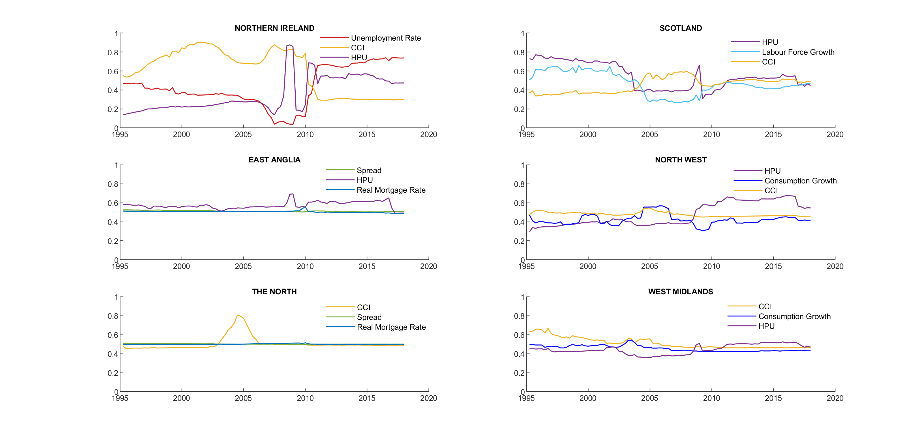
Figure 5: Posterior inclusion probabilities for the three most important predictors in the three most volatile UK regional markets (Northern Ireland, East Anglia, the North) and the three most stable markets (Scotland, North West, West Midlands)

Figure 5 displays the estimated posterior inclusion probabilities. For presentation purposes, we report results for the three most important predictors - classifying a predictor as important on the basis of its ADMA weights over the entire evaluation period- and focus on the three most volatile (Northern Ireland, East Anglia, the North) and the three most stable regional markets (Scotland, North West, West Midlands). Overall, the results in Figure 5 suggest that the best predictors differ over time and across regions.

For volatile regions, we observe that in two out of the three regions (Northern Ireland and the North), the key house price predictor during the recent boom is CCI. In Northern Ireland, which is the most volatile region in our sample, the posterior inclusion probability attached to CCI is consistently high throughout the boom phase but drops in the last part of the sample period. In the North, the CCI posterior inclusion probability increases from around 40% in 1995 to 80% in 2004 and then falls back to its original level. These findings are in line with the widely held view that changes in credit conditions were at the heart of the house price surge prior to the financial crisis.

On the other hand, house price uncertainty plays an important role in predicting future house price movements in volatile markets ahead of the house price collapse of 2008:Q3. The probability of including HPU in the forecasting models of Northern Ireland and East Anglia rises to around 90% and 70%, respectively, in 2008:Q3 and then drops following the downturn in property prices. The mortgage rate and spread are important predictors of house price inflation in East Anglia and the North, though their ADMA weights are only marginally above 0.5. With regard to the other predictive variables, we note that these are important in some volatile regions, but not in others. Perhaps the most striking example is the unemployment rate. For Northern Ireland, this variable is one of the key determinants of future property price movements in the aftermath of the house price collapse, with an ADMA weight of around 0.7 from 20011:Q1 until the end of the sample. On the contrary, for East Anglia and the North, the probability of including the unemployment rate in the predictive model is never above 0.5.

Moving on to the stable housing markets of Scotland, North West and West Midlands, we notice that credit availability and house price uncertainty are again included in the set of important predictors. In all three regions, HPU becomes the best predictor ahead of the house price collapse of 2008:Q3 and during the bust phase. While, CCI is the key determinant of property price inflation at the start of the boom phase, from the first quarter of 2004 until the end of 2005. Similarly to volatile property markets, the remaining predictors show mixed predictive ability. Overall the results of the empirical application suggest that allowing for structural instability and regional heterogeneity is crucial for forecasting UK house prices.

5 Conclusions

Dynamic model averaging (DMA) is gaining increasing attention in macroeconomic time series forecasting due to its ability to accommodate time-variation in both the parameters as well as the specification of the optimal forecasting model. In this paper we introduced a novel adaptive methodology for DMA which aims to overcome limitations of existing DMA specifications with respect to both the sequential estimation of the optimal forgetting factor for each dynamic linear model (DLM), as well as the model averaging process. Motivated by work in adaptive filtering, we proposed to optimise the forgetting factor of each DLM through a state-of-the-art stochastic gradient descent algorithm. Our simulation study illustrated that this approach can effectively approximate the optimal forgetting factor under different types of change in the data generating process, including cases in which the speed or type of change is variable over time. A further advantage of our approach is that it is computationally less demanding compared to competing DMA specifications that sequentially update the DLM forgetting factor by considering a grid of values for this parameter. Our adaptive methodology also involves a parameter-free forecast aggregation algorithm from the literature on prediction with expert advice. This allows us to obtain finite-time performance guarantees about the forecast accuracy of the DMA forecast. To the best of our knowledge no other DMA specification has this property.

We conducted an in-depth empirical evaluation of the proposed methodology on the task of forecasting UK regional house prices. Our results indicate that the adaptive DMA produces overall more accurate forecasts than competing DMA specifications. They also reveal that no single predictor is consistently chosen as the key determinant of future property price movements. Credit availability was found to be an important predictor of house price inflation for several regional markets during the boom phase of the 2000s, while house price uncertainty appeared to play an important role in predicting house price movements on the eve of the price collapse of 2008:Q3.

Appendix A Adaptive Forgetting DLM

In this appendix we derive all the derivatives necessary to compute $\frac{\partial J_{t+1}}{\partial\lambda}$. For completeness, we repeat the chain rule equation,

$$\frac{\partial J_{t+1}}{\partial\lambda}=\frac{\partial J_{t+1}}{\partial\hat{\theta}_{t}}\frac{\partial\hat{\theta}_{t}}{\partial\lambda}.$$ (A.1)

First, we introduce two equations that follow directly from the definition of DLM, and which we will need in the following derivations. Replacing the definition of the adaptive coefficient vector $A_{t}$, Eq. (19), in Eq. (18) yields the following equivalent expression for the estimator of the conditional covariance of $\theta_{t}$,

$$C_{t} =\lambda^{-1}C_{t-1}-A_{t}x_{t}^{\top}\lambda^{-1}C_{t-1}.$$ (A.2)

Combining the above with Eq. (19) yields,

$$A_{t} =C_{t}x_{t}S_{t-1}^{-1}.$$ (A.3)

We now proceed to the derivation of $\frac{\partial J_{t}}{\partial\lambda}$. Obtaining an expression for the first derivative in Eq. (2.2) is straightforward,

$$\frac{\partial J_{t+1}}{\partial\hat{\theta}_{t}}=-\hat{\varepsilon}_{t+1}x_{t+1}^{\top}.$$ (A.4)

The derivative of $\hat{\theta}_{t}$ with respect to the forgetting factor, $\frac{\partial\hat{\theta}_{t}}{\partial\lambda}$, is obtained by differentiating Eq. (17) with respect to $\lambda$,

$$\frac{\partial\hat{\theta}_{t}}{\partial\lambda} =\nabla_{\lambda}\left\{\hat{\theta}_{t-1}+A_{t}\hat{\varepsilon}_{t}\right\}$$

$$=\nabla_{\lambda}\left\{\hat{\theta}_{t-1}+C_{t}x_{t}S_{t-1}^{-1}\hat{\varepsilon}_{t}\right\}$$

$$=\frac{\partial\hat{\theta}_{t-1}}{\partial\lambda}+\frac{\partial C_{t}}{\partial\lambda}x_{t}S_{t-1}^{-1}\hat{\varepsilon}_{t}-C_{t}x_{t}S_{t-1}^{-2}\frac{\partial S_{t-1}}{\partial\lambda}\hat{\varepsilon}_{t}-C_{t}x_{t}S_{t-1}^{-1}x_{t}^{\top}\frac{\partial\hat{\theta}_{t-1}}{\partial\lambda}$$

$$=(I-C_{t}x_{t}S_{t-1}^{-1}x_{t}^{\top})\frac{\partial\hat{\theta}_{t-1}}{\partial\lambda}+\frac{\partial C_{t}}{\partial\lambda}x_{t}S_{t-1}^{-1}\hat{\varepsilon}_{t}-C_{t}x_{t}S_{t-1}^{-2}\frac{\partial S_{t-1}}{\partial\lambda}\hat{\varepsilon}_{t}$$

$$=(I-A_{t-1}x_{t}^{\top})\frac{\partial\hat{\theta}_{t-1}}{\partial\lambda}+\frac{\hat{\varepsilon}_{t}}{S_{t-1}}\left(\frac{\partial C_{t}}{\partial\lambda}x_{t}-A_{t-1}\frac{\partial S_{t-1}}{\partial\lambda}\right),$$ (A.5)

where $\frac{\partial C_{t}}{\partial\lambda}$ is the derivative of $C_{t}$, the estimator of the covariance matrix of $\theta_{t}$, with respect to $\lambda$, and $\frac{\partial S_{t-1}}{\partial\lambda}$ is the derivative of the point estimate of the observational variance at time $t-1$, $S_{t-1}$ with respect to $\lambda$. In the first and last steps of the above derivation we used Eq. (A.3).

We next need to derive expressions for $\frac{\partial C_{t}}{\partial\lambda}$ and $\frac{\partial S_{t}}{\partial\lambda}$. To this end we will need the derivative of the one-step-ahead predictive variance $Q_{t}$ with respect to $\lambda$, which we denote as $\frac{\partial Q_{t}}{\partial\lambda}$. By differentiating Eq. (13) we get,

$$\frac{\partial Q_{t}}{\partial\lambda}=\lambda^{-1}x_{t}^{\top}\frac{\partial C_{t-1}}{\partial\lambda}x_{t}-\lambda^{-2}x_{t}^{\top}C_{t-1}x_{t}+\frac{\partial S_{t-1}}{\partial\lambda}.$$

We are now able to get an expression for $\frac{\partial S_{t}}{\partial\lambda}$ by differentiating Eq. (16),

$$\frac{\partial S_{t}}{\partial\lambda}= \frac{\partial S_{t-1}}{\partial\lambda}+\frac{1}{n_{t}}\frac{\partial S_{t-1}}{\partial\lambda}\left(\frac{\hat{\varepsilon}_{t}^{2}}{Q_{t}}-1\right)$$

$$-\frac{S_{t-1}}{n_{t}}\left(\frac{2\hat{\varepsilon}_{t}x_{t}^{\top}\frac{\partial\hat{\theta}_{t-1}}{\partial\lambda}}{Q_{t}}+\frac{\hat{\varepsilon}_{t}^{2}}{Q_{t}^{2}}\frac{\partial Q_{t}}{\partial\lambda}\right).$$ (A.6)

Next we compute the derivative $\frac{\partial C_{t}}{\partial\lambda}$ by differentiating Eq. (A.2),

$$\frac{\partial C_{t}}{\partial\lambda}= \lambda^{-1}\frac{\partial C_{t-1}}{\partial\lambda}-\lambda^{-2}C_{t-1}-\frac{\partial A_{t}}{\partial\lambda}x_{t}^{\top}\lambda^{-1}C_{t-1}-$$

$$-A_{t}x_{t}^{\top}\lambda^{-1}\frac{\partial C_{t-1}}{\partial\lambda}+A_{t}x_{t}^{\top}\lambda^{-2}C_{t-1},$$ (A.7)

where $\frac{\partial A_{t}}{\partial\lambda}$ denotes the derivative of the adaptive coefficient vector at time $t$ with respect to $\lambda$. This derivative is obtained by differentiating Eq. (19) after expanding the term $Q_{t}$ that appears in the denominator by its definition in Eq. (13). In particular,

$$\frac{\partial A_{t}}{\partial\lambda} =\frac{\lambda^{-1}\frac{\partial C_{t-1}}{\partial\lambda}x_{t}}{Q_{t}}-\frac{\lambda^{-2}C_{t-1}x_{t}}{Q_{t}}-\frac{\lambda^{-1}C_{t-1}x_{t}\frac{\partial Q_{t}}{\partial\lambda}}{Q_{t}^{2}}$$

$$=\frac{1}{Q_{t}}\Bigg{\{}\lambda^{-1}\frac{\partial C_{t-1}}{\partial\lambda}x_{t}-\lambda^{-2}C_{t-1}x_{t}$$

$$\quad-A_{t}\left(\lambda^{-1}x_{t}^{\top}\frac{\partial C_{t-1}}{\partial\lambda}x_{t}-\lambda^{-2}x_{t}^{\top}C_{t-1}x_{t}+\frac{\partial S_{t-1}}{\partial\lambda}\right)\Bigg{\}}$$

$$=\frac{1}{\lambda Q_{t}}\frac{\partial C_{t-1}}{\partial\lambda}x_{t}-A_{t}\left(\frac{1}{\lambda}+\frac{1}{Q_{t}}\frac{\partial Q_{t}}{\partial\lambda}\right).$$ (A.8)

Substituting the above expression for $\frac{\partial A_{t}}{\partial\lambda}$ into the derivative $\frac{\partial C_{t}}{\partial\lambda}$ in Eq. (A),

$$\frac{\partial C_{t}}{\partial\lambda} =\lambda^{-1}\frac{\partial C_{t-1}}{\partial\lambda}-\lambda^{-2}C_{t}-\left(\lambda^{-1}\frac{\partial C_{t-1}}{\partial\lambda}x_{t}-\lambda^{-2}C_{t-1}x_{t}\right)\frac{\lambda^{-1}x_{t}^{\top}C_{t-1}}{Q_{t}}$$

$$\quad+A_{t}\left(\lambda^{-1}x_{t}^{\top}\frac{\partial C_{t-1}}{\partial\lambda}x_{t}-\lambda^{-2}x_{t}^{\top}C_{t-1}x_{t}+\frac{\partial S_{t-1}}{\partial\lambda}\right)\frac{\lambda^{-1}x_{t}^{\top}C_{t-1}}{Q_{t}}$$

$$\quad-A_{t}x_{t}^{\top}\lambda^{-1}\frac{\partial C_{t-1}}{\partial\lambda}+A_{t}x_{t}^{\top}\lambda^{-2}C_{t-1}$$

$$=\lambda^{-1}\frac{\partial C_{t-1}}{\partial\lambda}-\lambda^{-2}C_{t}-\left(\lambda^{-1}\frac{\partial C_{t-1}}{\partial\lambda}x_{t}-\lambda^{-2}C_{t-1}x_{t}\right)A_{t}^{\top}$$

$$\quad+A_{t}\left(\lambda^{-1}x_{t}^{\top}\frac{\partial C_{t-1}}{\partial\lambda}x_{t}-\lambda^{-2}x_{t}^{\top}C_{t-1}x_{t}+\frac{\partial S_{t-1}}{\partial\lambda}\right)A_{t}^{\top}$$

$$\quad-A_{t}x_{t}^{\top}\lambda^{-1}\frac{\partial C_{t-1}}{\partial\lambda}+A_{t}x_{t}^{\top}\lambda^{-2}C_{t-1}.$$ (A.9)

Substituting Eqs. (A.2) and (A.3) in the above equation and collecting terms yields,

$$\frac{\partial C_{t}}{\partial\lambda} =\lambda^{-1}\left(I-A_{t}x_{t}^{\top}\right)\frac{\partial C_{t-1}}{\partial\lambda}\left(I-x_{t}A_{t}^{\top}\right)$$

$$\quad+A_{t}\frac{\partial S_{t-1}}{\partial\lambda}A_{t}^{\top}+\lambda^{-1}C_{t}+\lambda^{-1}C_{t}x_{t}A_{t}^{\top}$$

$$=\lambda^{-1}\left(I-A_{t}x_{t}^{\top}\right)\frac{\partial C_{t-1}}{\partial\lambda}\left(I-x_{t}A_{t}^{\top}\right)$$

$$\quad+A_{t}\frac{\partial S_{t-1}}{\partial\lambda}A_{t}^{\top}+\lambda^{-1}C_{t}+\lambda^{-1}A_{t}S_{t-1}A_{t}^{\top}.$$ (A.10)

The above derivation illustrates that the derivatives of all the involved quantities can be expressed as functions of quantities involved in the update equations of the DLM, and $\frac{\partial C_{t}}{\partial\lambda}$ and $\frac{\partial S_{t}}{\partial\lambda}$, which can be estimated recursively. We are now in position to state the adaptive forgetting DLM algorithm. Algorithm 1 contains a detailed description, including the ADAM stochastic gradient descent algorithm which is used to update $\lambda$ in consecutive iterations. Although the algorithm is expressed in terms of quantities at time $t$ and $t-1$, the computations are ordered in a manner that allows us to perform all the updates by retaining a single copy of each quantity. In other words, there is no need to retain lagged values for any of the variables involved. Also note that the update equations for $\frac{\partial\hat{\theta}_{t}}{\partial\lambda}$ and $\frac{\partial C_{t}}{\partial\lambda}$ in Algorithm 1 are obtained by differentiating the update equations for $\hat{\theta}_{t}$ and $C_{t}$, respectively.

The first two inputs, $\{x_{t}\}_{t=1}^{T}$ and $\{y_{t}\}_{t=1}^{T}$, correspond to the time series of the covariates and response, respectively. The third input parameter, $g$, determines the variance of the prior distribution for $\theta$, see Eq. (5). We follow Catania and Nonejad (2018) and use as default value $g=100$. The next three inputs $\lambda_{0},\lambda^{+},\lambda_{-}$, correspond to the initial, the maximum and the minimum value of the forgetting factor. The default values for these parameters are 0.99, 0.999 and 0.9, respecively It is worth noting that bounds on the upper and lower values of the forgetting factor are employed by all algorithms that perform online tuning of this parameter (Haykin, 2002; Pavlidis et al., 2011; Anagnostopoulos et al., 2012). Finally, the last three parameters are employed by the ADAM stochastic gradient descent algorithm. The first, $\gamma$, determines the maximum step-size, while $\beta_{1}$ and $\beta_{2}$ control the exponential decay rates for the moving average estimates of the mean $m_{t}/(1-\beta_{1}^{t})$ and variance $v_{t}/(1-\beta_{2}^{t})$ of the estimated gradient $\frac{\partial\hat{\theta}}{\partial\lambda}$ over time.

Algorithm 1 Adaptive Forgetting DLM

1:$\{x_{t}\}_{t=1}^{T},\{y_{t}\}_{t=1}^{T},g=100,\lambda_{1}=0.99,\lambda^{+}=0.999,\lambda_{-}=0.9,\gamma=5\cdot 10^{-3},\beta_{1}=0.8,\beta_{2}=0.8$

2:$\hat{\theta}_{0}=0$

3:$\hat{\varepsilon}_{1}=y_{1}$

4:$C_{1}=gI$

5:$\frac{\partial C_{1}}{\partial\lambda}=0$

6:$Q_{1}=x_{1}^{\top}C_{1}x_{1}$

7:$A_{1}=C_{1}x_{1}/Q_{1}$

8:$\hat{\theta}_{1}=\hat{\theta}_{0}+\hat{\varepsilon}_{1}A_{1}$

9:$\frac{\partial\hat{\theta}_{1}}{\partial\lambda}=0$

10:$S_{1}=\frac{1}{2}\left(y_{1}^{2}+\hat{\varepsilon}_{1}^{2}/Q_{1}\right)$

11:$\frac{\partial S_{1}}{\partial\lambda}=0$

12:$n_{1}=2$

13:$m_{1}=0$ # Initialise ADAM Parameters

14:$v_{1}=0$

15:for  $t=2,\ldots,T$ do

16:   $n_{t}=n_{t-1}+1$

17:   $\hat{y}_{t}=x_{t}^{\top}\hat{\theta}_{t-1}$ # Prediction

18:   $Q_{t}=\lambda_{t-1}^{-1}x_{t}^{\top}C_{t-1}x_{t}+S_{t-1}$ # Prediction variance

19:   $\frac{\partial Q_{t}}{\partial\lambda}=\lambda_{t-1}^{-1}x_{t}^{\top}\frac{\partial C_{t-1}}{\partial\lambda}x_{t}-\lambda_{t-1}^{-2}x_{t}^{\top}C_{t-1}x_{t}+\frac{\partial S_{t-1}}{\partial\lambda}$

20:   $\hat{\varepsilon}_{t}=y_{t}-\hat{y}_{t}$ # Prediction error

21:   $\frac{\partial J_{t}}{\partial\lambda}=-\hat{\varepsilon}_{t}x_{t}^{\top}\frac{\partial\hat{\theta}_{t-1}}{\partial\lambda}$ # Derivarive of forecast error w.r.t $\lambda$

22:   $A_{t}=\lambda_{t-1}^{-1}C_{t-1}x_{t}/Q_{t}$ # Adaptive coefficient vector

23:   $\frac{\partial A_{t}}{\partial\lambda}=\lambda_{t-1}^{-1}Q_{t}^{-1}\frac{\partial C_{t-1}}{\partial\lambda}x_{t}-A_{t}\left(\lambda_{t-1}^{-1}+\frac{\partial Q_{t}}{\partial\lambda}Q_{t}^{-1}\right)$

24:   $\frac{\partial S_{t}}{\partial\lambda}=\frac{\partial S_{t-1}}{\partial\lambda}+\frac{1}{n_{t}Q_{t}}\left(\frac{\partial S_{t-1}}{\partial\lambda}\left(\hat{\varepsilon}_{t}^{2}-Q_{t}\right)-S_{t-1}\left(2\hat{\varepsilon}_{t}x_{t}^{\top}\frac{\partial\hat{\theta}_{t-1}}{\partial\lambda}+\frac{\hat{\varepsilon}_{t}^{2}}{Q_{t}}\frac{\partial Q_{t}}{\partial\lambda}\right)\right)$

25:   $S_{t}=S_{t-1}+n_{t}^{-1}S_{t-1}(\hat{\varepsilon}^{2}Q_{t}^{-1}-1)$ # Observational noise

26:   $\hat{\theta}_{t}=\hat{\theta}_{t-1}+A_{t}\hat{\varepsilon}_{t}$ # Posterior coefficient estimate

27:   $\frac{\partial\hat{\theta}_{t}}{\partial\lambda}=\frac{\partial\hat{\theta}_{t-1}}{\partial\lambda}+\hat{\varepsilon}_{t}\frac{\partial A_{t}}{\partial\lambda}-x_{t}^{\top}\frac{\partial\hat{\theta}_{t-1}}{\partial\lambda}A_{t}$

28:   $\frac{\partial C_{t}}{\partial\lambda}=(I-A_{t}x_{t}^{\top})\lambda_{t-1}^{-1}\frac{\partial C_{t-1}}{\partial\lambda}-(I+\lambda_{t-1}\frac{\partial A_{t}}{\partial\lambda}x_{t}^{\top}-A_{t}x_{t}^{\top})\lambda_{t-1}^{-2}C_{t-1}$

29:   $C_{t}=\lambda_{t-1}^{-1}C_{t-1}-A_{t}A_{t}^{\top}Q_{t}$ # Coefficient covariance matrix

30:   # ADAM Stochastic Gradient Descent ($\epsilon=10^{-8}$)

31:   $m_{t}=b_{1}m_{t-1}+(1-b_{1})\frac{\partial J_{t}}{\partial\lambda}$

32:   $v_{t}=b_{2}v_{t-1}+(1-b_{2})\left(\frac{\partial J_{t}}{\partial\lambda}\right)^{2}$

33:   $\lambda_{t}=\left[\lambda_{t-1}-\gamma m_{t}\left((1-\beta_{1}^{t})\left(\sqrt{v_{t}/(1-\beta_{2}^{t})}+\epsilon\right)\right)^{-1}\right]_{\lambda^{-}}^{\lambda^{+}}$

34:end for

Appendix B Variable Definitions and Data Sources

House Prices Real regional house price index (all houses, seasonally adjusted). Source: Nationwide.
Income Real average total household’s weekly expenditure. Source: Family Expenditure Survey (FES).
Price-to-Income Ratio Quarterly changes in the log of the ratio of house prices to income.
Income Growth Annualised quarterly changes in the log of real income.
Labour Force Growth Annualized quarterly changes in the log of the sum of unemployed and employed people. Source: Labour Force Survey (LFS).
Unemployment Rate Quarterly changes in the ratio of unemployed people to the labour force times 100. Source: LFS.
Real Mortgage Rate Quarterly changes in the real mortgage rate of building societies, adjusted for the cost of mortgage tax relief as in Muellbauer and Cameron (2006). Sources: OECD Main Economic Indicators and HM Revenue & Customs.
Spread Difference between the 10-year government bond yield and the rate of discount on 3-month treasury bills. Sources: Saint Louis FRED Economic Data and the Bank of England.
Industrial Production Growth Annualised quarterly changes in the log of total industrial production of all industries (seasonally adjusted). Source: Office for National Statistics (ONS).
Real Consumption Growth Annualised quarterly changes in the log of real final consumption expenditure of households and non-profit institutions serving households (seasonally adjusted, millions of UK sterling pounds). Source: ONS.
Housing Starts Log of the number of all permanent dwellings started in the UK. Source: Department for Communities and Local Government.
Index of Credit Conditions Designed as a linear spline function, this index is estimated using a two-equation system of secured and unsecured lending. For details about the methodology and sources of the data used in the estimation please refer to the supplementary Appendix to Pavlidis et al. (2017).
House Price Uncertainty Index Constructed using the methodology outlined in Baker et al. (2016) to proxy for economic policy uncertainty. The HPU is an index of search results from five large newspapers in the UK: The Guardian, The Independent, The Times, Financial Times and Daily Mail. We use LexisNexis digital archives of these newspapers to obtain a quarterly count of articles that contain the following three terms: ‘uncertainty’ or ‘uncertain’; ‘housing’ or ‘house prices’ or ‘real estate’; and one of the following: ‘policy’, ‘regulation’, ‘Bank of England’, ‘mortgage’, ‘interest rate’, ‘stamp-duty’, ‘tax’, ‘bubble’ or ‘buy-to-let’ (including variants like ‘uncertainties’, ‘housing market’ or ‘regulatory’). To meet the search criteria an article must contain terms in all three categories. The resulting series of search counts is then scaled by the total number of articles in the given newspaper and in the given quarter. Finally, to obtain the HPU index, we average across the five newspapers by quarter and normalise the index to a mean of 100.

References

- Aizenman and Jinjarak (2014) Aizenman, J. and Y. Jinjarak (2014). Real estate valuation, current account and credit growth patterns, before and after the 2008–9 crisis. Journal of International Money and Finance 48(Part B), 249–270.
- Almeida et al. (1999) Almeida, L. B., T. Langlois, J. D. Amaral, and A. Plakhov (1999). Parameter adaptation in stochastic optimization. In D. Saad (Ed.), Online Learning in Neural Networks, pp. 111–134. Cambridge University Press.
- Anagnostopoulos et al. (2012) Anagnostopoulos, C., D. K. Tasoulis, N. M. Adams, N. G. Pavlidis, and D. J. Hand (2012). Online linear and quadratic discriminant analysis with adaptive forgetting for streaming classification. Statistical Analysis and Data Mining 5(2), 139–166.
- Antonakakis et al. (2018) Antonakakis, N., I. Chatziantoniou, C. Floros, and D. Gabauer (2018). The dynamic connectedness of UK regional property returns. Urban Studies 55(14), 3110–3134.
- Anundsen (2015) Anundsen, A. K. (2015). Econometric regime shifts and the US subprime bubble. Journal of Applied Econometrics 30(1), 145–169.
- Baker et al. (2016) Baker, S. R., N. Bloom, and S. J. Davis (2016). Measuring economic policy uncertainty. The Quarterly Journal of Economics 131(4), 1593–1636.
- Banks et al. (2015) Banks, J., R. Blundell, Z. Oldfield, and J. P. Smith (2015). House price volatility and the housing ladder. Working Paper 21255, National Bureau of Economic Research.
- Baydin et al. (2018) Baydin, A. G., R. Cornish, D. M. Rubio, M. Schmidt, and F. Wood (2018). Online learning rate adaptation with hypergradient descent. In Sixth International Conference on Learning Representations (ICLR).
- Bork and Møller (2015) Bork, L. and S. V. Møller (2015). Forecasting house prices in the 50 states using dynamic model averaging and dynamic model selection. International Journal of Forecasting 31(1), 63–78.
- Byrne et al. (2018) Byrne, J. P., D. Korobilis, and P. J. Ribeiro (2018). On the source of uncertainty in exchange rate predictability. International Economic Review 59(1), 329–357.
- Catania and Nonejad (2018) Catania, L. and N. Nonejad (2018). Dynamic model averaging for practitioners in economics and finance: The eDMA package. Journal of Statistical Software 84(11), 1–39.
- Cesa-Bianchi and Lugosi (2006) Cesa-Bianchi, N. and G. Lugosi (2006). Prediction Learning and Games. Cambridge University Press.
- Chen and Hong (2012) Chen, B. and Y. Hong (2012). Testing for smooth structural changes in time series models via nonparametric regression. Econometrica 80(3), 1157–1183.
- Clark and West (2007) Clark, T. E. and K. D. West (2007). Approximately normal tests for equal predictive accuracy in nested models. Journal of Econometrics 138(1), 291–311.
- Clements and Hendry (1998) Clements, M. and D. Hendry (1998). Forecasting Economic Time Series. Cambridge University Press.
- Cook and Thomas (2003) Cook, S. and C. Thomas (2003). An alternative approach to examining the ripple effect in UK house prices. Applied Economics Letters 10(13), 849–851.
- Cunningham (2006) Cunningham, C. R. (2006). House price uncertainty, timing of development, and vacant land prices: Evidence for real options in seattle. Journal of Urban Economics 59(1), 1–31.
- Dangl and Halling (2012) Dangl, T. and M. Halling (2012). Predictive regressions with time-varying coefficients. Journal of Financial Economics 106(1), 157–181.
- De Rooij et al. (2014) De Rooij, S., T. Van Erven, P. D. Grünwald, and W. M. Koolen (2014). Follow the leader if you can, hedge if you must. Journal of Machine Learning Research 15(1), 1281–1316.
- Drake (1995) Drake, L. (1995). Testing for convergence between UK regional house prices. Regional Studies 29(4), 357–366.
- Fernandez-Corugedo and Muellbauer (2006) Fernandez-Corugedo, E. and J. Muellbauer (2006). Consumer credit conditions in the United Kingdom. Bank of England working papers 314, Bank of England.
- Ghysels et al. (2013) Ghysels, E., A. Plazzi, R. Valkanov, and W. Torous (2013). Forecasting real estate prices. In G. Elliott and A. Timmermann (Eds.), Handbook of Economic Forecasting, Volume 2, pp. 509 – 580. Elsevier.
- Giacomini and Rossi (2009) Giacomini, R. and B. Rossi (2009). Detecting and predicting forecast breakdowns. The Review of Economic Studies 76(2), 669–705.
- Haykin (2002) Haykin, S. S. (2002). Adaptive Filter Theory (4th ed.). Pearson Education.
- Herbster and Warmuth (1998) Herbster, M. and M. K. Warmuth (1998). Tracking the best expert. Machine Learning 32(2), 151–178.
- Hoeting et al. (1999) Hoeting, J. A., D. Madigan, A. E. Raftery, and C. T. Volinsky (1999). Bayesian model averaging: A tutorial. Statistical Science 14(4), 382–417.
- Holly et al. (2010) Holly, S., M. H. Pesaran, and T. Yamagata (2010). Spatial and temporal diffusion of house prices in the UK. IZA Discussion Papers 4694, Institute of Labor Economics (IZA).
- Kapetanios and Tzavalis (2010) Kapetanios, G. and E. Tzavalis (2010). Modeling structural breaks in economic relationships using large shocks. Journal of Economic Dynamics and Control 34(3), 417 – 436.
- Kingma and Ba (2015) Kingma, D. P. and J. L. Ba (2015). Adam: A method for stochastic optimization. In Proceedings of the 3rd International Conference on Learning Representations (ICLR).
- Koop and Korobilis (2012) Koop, G. and D. Korobilis (2012). Forecasting inflation using dynamic model averaging. International Economic Review 53(3), 867–886.
- Koop and Potter (2007) Koop, G. and S. M. Potter (2007). Estimation and forecasting in models with multiple breaks. The Review of Economic Studies 74(3), 763–789.
- Koop and Tole (2013) Koop, G. and L. Tole (2013). Forecasting the european carbon market. Journal of the Royal Statistical Society: Series A 176(3), 723–741.
- McCormick et al. (2012) McCormick, T. M., A. E. Raftery, D. Madigan, and R. S. Burd (2012). Dynamic logistic regression and dynamic model averaging for binary classification. Biometrics 68(1), 23–30.
- Meen (1999) Meen, G. (1999). Regional house prices and the ripple effect: A new interpretation. Housing Studies 14(6), 733–753.
- Muellbauer and Cameron (2006) Muellbauer, J. and G. Cameron (2006). Was there a British house price bubble? Evidence from a regional panel. Economics Series Working Papers 276, University of Oxford, Department of Economics.
- Ng and Wright (2013) Ng, S. and J. H. Wright (2013). Facts and challenges from the great recession for forecasting and macroeconomic modeling. Journal of Economic Literature 51(4), 1120–54.
- Office for National Statistics (2018) Office for National Statistics (2018). UK national accounts, the blue book: 2018. Technical report, Office for National Statistics.
- Oh and Yoon (2019) Oh, H. and C. Yoon (2019). Time to build and the real-options channel of residential investment. Journal of Financial Economics, in press.
- Paul (2018) Paul, P. (2018). The time-varying effect of monetary policy on asset prices. Review of Economics and Statistics, in press.
- Pavlidis et al. (2011) Pavlidis, N. G., D. K. Tasoulis, N. M. Adams, and D. J. Hand (2011). -perceptron: An adaptive classifier for data-streams. Pattern Recognition 44(1), 78–96.
- Pesaran et al. (2006) Pesaran, M. H., D. Pettenuzzo, and A. Timmermann (2006). Forecasting time series subject to multiple structural breaks. The Review of Economic Studies 73(4), 1057–1084.
- Raftery et al. (2010) Raftery, A. E., M. Kárný, and P. Ettler (2010). Online prediction under model uncertainty via dynamic model averaging: Application to a cold rolling mill. Technometrics 52(1), 52–66.
- Rapach and Strauss (2009) Rapach, D. E. and J. K. Strauss (2009). Differences in housing price forecastability across US states. International Journal of Forecasting 25(2), 351–372.
- Rossi (2013) Rossi, B. (2013). Advances in forecasting under instability. In Handbook of economic forecasting, Volume 2, pp. 1203–1324. Elsevier.
- Schraudolph (1999) Schraudolph, N. N. (1999). Local gain adaptation in stochastic gradient descent. In Proceedings of the International Conference on Artificial Neural Networks (ICANN), pp. 569–574.
- Stock and Watson (1996) Stock, J. H. and M. W. Watson (1996). Evidence on structural instability in macroeconomic time series relations. Journal of Business & Economic Statistics 14(1), 11–30.
- V’yugin and Trunov (2019) V’yugin, V. and V. Trunov (2019). Online aggregation of unbounded losses using shifting experts with confidence. Machine Learning 108(3), 425–444.

References

- Anagnostopoulos et al. (2012) Anagnostopoulos, C., D. K. Tasoulis, N. M. Adams, N. G. Pavlidis, and D. J. Hand (2012). Online linear and quadratic discriminant analysis with adaptive forgetting for streaming classification. Statistical Analysis and Data Mining 5(2), 139–166.
- Baker et al. (2016) Baker, S. R., N. Bloom, and S. J. Davis (2016). Measuring economic policy uncertainty. The Quarterly Journal of Economics 131(4), 1593–1636.
- Catania and Nonejad (2018) Catania, L. and N. Nonejad (2018). Dynamic model averaging for practitioners in economics and finance: The eDMA package. Journal of Statistical Software 84(11), 1–39.
- Haykin (2002) Haykin, S. S. (2002). Adaptive Filter Theory (4th ed.). Pearson Education.
- Fernandez-Corugedo and Muellbauer (2006) Fernandez-Corugedo, E. and J. Muellbauer (2006). Consumer credit conditions in the United Kingdom. Bank of England working papers 314, Bank of England.
- Pavlidis et al. (2017) Pavlidis, E., I. Paya, D. A. Peel, and A. Yusupova (2017). Exuberance in the UK regional housing markets. Technical report, Lancaster University, Department of Economics.
- Pavlidis et al. (2011) Pavlidis, N. G., D. K. Tasoulis, N. M. Adams, and D. J. Hand (2011). -perceptron: An adaptive classifier for data-streams. Pattern Recognition 44(1), 78–96.