Error bound conditions and convergence of optimization methods on smooth and proximally smooth manifolds

Abstract.

We analyse the convergence of the gradient projection algorithm, which is finalized with the Newton method, to a stationary point for the problem of nonconvex constrained optimization $\min_{x\in S}f(x)$ with a proximally smooth set $S=\{x\in\mathbb{R}^{n}:g(x)=0\},\;g:\mathbb{R}^{n}\rightarrow\mathbb{R}^{m}$ and a smooth function $f$. We propose new Error bound (EB) conditions for the gradient projection method which lead to the convergence domain of the Newton method. We prove that these EB conditions are typical for a wide class of optimization problems. It is possible to reach high convergence rate of the algorithm by switching to the Newton method.

Key words: Error bound condition, gradient projection algorithm, Newton’s method, nonconvex optimization, proximal smoothness

1. Introduction

Problems of constrained optimization on manifolds are complex because it is impossible to demand convexity-like conditions from a function defined on a manifold. One should use more flexible, in comparison with convexity, conditions for the function and for the set. Using these conditions we plan to analyse the convergence of the gradient projection algorithm (GPA) and the combined algorithm, including the GPA and the Newton method (NM). The principle is well known and can be found for example in [1], see also the bibliography in [1]. Nevertheless there are no estimates of the rate of convergence. The rate of convergence was estimated in a particular case for some proximally smooth sets in [2].

We consider the following finite-dimensional optimization problem

(1) $$\min_{\displaystyle x\in S}f(x),$$

with a proximally smooth set $S$. We shall consider $S$ in the form of the system of $m$ equations $g_{i}(x)=0,\,i=1,...,m$, or by the vector function $g:\mathbb{R}^{n}\rightarrow\mathbb{R}^{m},\,m<n$. In other words

(2) $$S=\{x\in\mathbb{R}^{n}:g(x)=0\}.$$

Further we also shall assume that the set $S$ is compact and the function $f$ is smooth.

The real Stiefel manifold $S_{n,k}$ is very important example of the set $S$ (2): $S_{n,k}=\{X\in\mathbb{R}^{n\times k}\ :\ X^{T}X=I_{k}\}$, $k\leq n$, $I_{k}$ is the $k\times k$ identity matrix.

Our aim is to find a point of minimum for the function $f$ on the set $S$ or, at least, a stationary point. We propose to use the GPA as a base method and to switch to Newton’s method in a small neighborhood of a stationary point. The latter will accelerate the convergence rate of the algorithm.

We want to recall some general difficulties for nonconvex problems:

• the metric projection is not a singleton and not continuous (as a set-valued function),

• there could be stationary points, which are not extremums,

• the gradient of a differentiable function is not a monotone operator.

We consider proximally smooth sets $S$ [3, 4] because of item (i). The metric projection on such set is a singleton for any point which is sufficiently close to the set.

The Error bound (EB) condition will be an important technical tool for the problem under consideration. EB conditions are widely spreaded in unconstrained optimization [5, 6] and recently they actively penetrate into problems of constrained optimization [2, 7, 8]. We propose to formulate the EB condition for the set of stationary points but not for the set of minimizers, see section  3.2. This condition replaces convexity assumptions for the function and for the set and gives the convergence of the method (and of the GPA in certain cases). Thus we solve question (ii).

We also consider functions with Lipschitz continuous gradient. For any function $f$ with Lipschitz continuous gradient $f^{\prime}$ with constant $L_{1}$ the function $f(x)+\frac{1}{2}L_{1}\|x\|^{2}$ is convex. This property helps us to solve difficulty (iii).

The proposed method can be used for minimization of a twice continuously differentiable functions on a smooth and proximally smooth compact manifolds without edge. We need not the Riemannian metric, geodesics and retraction with the help of the exponential mapping [9]. We shall use only the standard metric projection onto the set $S$.

The paper has the following structure.

Base results about the GPA and conditions of extremum are gathered in section  2: choice of the step-size and definition of a stationary point. Algorithm of minimization with switching from the GPA to the modified NM is described in section 3. New EB conditions are also defined in the same section. We give examples of problems with new EB conditions: minimization of a quadratic function on a sphere or on the Stiefel manifold. We introduce the notion of nondegenerate problem for (1). We prove that new EB conditions are typical, they take place for any nondegenerate problem. In contrast with the standard Newton method [10, Ch. 2, §1], [11, Ch. 1, §1.4] and some other algorithms [11, Ch. 4], [12, Ch. 8, §2] which converge locally, the proposed algorithm converges for any initial point $x_{0}\in S$ and its iterations belong generally to the set $S$.

For the convenience of readers we have collected proofs in Appendix at the end of the article.

2. Base notations and methods

Let $\mathbb{R}^{n}$ be an $n$-dimensional Euclidean space with the inner product $(x,y)$ for all $x,y\in\mathbb{R}^{n}$ and with the norm $\|x\|=\sqrt{(x,x)}$ for all $x\in\mathbb{R}^{n}$.

Further we demand twice continuous differentiability of the functions $f(\cdot),g_{i}(\cdot)$ ($f,g_{i}\in\mathcal{C}^{2}$), and Lipschitz continuity of the second derivatives $f^{\prime\prime}(\cdot),g^{\prime\prime}_{i}(\cdot)$. We treat the gradient $f^{\prime}$ etc. as a column.

Suppose that the function $f$ is Lipschitz with constant $L_{0}$, and its gradient $f^{\prime}$ is also Lipschitz with constant $L_{1}$.

Denote by

(3) $$g^{\prime}(x)=(g_{1}^{\prime}(x)\vdots g_{2}^{\prime}(x)\vdots\dots\vdots g_{m}^{\prime}(x))^{T}\in\mathbb{R}^{m\times n}$$

the Jacobi matrix for the function $g(x)$. We demand the standard full rank condition $\mathrm{rank}\,g^{\prime}(x)=m$ on the set $S$.

Assume that the manifold $S$ is compact and without edge. .

Denote by $T_{x}$ the tangent subspace at the point $x\in S$. It is characterized with the help of the Jacobi matrix (3) by the formula $T_{x}=\{v\in\mathbb{R}^{n}:g^{\prime}(x)v=0\}$.

The metric projection of a point $x\in\mathbb{R}^{n}$ onto a set $Q\subseteq\mathbb{R}^{n}$ is defined as follows

$$P_{Q}(x)=\{y\in Q:\|x-y\|=\rho(x,Q)\},$$

where $\rho(x,Q)=\inf_{y\in Q}\|x-y\|$ is the distance function.

We shall use vertical stacking of column vectors: $[a,b]=(a^{T},b^{T})^{T}$. The same notations will be applied for matrices $a$, $b$ of particular sizes. For a number $t>0$ we denote by $\lceil t\rceil$ the minimal natural number with $t\leq\lceil t\rceil$.

The metric projecting operator onto the tangent subspace $T_{x}$ is given by the matrix [12, Ch. 7, §2, Formula (7)]

$$P_{T_{x}}=I_{n}-g^{\prime T}(x)(g^{\prime}(x)g^{\prime T}(x))^{-1}g^{\prime}(x)=I_{n}-g^{\prime T}(g^{\prime}g^{\prime T})^{-1}g^{\prime},$$

the metric projection of a point $y\in\mathbb{R}^{n}$ onto a subspace $T_{x}$ is denoted by $P_{T_{x}}y$. The metric projecting operator $P_{T_{x}}$ is defined for all $x\in S$ by the full rank condition for matrix (3). We shall omit the dependence of an expression on argument if this dependence is obvious from a context.

For a set $S\subset\mathbb{R}^{n}$ and a number $R>0$ define the set

$$U_{S}(R)=\{x\in\mathbb{R}^{n}:0<\rho(x,S)<R\}$$

that is a layer (or ”tube”) around the set $S$.

An important requirement for the set $S$ in our work is its proximal smoothness (also known as prox-regularity or weak convexity), that is characterized by constant of proximal smoothness $R>0$.

Definition 1 ([3, 4]).

A closed set $S\subset\mathbb{R}^{n}$ is called proximally smooth with constant $R$ if the distance function $\rho(x,S)$ is continuously differentiable on $U_{S}(R)$.

Existence, uniqueness of $P_{S}x$ for all $x\in U_{S}(R)$ and continuity of the mapping $U_{S}(R)\ni x\to P_{S}x$ in a real Hilbert space are equivalent conditions for proximal smoothness of the set $S$ with constant $R$. In other words the set $S$ has the Chebyshev layer of size $R$.

For a point $x$ of a proximally smooth set $S$ the cone of proximal normals (or simply — normal cone) is defined as

$$\mathcal{N}(S,x)=\big{\{}p\in\mathbb{R}^{n}:\exists t>0,P_{S}(x+tp)=\{x\}\big{\}}.$$

This cone coincides with any other cone to the proximally smooth set $S$ at the point $x\in S$ (in particular with cones of Clarke and Bouligand) [13, 14]. For our situation, when $S$ is given by the system (2), the normal cone coincides with the orthogonal subspace to the tangent subspace $T_{x}$, i.e. $\mathcal{N}(S,x)=\{g^{\prime}(x)^{T}w:w\in\mathbb{R}^{m}\}$.

It is obvious that the Euclidean sphere of radius $R$ is proximally smooth with constant $R$.

Example 1 ([3]).

Suppose that $g:\mathbb{R}^{n}\rightarrow\mathbb{R}^{1}$, $g$ is a Lipschitz function with constant $L_{g}$ and there exists $\ell>0$ such that for any $x\in S$ we have $\|g^{\prime}(x)\|\geq\ell$. Then the set $S=\{x\in\mathbb{R}^{n}:g(x)=0\}$ is proximally smooth with constant $R=\ell/L_{g}$.

Sometimes one can calculate constant of proximal smoothness using the supporting principle for proximally smooth sets, see [15].

Proposition 1.

The Stiefel manifold $S_{n,k}=\{X\in\mathbb{R}^{n\times k}\ :\ X^{T}X=I_{k}\}$ of any dimensions is proximally smooth with constant $R=1$. This constant is the largest possible. See the proof in section 5.1 of the Appendix.

2.1. Stationary conditions

For the problem (1) with a proximally smooth set $S$ points of minimum are characterized by the next necessary condition: the anti-gradient $-f^{\prime}(x)$ at such point $x\in S$ belongs to the normal cone $\mathcal{N}(S,x)$ [2, Appendix 5.1]. We shall call such point stationary and denote their set by

$$\Omega=\{x\in S:-f^{\prime}(x)\in\mathcal{N}(S,x)\}.$$

If the set is given by the system (2), the stationary condition is equivalent to the equality $P_{T_{x}}f^{\prime}(x)=0$ (or $\|P_{T_{x}}f^{\prime}(x)\|=0$).

Consider the Lagrange function with the Lagrange multiplier $\lambda\in\mathbb{R}^{m}$:

$$f(x)+\sum_{i=1}^{m}\lambda_{i}g_{i}(x).$$

The stationary condition can be written with the help of derivative of the Lagrange function with respect to the extended variable $z=[x,\lambda]\in\mathbb{R}^{n+m}$, i.e. in the form $F(z)=0$, where

(4) $$F(z)=F(x,\lambda)=\begin{bmatrix}f^{\prime}(x)+g^{\prime}(x)^{T}\lambda\\ g(x)\end{bmatrix}.$$

The Hessian matrix of the Lagrange function coincides with $F^{\prime}(z)$ and has the form

(5) $$F^{\prime}(z)=\begin{bmatrix}f^{\prime\prime}(x)+(g^{\prime}(x)^{T})^{\prime}_{x}\lambda&g^{\prime}(x)^{T}\\ g^{\prime}(x)&0\end{bmatrix}=\begin{bmatrix}f^{\prime\prime}(x)+\sum_{i=1}^{m}\lambda_{i}g^{\prime\prime}_{i}(x)&g^{\prime}(x)^{T}\\ g^{\prime}(x)&0\end{bmatrix}.$$

Note some relationship between the derivative of the Lagrange function at the point $[x,\lambda]$ and the metric projection $P_{T_{x}}f^{\prime}(x)$ for a point $x\in S$. For any $x\in S$ define $\lambda_{x}$ by the formula

(6) $$\lambda_{x}=\arg\min_{\lambda}\|F(x,\lambda)\|=\arg\min_{\lambda}\|f^{\prime}(x)+g^{\prime}(x)^{T}\lambda\|=-(g^{\prime}g^{\prime T})^{-1}g^{\prime}f^{\prime}.$$

We get the equality $f^{\prime}+g^{\prime T}\lambda_{x}=(I-g^{\prime T}(g^{\prime}g^{\prime T})^{-1})f^{\prime}=P_{T_{x}}f^{\prime}$. Note also that $\|F(x,\lambda_{x})\|=\|P_{T_{x}}f^{\prime}\|$. The variable $\lambda_{x}$ depends on $x$. We shall use the notation

$$F_{x}(x)\doteq F(x,\lambda_{x})=P_{T_{x}}f^{\prime}(x)$$

to distinguish the functions $F(z)$ and $F(x,\lambda_{x})$.

Further we shall use the notation $F^{\prime}(x,\lambda_{x})$ that means

(7) $$F^{\prime}(x,\lambda_{x})\doteq F^{\prime}([x,\lambda_{x}])\equiv F^{\prime}(z)\big{|}_{z=[x,\lambda_{x}]}.$$

Notice that the last expression is not a derivative of the function $F_{x}(x)$ on $x$. By the Lipschitz condition for $g^{\prime\prime}$ and $f^{\prime\prime}$ the function $F^{\prime}(x,\lambda_{x})$ is also Lipschitz in a compact neighborhood of $S$ with some constant $L_{1,Fx}$ .

2.2. The gradient projection algorithm

Consider some results about convergence of the GPA

(8) $$x_{k+1}=P_{S}(x-\gamma f^{\prime}(x_{k})).$$

for a proximally smooth set $S$ and a function $f(\cdot)$ with Lipschitz continuous gradient [2].

The idea of applying the GPA for nonconvex problem is the next one. Let $x_{k}\in S$. Then we can choose the step-size $\gamma$ with the property $x_{k}-\gamma f^{\prime}(x_{k})\in U_{S}(R)\cup S$. Projection $P_{S}(x_{k}-\gamma f^{\prime}(x_{k}))$ exists and it is unique by the definition of proximally smooth set. Next, we can adopt the step-size in such way that the sequence $f(x_{k})$ will be monotonically decreasing.

Theorem 1 ([2, Theorem 1]).

Suppose that $S$ is a proximally smooth set with constant $R$ and $x_{0}\in S$ is a starting point. Assume that a function $f:\mathbb{R}^{n}\to\mathbb{R}$ is Lipschitz with constant $L_{0}$, and its gradient is also Lipschitz with constant $L_{1}$. Then for any fixed step-size $0<\gamma<\min\{\frac{1}{L_{1}},\frac{R}{L_{0}}\}$ the GPA (8) converges to the set of stationary points $\Omega$, i.e. $\lim\limits_{k\to\infty}\rho(x_{k},\Omega)=0$. Moreover,

$$f(x_{k+1})\leq f(x_{k})-\frac{1}{2}\Big{(}\frac{1}{\gamma}-L_{1}\Big{)}\|x_{k+1}-x_{k}\|^{2}.$$

Note that we can estimate the number of steps which is necessary for finding a stationary point with any a priori precision.

Corollary 1.

Suppose that under conditions of Theorem 1 we know the value $\Delta f=f(x_{0})-\inf_{x\in S}f(x)$, and the set $S$ is given by the system (2). Then for any $\varepsilon>0$ we can find a natural number $i:0\leq i\leq\left\lceil\frac{2\Delta f(1+\gamma L_{1})^{2}}{\varepsilon^{2}\gamma(1-\gamma L_{1})}\right\rceil$ with $\|P_{T_{x_{i}}}f^{\prime}(x_{i})\|\leq\varepsilon$.

The proof of the Theorem and Corollary can be found in section 5.2 of the Appendix.

Finding the metric projection of a point onto the set is an important part of the gradient projection algorithm. If the set has simple structure then the metric projection can be easily found, e.f. for Euclidean sphere or the Stiefel manifold, see Proposition 3 in section 5.1 of the Appendix.

In paper [2, algorithm GPA2] we consider an algorithm for finding some easily computing quasi-projection instead of the metric projection for the case of one equation $g:\mathbb{R}^{n}\rightarrow\mathbb{R}$.

2.3. The Newton method

Now we formulate sufficient conditions for convergence of the Newton method for the equation $F(z)=0$. We shall assume for simplicity that the function $F(z)$ is continuously differentiable everywhere.

Proposition 2 ([16, Theorem X.4.1], see also [10, Ch. 2, §1], [11]).

Suppose that the derivative $F^{\prime}(z)$ is Lipschitz continuous with constant $L_{1,F}$, the matrix $F^{\prime}(z_{0})$ is invertible at the point $z_{0}=[\widehat{x}_{0},\lambda_{0}]$ and the condition

(9) $$L_{1,F}\,\|F^{\prime}(\widehat{x}_{0},\lambda_{0})^{-1}F(\widehat{x}_{0},\lambda_{0})\|\cdot\|F^{\prime}(\widehat{x}_{0},\lambda_{0})^{-1}\|<\frac{1}{4}$$

holds. Then the modified Newton method (11) converges to a solution $z=z^{*}=[x_{*},\lambda_{*}]$ of the equation $F(z)=0$. Moreover $z^{*}$ is a unique solution in the ball with centerpoint $z_{0}=[\widehat{x}_{0},\lambda_{0}]$ and radius $r=Kt_{0}$. Here we have $K=\|F^{\prime}(z_{0})^{-1}F(z_{0})\|$, and $t_{0}\in(0,2]$ is the smaller root of the equation $ht^{2}-t+1=0$, where $h=L_{1,F}K\|F^{\prime}(z_{0})^{-1}\|$.

Besides, a linear rate of convergence takes place for iterations of the modified Newton method:

$$\|\widehat{x}_{k}-x_{*}\|\leq 2^{1-k}\|F^{\prime}(\widehat{x}_{0},\lambda_{0})^{-1}F(\widehat{x}_{0},\lambda_{0})\|\leq 2^{1-k}\|F^{\prime}(\widehat{x}_{0},\lambda_{0})^{-1}\|\cdot\|F(\widehat{x}_{0},\lambda_{0})\|$$

and $[\widehat{x}_{k},\lambda_{k}]\in B_{r}(z_{0})$. Note that it’s sufficient to require Lipschitz continuity of $F^{\prime}(z)$ on the ball $B_{2K}(z_{0})$.

3. Main results

3.1. Combined algorithm: the GPA and the NM

We shall assume that we have information about Lipschitz constant $L_{0}$ of the function $f$ and Lipschitz constant $L_{1}$ of the gradient $f^{\prime}$. Suppose also that we know constant of proximal smoothness $R$ for the set $S$.

The next Algorithm depends on some real positive constant $C>0$, we shall specify its value below.

Combined algorithm: GPA + NM

1. Starting conditions and parameters: Given constant $C>0$.
   Choose arbitrarily $x_{0}\in S=\{x\in\mathbb{R}^{n}:g(x)=0\}$. Put $k=0$ and take $0<\gamma<\min\{\frac{1}{L_{1}},\frac{R}{L_{0}}\}$.

2. Gradient projection algorithm, GPA:
   Do (8), increasing $k$:

   $$x_{k+1}=P_{S}(x_{k}-\gamma f^{\prime}(x_{k})).$$

   In the case

   (10) $$\|P_{T_{x_{k}}}f^{\prime}(x_{k})\|<C,$$

   (or in the case (12)) go to Step 2.

3. Preparation for the NM:
   Define the initial point $\widehat{x}_{0}=x_{k}$, $\lambda_{0}=\lambda_{\widehat{x}_{0}}=-(g^{\prime}(\widehat{x}_{0})g^{\prime}(\widehat{x}_{0})^{T})^{-1}g^{\prime}(\widehat{x}_{0})f^{\prime}(\widehat{x}_{0})$, put $k=0$.

4. Modified Newton method, NM:
   Do steps of the modified NM for the equation $F(z)=F(\widehat{x},\lambda)=0$, increasing $k$:

   (11) $$\begin{array}[]{l}\begin{bmatrix}\widehat{x}_{k+1}\\ \lambda_{k+1}\end{bmatrix}=\begin{bmatrix}\widehat{x}_{k}\\ \lambda_{k}\end{bmatrix}-F^{\prime}\Big{(}\begin{bmatrix}\widehat{x}_{0}\\ \lambda_{0}\end{bmatrix}\Big{)}^{-1}F\Big{(}\begin{bmatrix}\widehat{x}_{k}\\ \lambda_{k}\end{bmatrix}\Big{)}=\\ \!\!\!\!\!\!\!\!\!\!\!\!\!\!\!=\begin{bmatrix}\widehat{x}_{k}\\ \lambda_{k}\end{bmatrix}-\begin{bmatrix}f^{\prime\prime}(\widehat{x}_{0})+\sum_{i=1}^{m}(\lambda_{k})_{i}g_{i}^{\prime\prime}(\widehat{x}_{0})&g^{\prime}(\widehat{x}_{0})^{T}\\ g^{\prime}(\widehat{x}_{0})&0\end{bmatrix}^{-1}\begin{bmatrix}f^{\prime}(\widehat{x}_{k})+g^{\prime}(\widehat{x}_{k})^{T}\lambda_{k}\\ g(\widehat{x}_{k})\end{bmatrix}.\end{array}$$

   Algorithm should be stopped with the help of some stop criteria, e.g. after a given number of steps and so on, see further.

The value $C$ is a nontrivial parameter of the Algorithm. Its calculation requires information about some additional constants, see section 3.

We want to pay attention on some peculiarities of the Algorithm.

1. Firstly, at the initial step (GPA) the sequence $x_{k}$ belongs to the manifold $S$. Condition $\gamma<R/L_{0}$ guarantees the inclusion $x_{k}-\gamma f^{\prime}(x_{k})\in S\cup U_{S}(R)$ and uniqueness of the metric projection. Another condition $\gamma<1/L_{1}$ guarantees that the sequence $f(x_{k})$ is monotonically decreasing, see the proof of Theorem 1 in section 5.2 of the Appendix. The maximum number of steps in this phase is also explicitly estimated there.

2. We can use a simpler condition for switching the GPA phase to the NM phase instead of condition (10), namely

   (12) $$\|x_{k}-x_{k-1}\|\leq\frac{\gamma}{1+\gamma L_{1}}C,\;k\geq 1.$$

   This condition needs computing of a simple value $\|x_{k}-x_{k-1}\|$ instead of $P_{T_{x_{k}}}f^{\prime}(x_{k})$. The admissibility of this condition follows from the estimate $\|x_{k}-x_{k-1}\|(\frac{1}{\gamma}+L_{1})\geq\|P_{T_{x_{k}}}(f^{\prime}(x_{k}))\|$, inequality (21) and the limit $\|x_{k}-x_{k-1}\|\rightarrow_{k\to\infty}0$ (see the proof of Corollary 1 in section 5.2 of the Appendix).

3. We use the modified NM in the second phase. It needs a unique computing of the inverse matrix $F^{\prime}(\widehat{x}_{0},\lambda_{0})^{-1}$. The points $\widehat{x}_{k}\in\mathbb{R}^{n}$ do not necessarily belong to the set $S$ and $\lambda_{k}$ is an independent variable.

The main criterion for stopping the Algorithm (the NM phase) is the inequality

$$\|P_{T_{\widehat{x}_{k}}}f^{\prime}(\widehat{x}_{k})\|\leq\varepsilon,$$

or estimate for the distance to the set of stationary points

$$\rho(\widehat{x}_{k},\Omega)\leq\varepsilon,$$

for some $\varepsilon>0$. The last is achieved after given number of steps for the NM, this number can be determined if appropriate constants are known.

The fulfillment of switching condition (10) or (12) for any $C>0$ is guaranteed by Theorem 1 about convergence of the GPA on a proximally smooth set and by Corollary 1.

Next consider the conditions that provide the convergence of the NM at the second phase of the Algorithm.

3.2. Nondegenerate problems and error bound conditions

Definition 2.

We shall call the problem (1) with $f,g\in\mathcal{C}^{2}$ nondegenerate, if for all stationary points $x_{*}\in\Omega$ the matrix $F^{\prime}(x_{*},\lambda_{x_{*}})$ is invertible. Norms of all inverse matrices are bounded from above by a value $\sigma_{0}>0$:

(13) $$\|F^{\prime}(x_{*},\lambda_{x_{*}})^{-1}\|\leq\sigma_{0},\;\;\forall x_{*}\in\Omega.$$

This definition allows to use the NM in neighborhoods of stationary points, see Lemma 3 below.

Lemma 1.

If the set $S$ is compact and the problem (1) is nondegenerate then the number of stationary points is finite, $\Omega=\{x_{j}\}_{j=1}^{J}$.

The proof can be found in section 5.3 of the Appendix.

The next important definition characterizes relationship between stationary points and $P_{T_{x}}f^{\prime}(x)$ at any point $x\in S$.

Definition 3.

We shall say that problem (1) satisfies the tangent Error Bound condition (or tEB), if there exists a positive value $\mu>0$ with

(14) $$\mu\,\rho(x,\Omega)\leq\|P_{T_{x}}f^{\prime}(x)\|=\|F_{x}(x)\|,\;\;\forall x\in S.$$

For a point $x\in S$ and $\gamma>0$ denote by $\mathcal{G}_{\gamma}(x)=\frac{x-P_{S}(x-\gamma f^{\prime}(x))}{\gamma}$ the gradient mapping at the point $x$ for problem (1) [17]. It is clear that the gradient mapping is related with one step of the GPA.

Definition 4.

We shall say that problem (1) satisfies the gradient Error Bound condition (or gEB) with constant $\nu>0$, if there exists $\gamma_{0}>0$ such that for all $0<\gamma<\gamma_{0}$ and for all $x\in S$ we have

$$\nu\rho(x,\Omega)\leq\|\mathcal{G}_{\gamma}(x)\|.$$

Definition 4 was formulated (without gEB notation) in the paper [19].

By the proof of Proposition 4 (section 5.2 of the Appendix) in the case of smooth and proximally smooth manifold the tEB condition entails the gEB condition with constant $\nu=\frac{\mu}{1+L_{1}\gamma_{0}+\mu\gamma_{0}}$ and $\gamma_{0}=\min\{\frac{1}{L_{1}},\frac{R}{L_{0}}\}$. Conditions tEB and gEB are equivalent in the case of smooth and proximally smooth manifold $S$. The proof is bulky and we omit it.

In contrast with Error Bound conditions in unconstrained optimization

$$\|f^{\prime}(x)\|\geq\mu\,\rho(x,X_{\min}),\;\;X_{\min}=\mathop{\mathrm{Arg}}\min_{x\in\mathbb{R}^{n}}f(x),$$

or equivalent Lezanski-Polyak-Lojasiewicz condition [5], we use the distance from a point $x\in S$ to the set of stationary points $\Omega$ and the value $\|P_{T_{x}}f^{\prime}(x)\|$ instead of $\|f^{\prime}(x)\|$.

Consider few examples.

Example 2.

One can explicitly calculate constant $\mu$ in the tEB condition for a quadratic form on the unit Euclidean sphere.

Lemma 2.

The tEB condition fulfills with constant

$$\mu=\min_{i\neq j}|\lambda_{i}-\lambda_{j}|$$

for a quadratic form $f(x)=(Ax,x)$, $A=A^{T}$, with different eigenvalues of the matrix $A$ ($\lambda_{1}<\lambda_{2}<...<\lambda_{n}$), on the unit sphere $\{x\in\mathbb{R}^{n}:\|x\|=1\}$.

The proof can be found in section 5.4 of the Appendix.

Example 3.

A quadratic form satisfies the tEB condition on the Stiefel manifold $S_{n,k}=\{X\in\mathbb{R}^{n\times k}:X^{T}X=I_{k}\}$ [8, Corollary 1]. This fact generalizes Lemma 2.

If problem (1) is nondegenerate then the tEB condition holds.

Theorem 2.

If problem $\eqref{eq:main}$ is nondegenerate, then the tEB condition is fulfilled with some constant $\mu>0$.

The proof can be found in section 5.5 of the Appendix.

If we demand additionally thrice continuous differentiability of all functions then, by Taylor’s formula with the Lagrange form of the remainder, one can estimate radius $r$ and constant $\mu$ in the tEB condition in Formula (27) via Lipschitz constants.

We want to pay attention that the gEB condition holds under conditions of Theorem 2 by Proposition 4. Suppose that $\Omega$ is the set of global minima from the set $S\cap\{x\ :\ f(x)\leq f(x_{0})\}$, and $x_{0}\in S$ is a starting point for the GPA. From [19] we get that the GPA converges to some element of the set $\Omega$ with linear rate. Also in the case when the tEB condition is valid, we immediately get linear convergence of GPA, see [2, Section 3.4].

Finally note that condition of non-degeneracy for problem $\eqref{eq:main}$ is not necessary for fulfillment of the tEB condition. Assume that the function $x\to\lambda_{x}$ is continuously differentiable in a neighborhood of the set $S$ of the form $U_{S}(\delta)$, $\delta>0$, and there exists a number $\mu>0$ such that for any point $x_{*}\in\Omega$ the next condition holds

$$\left\|F^{\prime}_{z}(x_{*},\lambda_{x_{*}})\left(\begin{array}[]{c}I_{n}\\ \lambda_{x}^{\prime}|_{x=x_{*}}\end{array}\right)h\right\|\geq\mu\|h\|,\quad\forall h\in T_{x_{*}}\subset\mathbb{R}^{n}.$$

Then the tEB condition holds in problem (1). The proof repeats the proof of Theorem 2. We shall not discuss this approach for proving the tEB condition because we need existence of the inverse matrix $F^{\prime}(x,\lambda_{x})$, for any $x\in\Omega$, in our situation.

3.3. Convergence of the Algorithm

Lemma 3.

Suppose that $f,g_{i}\in\mathcal{C}^{2}$, the function $\lambda_{x}$ is defined in (6), the function $F^{\prime}(x,\lambda_{x})$, is defined in (7) and is Lipschitz continuous on $S$ with constant $L_{1,Fx}$: $\|F^{\prime}(x,\lambda_{x})-F^{\prime}(y,\lambda_{y})\|\leq L_{1,Fx}\|x-y\|$ forall $x,y\in S$.

Then for any $\beta\in[0,1)$ the next estimate

$$\|F^{\prime}(x,\lambda_{x})\|\leq\frac{\sigma_{0}}{1-\beta},\quad\forall x\in S:\;\rho(x,\Omega)\leq\frac{\beta}{\sigma_{0}L_{1,Fx}}$$

takes place.

The proof can be found in section 5.6 of the Appendix.

Gathered together the above mentioned results we obtain the theorem about the convergence of the considered combined algorithm. Recall that $\gamma$ is a fix step-size in the GPA (1st phase) and $\Delta f=f(x_{0})-\min_{x\in S}f(x)$ is the fluctuation of the function.

Theorem 3.

Let $\Omega=\{x_{j}\}_{j=1}^{J}$ be the set of stationary points in problem (1), $\Sigma=\{[x,\lambda_{x}]\ :\ x\in\Omega\}$. Assume that problem (1) is nondegenerate and the tEB condition holds with constant $\mu$ (14). Suppose that in $d$-neighborhood $U_{\Omega}(d)$ of the set $\Omega$ the function $S\ni x\to\lambda_{x}$ is Lipschitz continuous with constant $L_{\lambda}$ and the function $S\ni x\to F^{\prime}(x,\lambda_{x})$ is Lipschitz continuous with constant $L_{1,Fx}$. Suppose that the function $F^{\prime}(z)$ is Lipschitz continuous with constant $L_{1,F}$ on the set $U_{\Sigma}(2r)$ for $r=d\sqrt{1+L_{\lambda}^{2}}$. Let $\sigma_{0}>0$ and $\beta\in(0,1)$ be such constants that estimate (13) holds, $\beta\leq L_{1,Fx}\sigma_{0}d$ and

(15) $$\frac{1-\beta}{2\sigma_{0}L_{1,F}}\leq r.$$

Then for any point $x_{0}\in S$ the Algorithm with the switching condition

(16) $$\|P_{T_{x}}f^{\prime}(x)\|\leq C=\min\Big{\{}\frac{\mu\beta}{L_{1,Fx}\sigma_{0}},\;\frac{(1-\beta)^{2}}{4L_{1,F}\sigma_{0}^{2}}\Big{\}},$$

or with another condition (12) $\|x_{k}-x_{k-1}\|\leq\frac{\gamma}{1+\gamma L_{1}}C$, converges to some stationary point $x_{*}\in\Omega$. We need no more than

$$N(\varepsilon)=N_{1}(C)+N_{2}(\varepsilon)=\left\lceil\frac{2\Delta f(1+\gamma L_{1})^{2}}{C^{2}\gamma(1-\gamma L_{1})}\right\rceil+\Big{\lceil}\log_{2}\Big{(}\frac{C\sigma_{0}}{\varepsilon(1-\beta)}\Big{)}\Big{\rceil}+1$$

steps of the Algorithm to achieve the inequality $\rho(x_{k},\Omega)\leq\varepsilon$. In particular, we need $N_{1}(C)$ steps of the GPA and $N_{2}(\varepsilon)$ steps of the modified NM.

The proof can be found in section  5.7.

Note that the first phase of the Algorithm, the GPA, is more difficult from computational point of view. One can minimize the number of steps for the GPA, choosing the step-size $\gamma$ and minimizing $N_{1}(C)$ as function of $\gamma$. The optimal value is

$$\gamma^{*}=\min\Big{\{}\frac{1}{3L_{1}},\frac{R}{L_{0}}\Big{\}}.$$

4. Acknowledgements

The work was supported by Russian Science Foundation (Project 16-11-10015).

The authors are greatful to B. T. Polyak for useful comments and suggestions.

5. Appendix: proofs.

5.1. Proof of Proposition 3

Proposition 3.

The Stiefel manifold $S_{n,k}$ is proximally smooth set with constant $R=1$ for all $n,k$, $n\geq k$.

Proof.

Proximal smoothness of the Stiefel manifold $\mathcal{S}_{n,k}=\{X\in\mathbb{R}^{n\times k}:X^{T}X=I_{k}\}$, $k\leq n$, with constant of proximal smoothness $R=1$ follows from the result about explicit form for the metric projection onto the Stiefel manifold [18, Proposition 7]:

$$P_{\mathcal{S}_{n,k}}(X)=UI_{k,n}V^{T},\;\;\forall X=U\Sigma V^{T}:\;\;\rho(X,\mathcal{S}_{n,k})<1.$$

For the set $\{X\in\mathbb{R}^{n\times k}:\rho(X,\mathcal{S}_{n,k})<1\}$ the metric projection is a singleton. Here $U,V$ are orthogonal matrices of a singular values decomposition for matrix $X$, $I_{k,n}=[I_{k},0]\in\mathbb{R}^{n\times k}$. The distance between matrices is understood in the Frobenius metric $\rho(X,Y)=\|X-Y\|=\left(\mbox{\rm trace\, }(X-Y)^{T}(X-Y)\right)^{1/2}$.

From upper smicontinuity of the metric projection in finite dimensional space $R^{n\times k}$ [10, Ch. 3, §1, Proposition 23] and its uniqueness we obtain that the function $U_{\mathcal{S}_{n,k}}(1)\ni X\rightarrow P_{\mathcal{S}_{n,k}}X$ is continuous.

Finally, constant of proximal smoothness can not exceed 1. For the point (matrix) $X_{0}=[0,e_{2},e_{3},...,e_{k}]\in\mathbb{R}^{n\times k}$ with $\rho(X_{0},\mathcal{S}_{n,k})=1$ there exists at least two metric projections onto the Stiefel manifold: $X_{0,-}=[-e_{1},e_{2},e_{3},...,e_{k}]$ and $X_{0,+}=[e_{1},e_{2},e_{3},...,e_{k}]$. ∎

5.2. Proof of Theorem 1, Corollary 1 and Proposition 4

Proof of Theorem 1.

For a natural $k$ define the functions

$$\psi_{k}(x)=f(x_{k})+(f^{\prime}(x_{k}),x-x_{k})+\frac{1}{2\gamma}\|x-x_{k}\|^{2}.$$

By Lipschitz continuity of the gradient $f^{\prime}$ we have

$$f(x_{k})+(f^{\prime}(x_{k}),x-x_{k})+\frac{L_{1}}{2}\|x-x_{k}\|^{2}\geq f(x),\quad\forall x\in\mathbb{R}^{n}\qquad\mbox{\rm and}$$

(17) $$\psi_{k}(x)\geq f(x)+\frac{1}{2}\Big{(}\frac{1}{\gamma}-L_{1}\Big{)}\|x-x_{k}\|^{2},$$

for all $x\in\mathbb{R}^{n}$.

By the conditions $\gamma<\frac{R}{L_{0}}$, $x_{k}\in S$, we get $x_{k}-\gamma f^{\prime}(x_{k})\in S\cup U_{S}(R)$. Indeed

$$\rho\left(x_{k}-\gamma f^{\prime}(x_{k}),S\right)\leq\gamma\left\|f^{\prime}(x_{k})\right\|<\frac{R}{L_{0}}L_{0}=R.$$

Hence $x_{k+1}$ is a unique metric projection of the point $x_{k}-\gamma f^{\prime}(x_{k})$ onto the set $S$.

From the equality

$$x_{k+1}=P_{S}(x_{k}-\gamma f^{\prime}(x_{k}))=\arg\min_{x\in S}\|x-(x_{k}-\gamma f^{\prime}(x_{k}))\|^{2}=\arg\min_{x\in S}\psi_{k}(x)$$

it follows that $\psi_{k}(x_{k+1})\leq\psi_{k}(x)$ for all $x\in S$. From the same equality and necessary condition of extremum for function $\psi_{k}$ on the set $S$ we have

(18) $$\psi_{k}^{\prime}(x_{k+1})=f^{\prime}(x_{k})+\frac{1}{\gamma}(x_{k+1}-x_{k})\in-\mathcal{N}(S,x_{k+1}),\;\;k\geq 0.$$

Thus, taking into account inequality (17), we obtain

(19) $$f(x_{k})=\psi_{k}(x_{k})\geq\psi_{k}(x_{k+1})\geq f(x_{k+1})+\frac{1}{2}\Big{(}\frac{1}{\gamma}-L_{1}\Big{)}\|x_{k+1}-x_{k}\|^{2}.$$

Note that $\frac{1}{\gamma}-L_{1}>0$. From boundedness of the function $f$ on the compact set $S$ we get

(20) $$\lim_{k\rightarrow\infty}\|x_{k+1}-x_{k}\|=0.$$

For proving $\lim\limits_{k\to\infty}\rho(x_{k},\Omega)=0$ suppose the contrary: $\lim\limits_{k\rightarrow\infty}\rho(x_{k},\Omega)\neq 0$. Then there exists $\epsilon>0$ and subsequence $x_{k_{i}}$ with $\rho(x_{k_{i}},\Omega)\geq\epsilon$ for all $i$. Consider a converging subsequence (that exists by compactness of the set $S$), denote it again $\{x_{k_{i}}\}$. Let $x_{*}=\lim\limits_{i\to\infty}x_{k_{i}}$.

By (18) we have

$$f^{\prime}(x_{k_{i}})+\frac{1}{\gamma}(x_{k_{i}+1}-x_{k_{i}})\in-\mathcal{N}(S,x_{k_{i}+1}).$$

Passing to the limit $i\to\infty$, using upper semicontinuity of the normal cone $\mathcal{N}(S,\cdot)$ and the limit property (20) we obtain

$$f^{\prime}(x_{*})\in-\mathcal{N}(S,x_{*}).$$

But $\lim\limits_{i\to\infty}\rho(x_{k_{i}},\Omega)=0\geq\epsilon$. A contradiction. This implies the convergence of the sequence $\{x_{k_{i}}\}$ to the set of stationary points.

Inclusion (18) implies the next important inequality

(21) $$\|P_{T_{x_{k+1}}}f^{\prime}(x_{k+1})\|=\rho\big{(}-f^{\prime}(x_{k+1}),\mathcal{N}(S,x_{k+1})\big{)}\leq\Big{(}\frac{1}{\gamma}+L_{1}\Big{)}\|x_{k+1}-x_{k}\|,$$

we use here Lipschitz continuity of gradient $\|f^{\prime}(x_{k+1})-f^{\prime}(x_{k})\|\leq L_{1}\|x_{k+1}-x_{k}\|$. By formula (20) it follows that $\rho\big{(}-f^{\prime}(x_{k}),\mathcal{N}(S,x_{k})\big{)}\to_{k\to\infty}0$. ∎

Proof of Corollary 1.

The value $\Delta f=f(x_{0})-f_{\min}$ is bounded by the Weierstrass theorem. Consistently using inequality (19) $N$ times we get

$$\Delta f=f(x_{0})-f_{\min}\geq f(x_{0})-f(x_{N})\geq\frac{N}{2}\Big{(}\frac{1}{\gamma}-L_{1}\Big{)}\min_{i=1,...,N}\|x_{i}-x_{i-1}\|^{2}.$$

Thus there exists $1\leq i\leq N$ such that

(22) $$\|x_{i}-x_{i-1}\|^{2}\leq\frac{2\Delta f}{N\cdot(\frac{1}{\gamma}-L_{1})}$$

and from (21) for given $i$ the next estimate holds

$$\rho\big{(}-f^{\prime}(x_{i}),\mathcal{N}(S,x_{i})\big{)}\leq\Big{(}\frac{1}{\gamma}+L_{1}\Big{)}\sqrt{\frac{2\Delta f}{N\cdot(\frac{1}{\gamma}-L_{1})}}.$$

Hence for an arbitrary accuracy $\varepsilon>0$ in no more than

$$N(\varepsilon)=\left\lceil\frac{2\Delta f(\frac{1}{\gamma}+L_{1})^{2}}{\varepsilon^{2}(\frac{1}{\gamma}-L_{1})}\right\rceil=\left\lceil\frac{2\Delta f(1+\gamma L_{1})^{2}}{\varepsilon^{2}\gamma(1-\gamma L_{1})}\right\rceil$$

steps we shall find a point $x_{i}$ with $\|P_{T_{x_{i}}}f^{\prime}(x_{i})\|=\rho\big{(}-f^{\prime}(x_{i}),\mathcal{N}(S,x_{i})\big{)}\leq\varepsilon$.

Finally, this point and the number of iteration $i$ also can be found from condition (21):

(23) $$\|x_{i}-x_{i-1}\|\leq\frac{\varepsilon}{\frac{1}{\gamma}+L_{1}}=\frac{\varepsilon}{1+\gamma L_{1}}\gamma.$$

∎

Proposition 4.

Suppose that conditions of Theorem 1 hold and the set $S$ is a compact, smooth and proximally smooth with constant $R$ manifold without edge, that is given by the system (2). Assume that the tEB condition holds with constant $\mu$. Then for all $x\in S$ the gEB condition holds

$$\frac{\mu}{1+L_{1}\gamma_{0}+\mu\gamma_{0}}\rho(x,\Omega)\leq\|\mathcal{G}_{\gamma}(x)\|,\quad\mbox{\rm where}\ \gamma\in(0,\gamma_{0}),\quad\gamma_{0}=\min\Big{\{}\frac{1}{L_{1}},\frac{R}{L_{0}}\Big{\}}.$$

Proof of Proposition 4.

Fix $x\in S$. Let $x_{1}=P_{S}(x-\gamma f^{\prime}(x))$ and $\mathcal{G}_{\gamma}(x)=\frac{1}{\gamma}\|x-x_{1}\|$. Then we obtain by formula (21) with $x_{k}=x$ and $x_{k+1}=x_{1}$ that

$$\|P_{T_{x_{1}}}f^{\prime}(x_{1})\|\leq\left(L_{1}+\frac{1}{\gamma}\right)\|x-x_{1}\|.$$

From 1-Lipschitz condition for the distance function and the tEB condition we have

$$\rho(x,\Omega)-\|x-x_{1}\|\leq\rho(x_{1},\Omega)\leq\frac{1}{\mu}\|P_{T_{x_{1}}}f^{\prime}(x_{1})\|\leq\frac{L_{1}+\frac{1}{\gamma}}{\mu}\|x-x_{1}\|=\frac{1+L_{1}\gamma}{\mu}\|\mathcal{G}_{\gamma}(x)\|,$$

$$\rho(x,\Omega)\leq\frac{1+L_{1}\gamma}{\mu}\|\mathcal{G}_{\gamma}(x)\|+\gamma\frac{\|x-x_{1}\|}{\gamma}\leq\frac{1+L_{1}\gamma_{0}+\mu\gamma_{0}}{\mu}\|\mathcal{G}_{\gamma}(x)\|.$$

∎

5.3. Proof of Lemma 1

Proof.

Suppose the contrary: the set $\Omega$ of stationary points in nondegenerate problem is infinite. From compactness of the set $S$ the set $\Omega$ has a limit point: $x_{i}\to x_{*}$, $x_{i},x_{*}\in\Omega$. By continuity of the function $S\ni x\to\lambda_{x}$ we have $z_{i}=[x_{i},\lambda_{x_{i}}]\to z_{*}=[x_{*},\lambda_{x_{*}}]$.

Consider the Taylor formula for the function $F(z)$ in a neighborhood of the point $z_{*}=(x_{*},\lambda_{x_{*}})$:

$$F(z_{i})-F(z_{*})=F^{\prime}(z_{*})(z_{i}-z_{*})+o(\|z_{i}-z_{*}\|),\;\;i=0,1,...$$

Points $x_{i}$ and $x_{*}$ are stationary, then $F(z_{i})=F(z_{*})=0$ and the next inequality holds

$$F^{\prime}(z_{*})\frac{z_{*}-z_{i}}{\|z_{*}-z_{i}\|}=\frac{o(\|z_{i}-z_{*}\|)}{\|z_{i}-z_{*}\|}.$$

Vectors $\frac{z_{*}-z_{i}}{\|z_{*}-z_{i}\|}$ have unit length and without loss of generality converge to a vector $u_{*}$, $\|u_{*}\|=1$. Passing to the limit $i\to\infty$ we get $F^{\prime}(z_{*})u_{*}=0$ for the unit vector $u_{*}\in\mathbb{R}^{n+m}$. The matrix $F^{\prime}(z_{*})$ is degenerate. A contradiction. ∎

5.4. Proof of Lemma 2

Proof.

The eigenvalues of the symmetric matrix $A\in\mathbb{R}^{n\times n}$ are different. Hence there are $n$ different unit eigenvectors. In the basis from these vectors we have $f(x)=\sum_{j=1}^{n}\lambda_{k}x_{k}^{2}$. There are $2n$ stationary points $\pm e_{j}$.

Put $\mu=\min_{i\neq j}|\lambda_{i}-\lambda_{j}|>0$.

For a point $x$ on the unit sphere define the nearest stationary point (arbitrarily, if there are several of them). This nearest point corresponding to the $k$th eigenvector (with particular sign),which is chosen from the condition $k_{x}=\arg\min_{i=1,...,n}\|x\pm e_{i}\|$. Further for a fixed point $x$ denote this number without index, i.e. $k\doteq k_{x}$ and $e_{k_{x}}=e_{k}$. It is obviuos that the point $x$ belongs to the spherical segment (”hat” of the sphere), say

$$S_{k}=\left\{x\in\mathbb{R}^{n}:\|x\|=1,x_{k}\geq\frac{1}{\sqrt{2}}\right\},$$

$k$ corresponds to the nearest eigenvector.

Reorder coordinates in such way that component $x_{k}$ will be the last: $x=[u,x_{k}]$, here $u=[x_{1},...,x_{k-1},x_{k+1},...,x_{n}]\in\mathbb{R}^{n-1}$. If the point $x$ belongs to the segment $S_{k}$, then $k$th coordinate can be expressed through the rest coordinates, i.e. through $u$. Denote $h(u)=f([u,\sqrt{1-\|u\|^{2}}])$, $h(u)=f(x)$. Then

$$h(u)=\sum_{i=1}^{n}(\lambda_{i}-\lambda_{k})x_{i}^{2},\;\;\|h^{\prime}(u)\|^{2}=\sum_{i=1}^{n}(\lambda_{i}-\lambda_{k})^{2}x_{i}\geq 4\mu^{2}\|u\|^{2},$$

$\|h^{\prime}(u)\|\geq 2\mu\|u\|$ and consequently

(24) $$\|u\|\leq\frac{1}{2\mu}\|h^{\prime}(u)\|.$$

Define the subspace $H_{k}=\{x\in\mathbb{R}^{n}:(x,e_{k})=0\}$ (i.e. $x_{k}=0$). Note that $u$ can be expressed as $u=P_{H_{k}}x$. Then we can estimate the value $\|u\|$ from below via the distance between $x$ and the nearest orth $e_{k_{x}}=e_{k}$. If $x\in S_{k}$ then the angle between the segments with endpoints $0$, $u$ and $e_{k}$, $x$ no more than $\pi/4$, see Fig. 1. Hence

(25) $$\frac{\|x-e_{k}\|}{\sqrt{2}}\leq\|u-0\|=\|u\|.$$

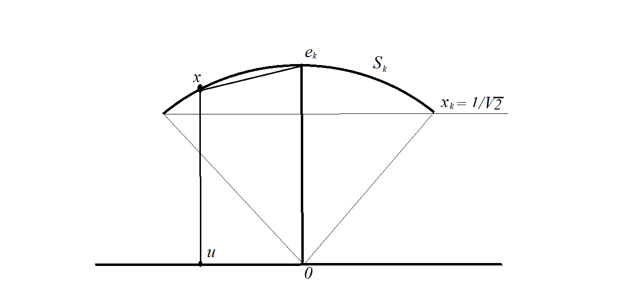
Figure 1. Relationship between $\|u\|$ and $\|x-e_{k}\|$.

Now we should estimate the norm of the vector $h^{\prime}(u)$ through the norm $\|P_{T_{x}}f^{\prime}(x)\|$ from above. Define the function $\phi(u)=[u,\sqrt{1-\|u\|^{2}}]$, ”restoring” a vector $x\in S_{k}$ by its part $u$.

Firstly, $h(u)=f(\phi(u))$, thus $h^{\prime}(u)=f^{\prime}(x)\phi^{\prime}(u)$, here $\phi^{\prime}$ is the Jacobi matrix for the function $\phi(\cdot)$:

$$\phi^{\prime}(u)=\begin{bmatrix}1&0&\cdots&0&0\\ 0&1&\cdots&0&0\\ \vdots&\vdots&\ddots&\vdots&\vdots\\ 0&0&\cdots&1&0\\ 0&0&\cdots&0&1\\ \frac{-u_{1}}{\sqrt{1-\|u\|^{2}}}&\frac{-u_{2}}{\sqrt{1-\|u\|^{2}}}&\cdots&\frac{-u_{n-2}}{\sqrt{1-\|u\|^{2}}}&\frac{-u_{n-1}}{\sqrt{1-\|u\|^{2}}}&\end{bmatrix}$$

$$=\begin{bmatrix}1&0&\cdots&0&0\\ \vdots&\vdots&\ddots&\vdots&\vdots\\ 0&0&\cdots&0&1\\ \frac{-x_{1}}{\sqrt{1-\|u\|^{2}}}&\frac{-x_{2}}{\sqrt{1-\|u\|^{2}}}&\cdots&\frac{-x_{n-1}}{\sqrt{1-\|u\|^{2}}}&\frac{-x_{n}}{\sqrt{1-\|u\|^{2}}}&\end{bmatrix}\in\mathbb{R}^{n\times(n-1)}$$

(there is no column with $x_{k}$ in the last matrix). Let $\ell\in\mathbb{R}^{m}$ be a unit vector. We shall estimate the norm of $\phi^{\prime}(u)$:

$$\|\phi^{\prime}(u)\ell\|^{2}=\sum_{j=1}^{n-1}\ell_{j}^{2}+\Bigg{(}\sum_{\scriptsize\begin{matrix}i=1,n\\ i\neq k\end{matrix}}\frac{x_{i}\ell_{i_{+}}}{\sqrt{1-\|u\|^{2}}}\Bigg{)}^{2}\leq 1+\frac{\|u\|^{2}}{1-\|u\|^{2}}\leq 2.$$

We use the inclusion $x\in S_{k}$ in the last inequality that means $\|u\|\leq 1/\sqrt{2}$ and a technical index

$$i_{+}=\left\{\begin{matrix}i,&\text{ }i<k,\\ i-1,&\text{ }i>k.\end{matrix}\right.$$

Finally we have $\|\phi^{\prime}(u)\ell\|\leq\sqrt{2}$.

Substitute a unit vector $\ell(u)$ with $\|h^{\prime}(u)\|=(h^{\prime}(u),\ell(u))$. Then

$$\|h^{\prime}(u)\|=|(h^{\prime}(u),\ell(u))|=|(\phi^{\prime}(u)^{T}f^{\prime}(\phi(u)),\ell(u))|=|(f^{\prime}(\phi(u)),\phi^{\prime}(u)\ell(u))|$$

$$=\|f^{\prime}(\phi(u))\|\cdot\|\phi^{\prime}(u)\ell(u)\|\cdot\cos\beta\leq\sqrt{2}\|f^{\prime}(x)\|\cdot\cos\beta,$$

here $\beta\leq\pi/2$ is the angle between directions of vectors $f^{\prime}(x)$ and $\phi^{\prime}(u)\ell(u)$. Denote by $\gamma$ the angle between $f^{\prime}(x)$ and the tangent subspace $T_{x}$. We have $\phi^{\prime}(u)\ell(u)\in T_{x}$, hence $\gamma\leq\beta$ and

(26) $$\|h^{\prime}(u)\|\leq\sqrt{2}\|f^{\prime}(x)\|\cos\beta\leq\sqrt{2}\|f^{\prime}(x)\|\cos\gamma=\sqrt{2}\|P_{T_{x}}f^{\prime}(x)\|.$$

By inequalities (24), (25) and (26) we get

$$\frac{\|x-e_{k}\|}{\sqrt{2}}\leq\|u\|\leq\frac{1}{2\mu}\|h^{\prime}(u)\|\leq\frac{1}{\sqrt{2}\mu}\|P_{T_{x}}f^{\prime}(x)\|.$$

So, $\rho(x,\Omega)\leq\frac{1}{\mu}\|P_{T_{x}}f^{\prime}(x)\|$. ∎

5.5. Proof of Theorem 2

In the present section a lower index means the number of the point in a finite set, but not a number of iteration.

Proof.

By Lemma 1 the set of stationary points in nondegenerate problem is finite ($\Omega=\{x_{j}\}_{j=1}^{J}$).

The set $S$ is compact $\mathcal{C}^{2}$-smooth manifold and $f\in\mathcal{C}^{2}$, hence the function

$$S\ni x\to\lambda_{x}=-(g^{\prime}(x)g^{\prime}(x)^{T})^{-1}g^{\prime}(x)f^{\prime}(x)$$

is Lipschitz continuous with some constant $L_{\lambda}$.

From the definition of stationary points $F(x_{j},\lambda_{x_{j}})=0$. Then from differentiability of $F(z)$ by the Taylor formula we have for any $j\in\{1,\dots,J\}$

$$F_{x}(x)\doteq F(x,\lambda_{x})=F(x,\lambda_{x})-F(x_{j},\lambda_{x_{j}})=F^{\prime}(x_{j},\lambda_{x_{j}})\begin{bmatrix}x-x_{j}\\ \lambda_{x}-\lambda_{x_{j}}\end{bmatrix}+o_{j}(\varrho),\ \varrho\to+0,$$

here $\varrho=\sqrt{\|x-x_{j}\|^{2}+\|\lambda_{x}-\lambda_{x_{j}}\|^{2}}\leq\|x-x_{j}\|\sqrt{1+L_{\lambda}^{2}}$.

By the inverse operator theorem condition of non-degeneracy of the problem $\|F^{\prime}(x_{j},\lambda_{x_{j}})^{-1}\|\leq\sigma_{0}$, $j=1,...,J$, is equivalent to the condition

$$\|F^{\prime}(x_{j},\lambda_{x_{j}})h\|\geq\frac{1}{\sigma_{0}}\|h\|,\;\;\forall h\in\mathbb{R}^{n+m},\;j=1,...,J.$$

Choose such a number $\ell>0$ that for all $j=1,...,J$ and $h\in\mathbb{R}^{n+m},\;\|h\|\leq\ell$, the estimate $\|o_{j}(\|h\|)\|\leq\frac{1}{2\sigma_{0}}\|h\|$ is fulfilled.

Fix $x\in S$, $\rho(x,\Omega)\leq\frac{\ell}{\sqrt{1+L_{\lambda}^{2}}}$. Using the Taylor expansion with respect to the nearest point $x_{j}\in\Omega$ at the point $x$ and taking in mind that $\varrho\leq\|x-x_{j}\|\sqrt{1+L_{\lambda}^{2}}\leq\ell$ we have

$$\|F_{x}(x)\|\geq\left\|F^{\prime}(x_{j},\lambda_{x_{j}})\begin{bmatrix}x-x_{j}\\ \lambda_{x}-\lambda_{x_{j}}\end{bmatrix}\,\right\|-\|o_{j}(\varrho)\|\geq\frac{1}{\sigma_{0}}\varrho-\frac{1}{2\sigma_{0}}\varrho=\frac{1}{2\sigma_{0}}\varrho$$

$$\geq\frac{1}{2\sigma_{0}}\|x-x_{j}\|=\frac{1}{2\sigma_{0}}\rho(x,\Omega).$$

Thus the tEB condition holds

(27) $$\|P_{T_{x}}f^{\prime}(x)\|=\|F_{x}(x)\|\geq\mu\rho(x,\Omega),\quad\forall x\in\cup_{j=1}^{J}\mathrm{int}\,B_{r}(x_{j}),$$

where $\mu=1/(2\sigma_{0})$, $r=\frac{\ell}{\sqrt{1+L_{\lambda}^{2}}}$.

The function $F_{x}(x)$ is continuous on the compact set $S_{1}=\left\{x\in S:\rho(x,\Omega)\geq\frac{\ell}{\sqrt{1+L_{\lambda}^{2}}}\right\}$. From $S_{1}\cap\Omega=\emptyset$ we get $\|F_{x}(x)\|>0$ for all $x\in S_{1}$. By the Weierstrass theorem there exists a number $b>0$ such that $\|F_{x}(x)\|\geq b>0$ for all $x\in S_{1}$. Since $\mathrm{diam}\,S=\sup_{x,y\in S}\|x-y\|\geq\rho(x,\Omega)$, then

(28) $$\|F_{x}(x)\|\geq b=\frac{b}{\mathrm{diam}\,S}\mathrm{diam}\,S\geq\frac{b}{\mathrm{diam}\,S}\rho(x,\Omega),\;\;\forall x\in S:\rho(x,\Omega)>\frac{\ell}{\sqrt{1+L_{\lambda}^{2}}}.$$

Combining inequalities (27) and (28), we prove the tEB condition on the set $S$:

$$\|F_{x}(x)\|\geq\min\Big{\{}\frac{1}{2\sigma_{0}},\frac{b}{\mathrm{diam}\,S}\Big{\}}\rho(x,\Omega),\;\;\forall x\in S.$$

∎

5.6. Proof of Lemma 3

The proof is based on the estimate $\|(I+X)^{-1}\|\leq 1/(1-\|X\|)$, $\|X\|<1$.

Proof.

Suppose that a point $x$ is at a distance no more than $r=\beta/(\sigma_{0}L_{1,Fx})$ from some stationary point $x_{*}$, say, the nearest. Denote

$$\Delta F^{\prime}=\Delta F^{\prime}(x)=F^{\prime}(x,\lambda_{x})-F^{\prime}(x_{*},\lambda_{x_{*}}).$$

Fix $\beta\in(0,1)$. We have $\|F^{\prime}(x,\lambda_{x})^{-1}\|=$

$$=\|(F^{\prime}(x_{*},\lambda_{x_{*}})+\Delta F^{\prime})^{-1}\|\leq\|F^{\prime}(x_{*},\lambda_{x_{*}})^{-1}\|\cdot\left\|\left(I+F^{\prime}(x_{*},\lambda_{x_{*}})^{-1}\Delta F^{\prime}\right)^{-1}\right\|\leq$$

$$\leq\frac{\sigma_{0}}{1-\|F^{\prime}(x_{*},\lambda_{x_{*}})^{-1}\Delta F^{\prime}\|}\leq\frac{\sigma_{0}}{1-\|F^{\prime}(x_{*},\lambda_{x_{*}})^{-1}\|\cdot\|\Delta F^{\prime}\|}\leq\frac{\sigma_{0}}{1-\sigma_{0}\|\Delta F^{\prime}\|}.$$

Taking into account the estimate $\|\Delta F^{\prime}\|\leq L_{1,Fx}\|x-x_{*}\|\leq L_{1,Fx}r\leq\frac{\beta}{\sigma_{0}}$ and the last formula we obtain the statement of Lemma. ∎

5.7. Proof of Theorem 3

Recall the expression for constant $C$:

$$C=\min\left\{\frac{\mu\beta}{L_{1,Fx}\sigma_{0}},\;\frac{(1-\beta)^{2}}{4L_{1,F}\sigma_{0}^{2}}\right\}.$$

Proof.

By Corollary 1 the GPA in no more than $N_{1}(C)=\left\lceil\frac{2\Delta f(1+\gamma L_{1})^{2}}{C^{2}\gamma(1-\gamma L_{1})}\right\rceil$ steps will achieve a point $\widehat{x}\in S$, where condition (10) (and (12)) holds. Moreover, some conditions will be met simultaneously.

Firstly, by $\|P_{T_{\widehat{x}}}f^{\prime}(\widehat{x})\|\leq\frac{\mu\beta}{\sigma_{0}L_{1,Fx}}$ and the tEB condition we obtain that the point $\widehat{x}$ is close to some stationary point, i.e. $\rho(\widehat{x},\Omega)\leq\frac{\|P_{T_{x}}f^{\prime}(\widehat{x})\|}{\mu}\leq\frac{\beta}{\sigma_{0}L_{1,Fx}}$. From condition of Theorem $\beta\leq L_{1,Fx}\sigma_{0}d$ it follows that $\rho(\widehat{x},\Omega)<d$ and condition of Lemma 3 is fulfilled. Thus we have the estimate $\|F^{\prime}(\widehat{x},\lambda_{\widehat{x}})^{-1}\|\leq\frac{\sigma_{0}}{1-\beta}$.

Secondly, by virtue of the choice of constant $C$

$$\|F(\widehat{x},\lambda_{\widehat{x}})\|=\|P_{T_{\widehat{x}}}f^{\prime}(\widehat{x})\|\leq\frac{(1-\beta)^{2}}{4L_{1,F}\sigma_{0}^{2}}\leq\frac{1}{4L_{1,F}\|F^{\prime}(\widehat{x},\lambda_{\widehat{x}})^{-1}\|^{2}}$$

and from (15) we get

(29) $$2\|F^{\prime}(\widehat{x},\lambda_{\widehat{x}})^{-1}F(\widehat{x},\lambda_{\widehat{x}})\|\leq 2\frac{\sigma_{0}}{1-\beta}\frac{(1-\beta)^{2}}{4L_{1,F}\sigma_{0}^{2}}=\frac{1-\beta}{2L_{1,F}\sigma_{0}}\leq r.$$

Let $x_{j}\in\Omega$ be a nearest point to the point $\widehat{x}$. From the equalities $d\sqrt{1+L_{\lambda}^{2}}=r$, $\rho(\widehat{x},\Omega)=\|\widehat{x}-x_{j}\|<d$ and Lipschitz condition for $\lambda_{x}$ we have

$$\rho([\widehat{x},\lambda_{\widehat{x}}],\Sigma)\leq\|[\widehat{x},\lambda_{\widehat{x}}]-[x_{j},\lambda_{x_{j}}]\|\leq\rho(\widehat{x},\Omega)\sqrt{1+L^{2}_{\lambda}}\leq r$$

i.e. $F^{\prime}(z)$ is Lipschitz with constant $L_{1,F}$ on the ball $B_{r}([\widehat{x},\lambda_{\widehat{x}}])$.

From the Lipschitz property for $F^{\prime}(z)$ on the ball $B_{r}([\widehat{x},\lambda_{\widehat{x}}])$ and formula (29) by Proposition 2 the sequence $\widehat{x}_{k}$ converges to a stationary point $x_{*}\in\Omega$ with rate

$$\|\widehat{x}_{k}-x_{*}\|\leq 2^{1-k}\|F^{\prime}(\widehat{x},\lambda_{\widehat{x}})^{-1}\|C\leq 2^{1-k}\frac{C\sigma_{0}}{1-\beta}.$$

For an arbitrary $\varepsilon>0$ the number of steps of the modified NM for the accuracy $\rho(\widehat{x}_{k},\Omega)\leq\varepsilon$ can be estimated as follows

$$N_{2}(\varepsilon)=\Bigg{\lceil}\log_{2}\Big{(}\frac{C\sigma_{0}}{\varepsilon(1-\beta)}\Big{)}\Bigg{\rceil}+1.$$

∎

References

- [1] Yu. A. Chernyaev, An extension of the gradient projection method and Newton’s method to extremum problems constrained by a smooth surface, Computational Mathematics and Mathematical Physics, 2015, 55:9, p. 1451-1460.
- [2] M. Balashov, B. Polyak, A. Tremba, Gradient projection and conditional gradient methods for constrained nonconvex minimization. (2019) arXiv:1906.11580
- [3] J.-P. Vial, Strong and Weak Convexity of Sets and Functions. Mathematics of Operations Research, 1983, 8:2, pp. 231–259.
- [4] F. H. Clarke, R. J. Stern, P. R. Wolenski, Proximal smoothness and lower– property, J. Convex Anal., 2:1-2 (1995), 117–144.
- [5] H. Karimi, J. Nutini, M. Schmidt, Linear convergence of gradient and proximal-gradient methods under the Polyak-Lojasiewicz condition. In: Frasconi P., Landwehr N., Manco G., Vreeken J. (eds) Machine Learning and Knowledge Discovery in Databases. Lecture Notes in Computer Science, vol 9851. Springer, 2016.
- [6] D. Drusvyatskiy, A.S. Lewis, Error bounds, quadratic growth, and linear convergence of proximal methods, (2016), arXiv:1602.06661
- [7] B. Gao, X. Liu, X. Chen, Ya. Yuan, On the Lojasiewicz exponent of the quadratic sphere constrained optimization problem, (2016), arXiv:1611.08781v2
- [8] H. Liu, W. Wu, A. M.-Ch. So, Quadratic Optimization with Orthogonality Constraints: Explicit Lojasiewicz Exponent and Linear Convergence of Line-Search Methods. (2015), arXiv:1510.01025
- [9] P.-A. Absil, R. Mahony, R. Sepulchre, Optimization Algorithms on Matrix Manifolds, Princeton University Press, Princeton and Oxford, 2008.
- [10] J.-P. Aubin, I. Ekeland, Applied Nonlinear Analysis. Wiley, 1984.
- [11] D.P. Bertsekas, Nonlinear programming, Massachusetts, Athena Scientific, 2nd ed., 1999. 777p.
- [12] B. T. Polyak, Introduction to optimization, NY, Translation series of mathematics and engineering, 1987.
- [13] R. A. Poliquin, R. T. Rockafellar, L. Thibault, Local Differentiability of Distance Functions. Transactions of the American Mathematical Society, 352:11 (Nov., 2000), pp. 5231–5249.
- [14] M. Bounkhel and L. Thibault, On various notions of regularity of sets in nonsmooth analysis, Nonlin. Anal. 48 (2002), 223-246.
- [15] M. V. Balashov Nonconvex optimization. — In book: Control theory (additional chapters): Tutorial / Ed. D. A. Novikov. M.: Leland, 2019. 552 p. In russian.
- [16] Kolmogorov A. N., Fomin S. V. Elements of the function theory and functional analysis. – 7th ed. – M.: Fizmatlit, 2004. In russian.
- [17] Yu. Nesterov, Lectures on Convex Optimization, Springer, 2018.
- [18] P.-A. Absil, J. Malick, Projection-like retractions on matrix manifolds. SIAM Journal on Optimization, Society for Industrial and Applied Mathematics, 2012, 22:1, pp. 135-158.
- [19] M. V. Balashov. The gradient projection algorithm for a proximally smooth set and a function with Lipschitz continuous gradient. Sbornik: Mathematics, N 6, 2020. In press.