Limits on Kaluza-Klein dark matter annihilation in the Sun from recent IceCube results

Abstract

We interpret recent IceCube results on searches for dark matter accumulated in the sun in terms of the lightest Kaluza-Klein excitation (assumed here to be the Kaluza-Klein photon, $B^{1}$), obtaining improved limits on the annihilation rate in the Sun, the resulting neutrino flux at the Earth and on the $B^{1}$-proton cross-sections, for $B^{1}$ masses in the range 30–3000 GeV. These results improve previous results from IceCube in its 22-string configuration by up to an order of magnitude, depending on mass, but also extend the results to $B^{1}$ masses as low as 30 GeV.

1 Introduction

There are many astrophysical and cosmological observations that point to the existence of a dark matter component as a key constituent of the Universe. Constraints on the amount of baryons in the Universe from CMB measurements, from measurements of the abundance of primordial light elements and from searches for dark objects using microlensing have practically ruled out the possibility that dark matter consists of known Standard Model particles Garrett:2010hd . In the most popular picture, dark matter is composed by non-relativistic Weakly Interacting Massive Particles (WIMPs) of yet unknown nature Bertone:2004pz . Among the many theories beyond the Standard Model of particle physics that predict new particles that could be viable dark matter candidates, Kaluza-Klein type models Kaluza:1921tu ; Klein:1926tv with universal extra dimensions (UED) provide a WIMP in the Kaluza-Klein photon ($B^{1}$), the first excitation of the scalar gauge boson in the theory Cheng:2002ej ; Hooper:2002gs ; Servant:2002aq ; Hooper:2007qk ; Blennow:2009ag ; Flacke:2017xsv . Usually denoted as the lightest Kaluza-Klein particle (LKP), it can have a mass in the range from a few hundred GeV (limit from rare decay processes Freitas:2008vh ; Haisch:2007vb ) to a few TeV (to avoid overclosing the Universe), the mass being proportional to 1/R, where R is the size of the extra dimension.

LKPs in the galactic halo will suffer the same fate as any other WIMP. Assuming a non-zero $B^{1}$–proton scattering cross section, $B^{1}$’s in the galactic halo with Sun-crossing orbits can loose energy through interaction with the matter in the Sun and eventually sink into its core, where they would accumulate and annihilate into Standard Model particles Spergel:1984re ; Press:1985ug ; Gaisser:1986ha , which in turn can lead to a detectable neutrino flux. Neutrino telescopes like AMANDA, IceCube, ANTARES and Baikal have searched for signatures of dark matter in this way, mainly focusing on the SUSY neutralino as WIMP candidate IceCube:2011aj ; Aartsen:2016zhm ; Adrian-Martinez:2016gti ; Avrorin:2014swy . Additionally, both IceCube and ANTARES have set limits to the spin-dependent LKP-proton cross section Abbasi:2009vg ; Zornoza:2013ema . The IceCube limits are based on the event selection and analysis searching for WIMP dark matter performed in Abbasi:2009uz .

In this letter we use the latest dark matter searches from the Sun by IceCube Aartsen:2016zhm to improve the limits on the Kaluza-Klein photon cross section with protons. Given the increase in detector size (86 strings versus 22 in the previous IceCube analysis) and lifetime (104 d versus 532 d) the results presented in this letter improve those in Abbasi:2009vg by up to an order of magnitude. Additionally, the presence of the low-energy subdetector DeepCore allows to lower the explored LKP mass down to 30 GeV, compared to 250 GeV, the lowest mass studied in Abbasi:2009vg .

2 LKP signatures from the Sun

Table 1: Table with the branching ratios of the main annihilation channels of $B^{1}B^{1}\rightarrow X\overline{X}$ in terms of two values of the quark splitting mass. The last channel corresponds to a Higgs-anti-Higgs pair. Source: Hooper:2002gs

Channel	$\Delta m=0$	$\Delta m=0.14$
$\nu_{e}\overline{\nu}_{e},\nu_{\mu}\overline{\nu}_{\mu},\nu_{\tau}\overline{\nu}_{\tau}$	0.012	0.014
$e^{+}e^{-},\mu^{+}\mu^{-},\tau^{+}\tau^{-}$	0.20	0.23
$u\overline{u},c\overline{c},t\overline{t}$	0.11	0.077
$d\overline{d},s\overline{s},b\overline{b}$	0.007	0.005
$\phi\overline{\phi}$	0.023	0.027

Table 1 shows the theoretical branching ratios of the $B^{1}$ self-annihilation processes in terms of the quark splitting mass:

$$\Delta m=\frac{m_{q^{1}}-m_{B^{1}}}{m_{B^{1}}},$$ (1)

where $m_{q^{1}}$ is the first fermion excitation in the Kaluza-Klein theory within Universal Extra Dimensions Hooper:2002gs . The mass at which the LKP can be a good dark matter candidate depends on this splitting, which drives the co-annihilation with the higher KK modes which, in turn, determines the relic abundance Belanger:2010yx . Among the final annihilation products, only the weakly interacting neutrinos are able to escape from the Sun and be detected in neutrino observatories on Earth. Neutrinos resulting from these annihilations are also expected to be easily distinguishable from thermonuclear reaction products because the value of $B^{1}$ mass needed for it to be a good dark matter candidate ($m_{B^{1}}>{\cal{O}}100$ GeV).

Assuming that the capture and annihilation rates of $B^{1}$ particles in the Sun, $\Gamma_{C}$ and $\Gamma_{A}$, have reached an equilibrium Hooper:2002gs ; Wikstrom:2009kw , the relationship between them can be written as $\Gamma_{A}=\frac{1}{2}\Gamma_{C}$, where the one half factor comes from the fact that one annihilation requires two captured $B^{1}$. This means that, assuming a particular velocity distribution for dark matter in the solar neighborhood and a solar structure model, the $B^{1}$–proton scattering cross section, which drives the capture, is proportional to the annihilation rate,

$$\sigma^{i}=\lambda^{i}\left(m_{B^{1}}\right)\Gamma_{A}$$ (2)

where the proportionality constant $\lambda^{i}\left(m_{B^{1}}\right)$ depends on the mass of the $B^{1}$, and the superscript $i$ can take the values SD (for spin-dependent cross section) or SI (for spin-independent cross section). The neutrinos produced in the core of the Sun have to be numerically propagated to a detector on Earth to predict the detectable neutrino flux per unit area and time in the detector, $\Phi_{\nu}$, which is proportional to the annihilation rate, $\Phi_{\nu}=\eta\left(m_{B^{1}}\right)\Gamma_{A}$. Such neutrino propagation must also take into account the solar composition, neutrino interaction processes with matter (such as absorption, re-emission, decays of secondary particles into neutrinos, etc.) and neutrino oscillations.

We simulated one million annihilation events at the core of the Sun and we propagated the neutrinos to a detector in the ice at latitude $90^{\circ}$ S during the austral winter using WimpSim Edsjo:XXX , for different assumed values of $m_{B^{1}}$. The simulations themselves do not include any information on the capture conditions or $\Gamma_{A}$, but they do require a solar structure model as an input for the propagation of neutrinos, in this case the one from Serenelli:2009yc . Figure 1 shows the energy distribution of the muon (plus anti-muon) neutrino fluxes at the Earth per unit area $A$ and per annihilation in the Sun, as a function of reduced energy $z=E_{\nu}/m_{B^{1}}$,

$$\frac{d\Psi_{\nu}}{dz}=\frac{dN_{\nu}}{dAdN_{A}dz}$$ (3)

for some values of $m_{B^{1}}$.

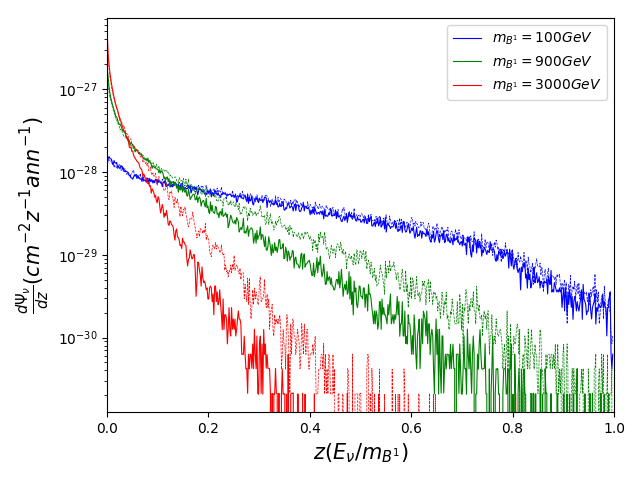
Figure 1: Predicted energy spectra of muon neutrinos (solid lines) and anti-muon neutrinos (dashed lines) at the detector from ${B^{1}}$ annihilations, for three different values of $m_{B^{1}}$. An extra peak at the end of the spectra produced by neutrinos that escape the Sun without interacting has been omitted from the plot for the sake of legibility, but it is considered in the calculations. Note the normalization in relative energy units.

As expected, heavier $B^{1}$ particles produce steeper profiles in energy because of absorption of high-energy neutrinos on their way out of the Sun. The convolution of those spectra with the effective area of the detector gives a prediction of the number of events $\mu_{s}$ per number of annihilations $N_{A}$, expected at the detector

$$\frac{d\mu_{s}}{dN_{A}}=\int_{0}^{1}\frac{d\Psi_{\nu}}{dz}A_{eff}\left(z\right)dz$$ (4)

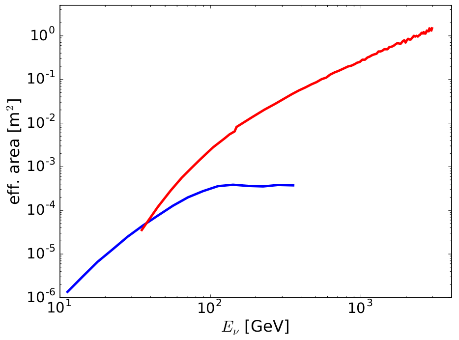
Figure 2: The combined muon and anti-muon neutrino effective area for both the DeepCore (blue) and main IceCube array (red) for horizontally arriving neutrinos as a function of the neutrino energy. Uncertainties are not shown, but they can be as large as $30\%$. Source: Aartsen:2016zhm

In order to take into account the finite angular resolution of the detector, the direction of each event has been randomly smeared using the median angular resolution of IceCube shown in Figure 3, which has been computed from the median muon neutrino energy at every $m_{B^{1}}$ and the corresponding mean angular separation between the original neutrino and the reconstructed muon trajectories (see Aartsen:2016zhm for the explicit relation). $\Theta$ is used to spread the predicted signal (4) with a 2D Gaussian distribution centered around the Sun on the celestial sphere:

$$\frac{d\mu_{s}}{dN_{A}d\psi}=\frac{d\mu_{s}}{dN_{A}}\frac{C}{\Theta^{2}}e^{-\psi^{2}/2\Theta^{2}}\sin{\psi}$$ (5)

where $\psi$ is the angle from the Sun ($\psi_{\odot}=0$), and $C$ a normalization constant. The expected angular distribution of the signal, for a few ${B^{1}}$ masses as a function of angle with respect to the Sun position is shown in figure 5.

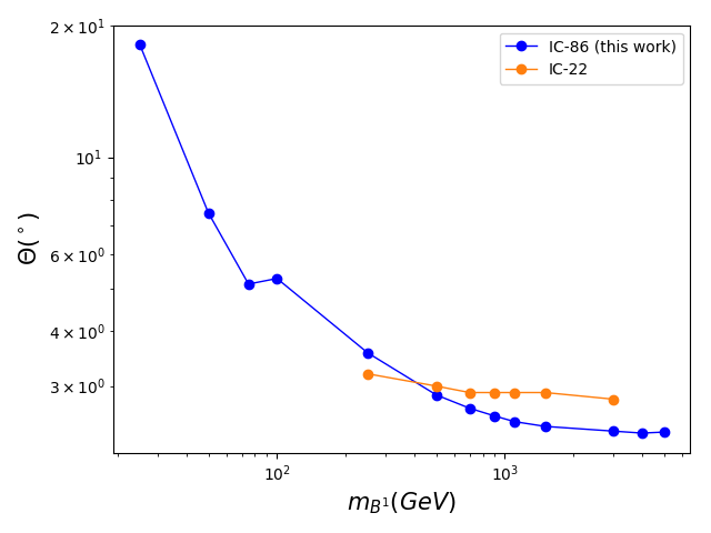
Figure 3: Median angular resolution as a function of $B^{1}$ mass for the 86-string configuration (blue) and the 22-string configuration (orange). The bump at $m_{B^{1}}=100$ GeV in the former is due to the transition from DeepCore resolution to IceCube resolution Aartsen:2016zhm

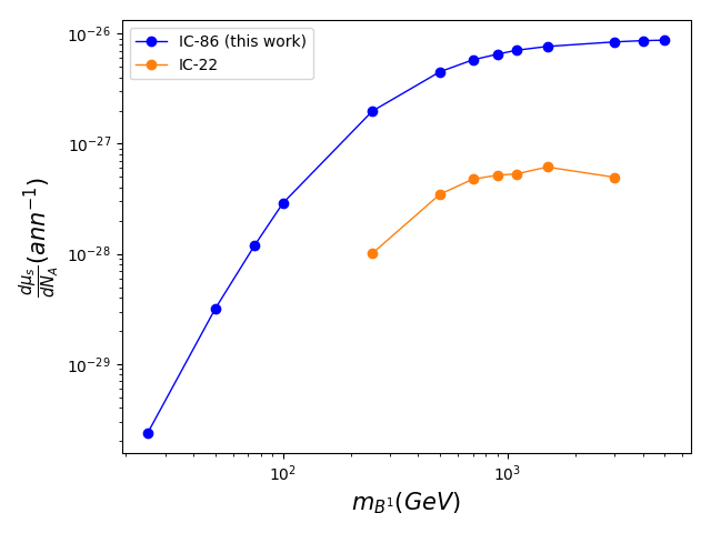
Figure 4: Expected number of events in IceCube per annihilation as a function of $B^{1}$ mass. The blue dots show the result of this work (using equation 4 with the effective area of reference Aartsen:2016zhm ), while the orange dots show, for comparison, the result using the effective area of the 22-string IceCube configuration Abbasi:2009uz , which was the basis for the previous Kaluza-Klein analysis Abbasi:2009vg . Lines are just a linear interpolation between the dots to guide the eye.

3 Data selection

We use the muon-neutrino effective area corresponding to the latest solar dark matter search from IceCube Aartsen:2016zhm , shown in Figure 2. The figure shows the effective areas for IceCube and DeepCore for muon neutrinos as a function of neutrino energy, $E_{\nu}$, for the case of neutrinos arriving near the horizon, since the Sun is always close to the horizon in the South Pole. For this analysis, both curves are summed and the entire detector is treated as one single array. Only muon events are considered here since the long muon tracks allow pointing back to the Sun. Muon in what follows refer to both muons and anti-muons since IceCube can not distinguish between particles and antiparticles.

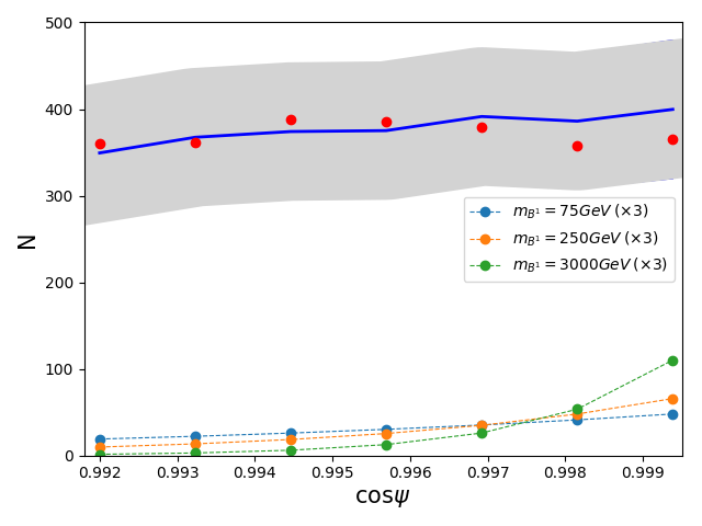
Figure 5: Expected background (dark blue line) within the range of maximum systematic uncertainties (shaded area), the actual number of detected events at every angular bin (red dots) and the expected signal (multiplied by three for visualization) for some values of $m_{B^{1}}$ (light blue, orange and green), as a function of angle with respect to the Sun. Data from Aartsen:2016zhm .

The predicted signal (equation 4) can be compared with the actual observed signal rate to compute $\Gamma_{A}$:

$$\frac{d\mu_{s}}{dt}=\frac{dN_{A}}{dt}\frac{d\mu_{s}}{dN_{A}}=\Gamma_{A}\frac{d\mu_{s}}{dN_{A}}$$ (6)

and $\Gamma_{A}$ is used to calculate the $B^{1}$–proton scattering cross sections through equation (2). The conversion factors $\lambda^{i}\left(m_{B^{1}}\right)$ are obtained with the DarkSUSY software Bringmann:2018lay , and include the information on the solar structure and the dark matter velocity distribution in the solar neighborhood Wikstrom:2009kw . Figure 4 shows the expected number of events at the detector per annihilation as a function of $B^{1}$ mass calculated with equation (4)

We use the data from Figure 6 in Aartsen:2016zhm , which we present here combined for DeepCore and IceCube in Figure 5, in order to extract limits on the spin-dependent $B^{1}$-proton cross section as a function of $B^{1}$ mass. The data set was obtained during 532 days of exposure between May 2001 and May 2014. As thoroughly explained in Aartsen:2016zhm , several filters were applied to the data sample in order to minimize the presence of background. Data was only taken into account if measured during austral winters, when the Sun is below the horizon, in order to avoid overlap with atmospheric muons originating from cosmic-ray induced showers in the atmosphere above the detector. For this reason, only muons with upward trajectories were selected. Still, atmospheric muon neutrinos created at any declination can cross the Earth without interacting and reach the detector from below, being an irreducible background. Boosted Decision Trees were used to maximize signal separation and reduce background.

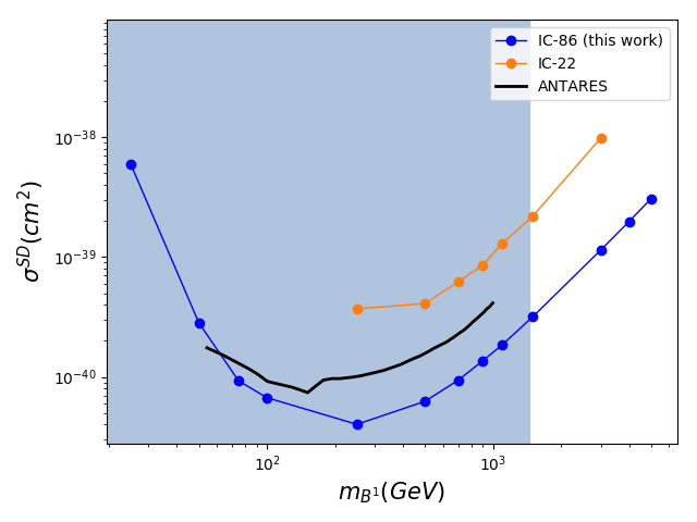
Figure 6: 90% confidence level upper limit on the spin-dependent $B^{1}$–proton scattering cross section as a function of $B^{1}$ mass. Blue: this work. Orange: previous IceCube limit on LKP cross section from Abbasi:2009vg . Black line: limits from ANTARES Zornoza:2013ema . The shaded area represents the disfavoured region (at 95% confidence level) on the mass of the LKP from the LHC Deutschmann:2017bth .

4 Results

Figure 5 shows that no statistically significant deviation from the expected background was detected in the IceCube solar analysis, so a 90% confidence level limit on the $B^{1}$-proton cross section can be extracted from the data by setting a limit to $\Gamma_{A}$. The amount of expected signal events per unit of time can be estimated as

$$\frac{d\mu_{s}}{dt}\simeq\frac{\mu_{s}}{\tau}$$ (7)

where $\tau$ is the total exposure time, 532 days in our case. We proceed with a “counting experiment”, comparing the number of background events to the number of observed events extracted from Figure 5, and construct Poisson confidence intervals for the signal strength $\mu_{s}$, calculated with the Neyman method using the algorithm developed in Conrad:2002kn , including the detector systematic uncertainties from Aartsen:2016zhm . A limit on $\mu_{s}$ is easily translated to a limit on $\Gamma_{A}$ through equation (6) and further to limits on $\sigma^{SI}$ and $\sigma^{SD}$ through equation (2). Table 2 shows the results for a series of $B^{1}$ masses. Limits at 90% confidence level on the signal strength ($\mu_{s}$), the annihilation rate in the Sun ($\Gamma_{A}$), the muon flux at the detector above 1 GeV ($\Phi_{\mu}$) and the spin-independent and spin-dependent cross sections ($\sigma^{SI}$ and $\sigma^{SD}$) are shown, along with the median angular resolution ($\Delta\theta_{\nu}$) and mean muon energy at the detector ($\left<E_{\mu}\right>$) for each signal model.

Table 2: 90% confidence level upper limits on the signal, the annihilation rate in the Sun, the muon flux at the detector above 1 GeV and the spin independent and spin dependent $B^{1}$-proton cross sections for several values of the $B^{1}$ mass. The last two columns show the median angular resolution and the muon mean energy at the detector.

$m_{B^{1}}$	$\mu_{s}$	$\Gamma_{A}$	$\Phi_{\mu}$	$\sigma^{SI}$	$\sigma^{SD}$	$\Delta\theta_{\nu}$	$\left<E_{\mu}\right>$
(GeV)		(ann$\cdot$ s-1)	(km-2y-2)	(cm2)	(cm2)	(∘)	(GeV)
25	907.6	$8.3\cdot 10^{24}$	$2.0\cdot 10^{4}$	$5.1\cdot 10^{-41}$	$6.0\cdot 10^{-39}$	$\pm 18.1$	$6.8$
50	186.7	$1.3\cdot 10^{23}$	$1.1\cdot 10^{3}$	$1.4\cdot 10^{-42}$	$2.8\cdot 10^{-40}$	$\pm 7.5$	$13.3$
75	111.8	$2.0\cdot 10^{22}$	$3.5\cdot 10^{2}$	$3.4\cdot 10^{-43}$	$9.3\cdot 10^{-41}$	$\pm 5.1$	$19.3$
100	114.0	$8.6\cdot 10^{21}$	$2.5\cdot 10^{2}$	$2.0\cdot 10^{-43}$	$6.7\cdot 10^{-41}$	$\pm 5.3$	$25.8$
250	80.5	$8.9\cdot 10^{20}$	$98$	$7.1\cdot 10^{-44}$	$4.03\cdot 10^{-41}$	$\pm 3.6$	$54.7$
500	73.1	$3.5\cdot 10^{20}$	$76$	$8.3\cdot 10^{-44}$	$6.3\cdot 10^{-41}$	$\pm 2.9$	$88.0$
700	72.16	$2.7\cdot 10^{20}$	$73$	$1.1\cdot 10^{-43}$	$9.4\cdot 10^{-41}$	$\pm 2.7$	$107.6$
900	71.77	$2.4\cdot 10^{20}$	$71$	$1.6\cdot 10^{-43}$	$1.4\cdot 10^{-40}$	$\pm 2.6$	$117.1$
1100	71.5	$2.2\cdot 10^{20}$	$71$	$2.1\cdot 10^{-43}$	$1.9\cdot 10^{-40}$	$\pm 2.5$	$126.9$
1500	71.4	$2.0\cdot 10^{20}$	$71$	$3.4\cdot 10^{-43}$	$3.2\cdot 10^{-40}$	$\pm 2.4$	$135.1$
3000	71.3	$1.8\cdot 10^{20}$	$70$	$1.2\cdot 10^{-42}$	$1.1\cdot 10^{-39}$	$\pm 2.4$	$148.3$
4000	71.2	$1.8\cdot 10^{20}$	$70$	$2.0\cdot 10^{-42}$	$2.0\cdot 10^{-39}$	$\pm 2.3$	$150.3$
5000	71.2	$1.8\cdot 10^{20}$	$71$	$3.1\cdot 10^{-42}$	$3.1\cdot 10^{-39}$	$\pm 2.4$	$151.5$

Figure 6 shows $\sigma^{SD}$ versus $B^{1}$ mass for the current analysis (blue dots) and the previously published analysis by IceCube in the 22-string configuration (orange dots), where it can be seen that the constraints have been improved by up to one order of magnitude. The figure also shows the results from the ANTARES collaboration Zornoza:2013ema (black curve). The shaded area shows the disfavoured mass region for the first Kaluza-Klein excitation obtained from searches for UED at the LHC Deutschmann:2017bth , where a limit on 1/R (GeV) is obtained by combining several searches for events with large missing transverse momentum or monojets by ATLAS and CMS at 8 TeV and 13 TeV center of mass energies. Collider searches provide a complementary approach to indirect searches for dark matter in the form of Kaluza-Klein modes with neutrino telescopes, being competitive in different regions of the LKP mass range. Additional constraints from cosmology (that the $B^{1}$ must have a relic density compatible with the estimated dark matter density from CMB measurements) require the mass of the $B^{1}$ to be below $\sim$1.6 TeV Blennow:2009ag ; Belanger:2010yx ; Arrenberg:2008np . Thus, taken all results together, the allowed parameter space for the $B^{1}$ to constitute the only component of dark matter in the Universe is currently quite restricted, but non-minimal UED models, not probed here, can still provide viable dark matter candidates Flacke:2017xsv .

From the experimental point of view, a few simplifying assumptions have been made to obtain the presented results. Uncertainties on the solar structure model and dark matter velocity distribution have been ignored, and binned data (from Figure 5) have been used instead of a continuous sample of individual events, which limits the statistical power of the analysis. Even with these approximations, the IceCube limit presented in this letter considerably improves over those published in Abbasi:2009vg and Zornoza:2013ema .

References

- (1) K. Garrett and G. Duda, “Dark Matter: A Primer,” Adv. Astron. 2011, 968283 (2011)
- (2) G. Bertone, D. Hooper and J. Silk, “Particle dark matter: Evidence, candidates and constraints”, Phys. Rept. 405, 279 (2005)
-
(3)
T. Kaluza, “Zum Unittatsproblem der Physik”,
Sitzungsber. Preuss. Akad. Wiss. Berlin (Math. Phys. ) 1921, 966 (1921).
Also Int. J. Mod. Phys. D 27, no. 14, 1870001 (2018) - (4) O. Klein, “Quantum Theory and Five-Dimensional Theory of Relativity”, Z. Phys. 37, 895 (1926)
- (5) H. C. Cheng, J. L. Feng and K. T. Matchev, “Kaluza-Klein dark matter”,’ Phys. Rev. Lett. 89, 211301 (2002).
- (6) D. Hooper and G. D. Kribs, “Probing Kaluza-Klein dark matter with neutrino telescopes”, Phys. Rev. D 67, 055003 (2003)
- (7) G. Servant and T. M. P. Tait, “Is the lightest Kaluza-Klein particle a viable dark matter candidate?”, Nucl. Phys. B 650, 391 (2003)
- (8) D. Hooper and S. Profumo, “Dark matter and collider phenomenology of universal extra dimensions”, Phys. Rept. 453, 29 (2007)
- (9) M. Blennow, H. Melbeus and T. Ohlsson, “Neutrinos from Kaluza-Klein dark matter in the Sun,” JCAP 1001, 018 (2010)
- (10) T. Flacke, D. W. Kang, K. Kong, G. Mohlabeng and S. C. Park, “Electroweak Kaluza-Klein Dark Matter”, JHEP 1704 041 (2017).
- (11) A. Freitas and U. Haisch, “Anti-B X(s) gamma in two universal extra dimensions”, Phys. Rev. D 77, 093008 (2008)
- (12) U. Haisch and A. Weiler, “Bound on minimal universal extra dimensions from anti-B X(s)gamma,” Phys. Rev. D 76, 034014 (2007)
- (13) D. N. Spergel and W. H. Press, “Effect of hypothetical, weakly interacting, massive particles on energy transport in the solar interior,” Astrophys. J. 294, 663 (1985)
- (14) W. H. Press and D. N. Spergel, “Capture by the sun of a galactic population of weakly interacting massive particles,”, Astrophys. J. 296, 679, (1985)
- (15) T. K. Gaisser, G. Steigman and S. Tilav, “Limits on Cold Dark Matter Candidates from Deep Underground Detectors,” Phys. Rev. D 34 (1986) 2206.
- (16) R. Abbasi et al.,“Multi-year search for dark matter annihilations in the Sun with the AMANDA-II and IceCube detectors,” Phys. Rev. D 85,042002 (2012)
- (17) M. G. Aartsen et al., “Search for annihilating dark matter in the Sun with 3 years of IceCube data,” Eur. Phys. J. C 77 no.3, 146, (2017) Erratum: [Eur. Phys. J. C 79 no.3, 214, (2019)]
- (18) S. Adrian-Martinez et al., “Limits on Dark Matter Annihilation in the Sun using the ANTARES Neutrino Telescope,” Phys. Lett. B 759, 69 (2016)
- (19) A. D. Avrorin et al., “Search for neutrino emission from relic dark matter in the Sun with the Baikal NT200 detector,” Astropart. Phys. 62, 12 (2015)
- (20) R. Abbasi et al., “Limits on a muon flux from Kaluza-Klein dark matter annihilations in the Sun from the IceCube 22-string detector,” Phys. Rev. D 81, 057101 (2010)
- (21) J. D. Zornoza, “Search for Dark Matter in the Sun with the ANTARES Neutrino Telescope in the CMSSM and mUED frameworks,” Nucl. Instrum. Meth. A 725, 76 (2013)
- (22) R. Abbasi et al., “Limits on a muon flux from neutralino annihilations in the Sun with the IceCube 22-string detector,” Phys. Rev. Lett. 102, 201302, (2009)
- (23) G. Belanger, M. Kakizaki and A. Pukhov, “Dark matter in UED: The Role of the second KK level,” JCAP 1102, 009 (2011)
- (24) G. Wikström and J. Edsjö, “Limits on the WIMP-nucleon scattering cross-section from neutrino telescopes,” JCAP 0904, 009 (2009)
- (25) J. Edsjö, J. Elevant and C. Niblaeus, WimpSim Neutrino Monte Carlo, http://wimpsim.astroparticle.se
- (26) A. Serenelli, S. Basu, J. W. Ferguson and M. Asplund, “New Solar Composition: The Problem With Solar Models Revisited,” Astrophys. J. 705, L123 (2009)
- (27) T. Bringmann, J. Edsjö, P. Gondolo, P. Ullio and L. Bergström, “DarkSUSY 6: An Advanced Tool to Compute Dark Matter Properties Numerically,” JCAP 1807, 033, (2018). Also http://www.darksusy.org
- (28) J. Conrad, O. Botner, A. Hallgren and C. Pérez de los Heros, “Including systematic uncertainties in confidence interval construction for Poisson statistics,” Phys. Rev. D 67, 012002 (2003)
- (29) N. Deutschmann, T. Flacke and J. S. Kim, “Current LHC Constraints on Minimal Universal Extra Dimensions,” Phys. Lett. B 771, 515 (2017)
- (30) J. Beuria, A. Datta, D. Debnath and K. T. Matchev, “LHC Collider Phenomenology of Minimal Universal Extra Dimensions,” Comput. Phys. Commun. 226, 187 (2018)
- (31) S. Arrenberg, L. Baudis, K. Kong, K. T. Matchev and J. Yoo, “Kaluza-Klein Dark Matter: Direct Detection vis-a-vis LHC,” PoS IDM 2008, 059 (2008)