Expansion for the critical point of site percolation:
the first three terms

Abstract

We expand the critical point for site percolation on the $d$-dimensional hypercubic lattice in terms of inverse powers of $2d$, and we obtain the first three terms rigorously. This is achieved using the lace expansion.

Mathematics Subject Classification (2010). 60K35, 82B43.

Keywords and phrases. Site percolation, critical threshold, asymptotic series, lace expansion

1 Introduction

We study site percolation on the hypercubic lattice $\mathbb{Z}^{d}$. To this end, we fix a parameter $p\in[0,1]$ and create a random subgraph of $\mathbb{Z}^{d}$ as follows. Each site (or vertex) $x\in\mathbb{Z}^{d}$, independently of all other sites, is declared occupied with probability $p$ (and vacant otherwise). A bond (edge) between two nearest-neighbor sites in $\mathbb{Z}^{d}$ is an edge of the random subgraph if and only if the two sites are occupied. Denote by $\theta(p)$ the probability that there is a path starting at the origin $\mathbf{0}\in\mathbb{Z}^{d}$ and diverging to infinity that consists only of occupied vertices. This allows us to define the critical point as

$$p_{c}:=\inf\big{\{}p\in[0,1]:\theta(p)>0\big{\}}.$$ (1.1)

It is standard that $0<p_{c}<1$ in all dimensions $d\geq 2$. In general, it is not possible to write down an explicit value for $p_{c}=p_{c}(d)$ (see Table 1 for numerical values), a notable exception is site percolation on the two-dimensional triangular lattice (when $p_{c}=1/2$). However, it is possible to derive an asymptotic expansion for $p_{c}(d)$ when $d\to\infty$. Indeed, it is known in the physics literature that

$$p_{c}=\sigma^{-1}+\frac{3}{2}\sigma^{-2}+\frac{15}{4}\sigma^{-3}+\frac{83}{4}\sigma^{-4}+\frac{6577}{48}\sigma^{-5}+\frac{119077}{96}\sigma^{-6}+\cdots\quad\text{for $\sigma={2d-1}\to\infty$.}$$ (1.2)

The first four terms were found by Gaunt, Ruskin, and Sykes in 1976 [5] through exact enumeration, the last two terms have been obtained by Mertens and Moore [16] by exploiting involved numerical methods. When writing this in powers of $\frac{1}{2d}$, (1.2) becomes

$$p_{c}(d)=(2d)^{-1}+\frac{5}{2}(2d)^{-2}+\frac{31}{4}(2d)^{-3}+\frac{75}{2}(2d)^{-4}+\frac{11977}{48}(2d)^{-5}+\frac{209183}{96}(2d)^{-6}+\cdots.$$ (1.3)

In this paper, we extend the previously known first term by establishing the second and third term, including a rigorous bound on the error term.

Theorem 1.1 (Expansion of $p_{c}$ in terms of $(2d)^{-1}$).

As $d\to\infty$,

$$p_{c}(d)=(2d)^{-1}+\frac{5}{2}(2d)^{-2}+\frac{31}{4}(2d)^{-3}+\mathcal{O}\left((2d)^{-4}\right).$$

The key technical tool for our approach is the lace expansion for site percolation. It was established in a recent paper [13], which itself draws its inspiration from Hara and Slade’s seminal paper [11]. The lace expansion provides an expression for $p_{c}$ in terms of lace-expansion coefficients, which are defined in Definition 2.5. Moreover, it provides good control over these coefficients, and the results of [13] identify already the leading order term in (1.3).

Comparison with bond percolation.

It is most instructive to compare the critical thresholds for site and bond percolation. While the critical behaviour of bond- and site percolation is comparable, the actual values of the critical thresholds differ, as illustrated by the following table:

dim	2	3	4	5	6	7	8	9	10	11	12
$p_{c}^{\text{site}}$	0.5927	0.3116	0.1969	0.1408	0.1090	0.0890	0.0752	0.0652	0.0576	0.0516	0.0467
$p_{c}^{\text{bond}}$	$0.5^{\ast}$	0.2488	0.1601	0.1182	0.0942	0.0786	0.0677	0.0595	0.0531	0.0479	0.0437

Table 1: Critical values for percolation on $\mathbb{Z}^{d}$, rounded to multiples of $10^{-4}$. The only rigorously obtained value is for bond percolation in dimension 2 (marked with ^∗). All other values are obtained through numerical simulation; the values for $d\geq 4$ are reported from Grassberger [8] and Mertens and Moore [16].

Grimmett and Stacey [10] prove that $p_{c}^{\text{site}}>p_{c}^{\text{bond}}$ on $\mathbb{Z}^{d}$ for all dimensions $d\geq 2$. This difference must be reflected in the asymptotic expansion for $p_{c}$. Indeed, Hara and Slade [12] and van der Hofstad and Slade [15] rigorously obtain a series expansion for bond percolation as

$$p_{c}^{\text{bond}}(d)=(2d)^{-1}+(2d)^{-2}+\frac{7}{2}(2d)^{-3}+\mathcal{O}\left((2d)^{-4}\right),$$ (1.4)

which indeed differs from the expansion of $p_{c}^{\text{site}}$ in Theorem 1.1. Again, more precise estimates are known by non-rigorous methods [4, 16]:

$$p_{c}^{\text{bond}}=\sigma^{-1}+\frac{5}{2}\sigma^{-3}+\frac{15}{2}\sigma^{-4}+57\sigma^{-5}+\frac{4855}{12}\sigma^{-6}+\cdots$$ (1.5)

for $\sigma={2d-1}$, which is equivalent to

$$p_{c}^{\text{bond}}(d)=(2d)^{-1}+(2d)^{-2}+\frac{7}{2}(2d)^{-3}+16(2d)^{-4}+103(2d)^{-5}+\frac{9487}{12}(2d)^{-6}+\cdots.$$

We remark that (1.4) was proved in [15] also for the $d$-dimensional cube. More recently, an asymptotic expansion was also proven for the Hamming graph [3].

Borel summability of the coefficients.

Theorem 1.1 establishes an expansion to the third order, but it is plausible that even an expansion to all orders for site percolation exist: writing $s=\frac{1}{2d}$ and $\bar{p}_{c}(s)=p_{c}(d)$, this means that there is a real sequence $(\alpha_{n})_{n\in\mathbb{N}}$ such that for any $M\in\mathbb{N}$,

$$\bar{p}_{c}(s)=\sum_{n=1}^{M-1}\alpha_{n}\,s^{n}+\mathcal{O}(s^{M}).$$ (1.6)

The corresponding statement for bond percolation was proved by Hofstad and Slade [14]. However, it is expected that the radius of convergence of the series $\sum\alpha_{n}s^{n}$ is zero (even though rigorous evidence is lacking), and this non-convergence is valid in greater generality for series expansions of critical thresholds of various statistical mechanical models. The reason is that the sequence of absolute values $|\alpha_{1}|,|\alpha_{2}|,|\alpha_{3}|,\dots$ grows very rapidly (with sign changes for higher $n$), and that therefore it is not possible to compute $\bar{p}_{c}(s)$ from the sequence $(\alpha_{n})$.

Instead, we believe that the coefficients $(\alpha_{n})$ are Borel summable: suppose $\bar{p}_{c}(s)$ has an analytic extension to the complex disk $D=\{z\in\mathbb{C}\colon{\rm Re}(z^{-1})>1\}$, and suppose further that there is $C>0$ such that for all $s\in D$ and all $M$, we have

$$\left|\bar{p}_{c}(s)-\sum_{n=1}^{M-1}\alpha_{n}\,s^{n}\right|\leq C^{M}\,s^{M}\,M!,$$ (1.7)

then Sokal [17] proves that the Borel transform $B(t)=\sum_{n=1}^{\infty}{\alpha_{n}t^{n}}/{n!}$ exists, and $\bar{p}_{c}(s)$ equals the Borel sum

$$\bar{p}_{c}(s)=\frac{1}{s}\int_{0}^{\infty}e^{-t/s}B(t)\,dt.$$ (1.8)

It is, however, unclear how an analytic extension of $\bar{p}_{c}(s)$ for site percolation could be obtained.

A rare example for which we know Borel summability is the exact solution $K_{c}(d)$ of the spherical model. Gerber and Fisher [6] prove that there is an expansion of $K_{c}(d)$ in powers of $1/d$, that the radius of convergence is zero, but that we may interpret the expansion as a Borel sum as described above. They also prove that the signs of the coefficients of $K_{n}$ oscillate: the first 12 terms are positive, the next 8 are negative, the next 9 are positive, and so on. For the well-known model of self-avoiding walk, Graham [7] proves bounds for the connective constant as in (1.7).

1.1 Strategy of proof, outline of the paper

Theorem 1.1 heavily builds upon the results obtained in [13]. We use Section 2 to collect the necessary notation and results from [13] in order to prove our main result. At the heart of these results is an identity for $\tau_{p}$. From this, we almost immediately get an identity for $p_{c}$ in terms of so-called lace-expansion coefficients (see Definition 2.5). It will be clear that sufficient control over the coefficients will result in the expansion of Theorem 1.1. In fact, the results from [13] immediately give the first term of (1.3).

For the other terms in Theorem 1.1, however, we require even better control of these coefficients, which is provided by Lemma 3.1. Section 3 proves Theorem 1.1 assuming Lemma 3.1. The latter is at the heart of this paper and is proved in Section 5. As a preparation for the proof, Section 4 introduces some new notation on connection events and proves bounds on them. Those bounds are in essence an extension of the bounds presented in Section 2.

2 Preliminaries

2.1 Site percolation: Model and basic definitions

We introduce the model more formally. Given $p\in[0,1]$, we can choose our probability space to be $(\{0,1\}^{\mathbb{Z}^{d}},\mathcal{F},\mathbb{P}_{p})$, where the $\sigma$-algebra $\mathcal{F}$ is generated by the cylinder sets, and $\mathbb{P}_{p}=\bigotimes_{x\in\mathbb{Z}^{d}}\text{Ber}(p)$. We call $\omega\in\{0,1\}^{\mathbb{Z}^{d}}$ a configuration and say that a site $x\in\mathbb{Z}^{d}$ is open or occupied in $\omega$ if $\omega(x)=1$. If $\omega(x)=0$, we say that the site $x$ is closed or vacant. We often identify $\omega$ with the set $\{x\in\mathbb{Z}^{d}:\omega(x)=1\}$.

For $k\in\mathbb{N}$ and a configuration $\omega$, we call $(v_{0},v_{1},\dots,v_{k})\in(\mathbb{Z}^{d})^{k+1}$ an occupied path of length $k$ from $v_{0}$ to $v_{k}$ if $|v_{i}-v_{i-1}|=1$ for all $1\leq i\leq k$, and $v_{i}\in\omega$ for $1\leq i\leq k-1$. Here, and throughout the paper, we write $|x|=\sum_{i=1}^{d}|x_{i}|$ for $x\in\mathbb{R}^{d}$ (which is equal to the graph distance in $\mathbb{Z}^{d}$). For two points $x\neq y\in\mathbb{Z}^{d}$ we write $\{x\longleftrightarrow y\}$ (and say that $x$ is connected to $y$) if there exists an occupied path from $x$ to $y$ of arbitrary length; mind that the this event is irrespective of the occupation status of $x$ and $y$. We set $\{x\longleftrightarrow x\}=\varnothing$, that is, $x$ is not connected to itself. Moreover, $|x-y|=1$ implies $\{x\longleftrightarrow y\}=\{0,1\}^{\mathbb{Z}^{d}}$ (neighbors are always connected).

We define the cluster of $x$ to be $\mathscr{C}(x)=\{x\}\cup\{y\in\omega:x\longleftrightarrow y\}$. Note that apart form $x$ itself, points in $\mathscr{C}(x)$ need to be occupied.

The two-point function $\tau_{p}\colon\mathbb{Z}^{d}\to[0,1]$ is defined as $\tau_{p}(x):=\mathbb{P}_{p}(\mathbf{0}\longleftrightarrow x)$, where $\mathbf{0}$ denotes the origin in $\mathbb{Z}^{d}$. The percolation probability is defined as $\theta(p)=\mathbb{P}_{p}(\mathbf{0}\longleftrightarrow\infty)=\mathbb{P}_{p}(|\mathscr{C}(\mathbf{0})|=\infty)$. We note that $p\mapsto\theta(p)$ is increasing and define the critical point for $\theta$ as in (1.1). The critical point $p_{c}$ depends on the underlying graph.

For an absolutely summable function $f\colon\mathbb{Z}^{d}\to\mathbb{R}$, the discrete Fourier transform is defined as $\widehat{f}\colon(-\pi,\pi]^{d}\to\mathbb{C}$, where

$$\widehat{f}(k)=\sum_{x\in\mathbb{Z}^{d}}\text{e}^{\text{i}k\cdot x}f(x)$$

and $k\cdot x=\sum_{j=1}^{d}k_{j}x_{j}$ denotes the scalar product.

2.2 The lace expansion in high dimension

We use this section to state the definitions and results from [13] needed in the proof of Theorem 1.1. We note that the below definition uses the notion of disjoint occurrence (denoted $`\circ$’) related to the BK inequality (which we will use at a later stage as well). For details on both, see e.g. [2, Chapter 2] or [9, Section 2.3].

Definition 2.1 (Connection events, modified clusters).

Let $x,u\in\mathbb{Z}^{d}$ and $A\subseteq\mathbb{Z}^{d}$.

1. We set $\Omega:=2d$.

2. We define $J(x):=\mathds{1}_{\{|x|=1\}}=\mathds{1}_{\{0\sim x\}}$ and $D:=J/\Omega$.

3. Let $\{u\longleftrightarrow x\textrm{ in }A\}$ be the event that there is a path from $u$ to $x$, all of whose internal vertices are elements of $\omega\cap A$.

4. We define $\{u\Longleftrightarrow x\}:=\{u\longleftrightarrow x\}\circ\{u\longleftrightarrow x\}$ and say that $u$ and $x$ are doubly connected.

5. We define the modified cluster of $x$ with a designated vertex $u$ as

   $$\widetilde{\mathscr{C}}^{u}(x):=\{x\}\cup\{y\in\omega\setminus\{u\}:x\longleftrightarrow y\text{ in }\mathbb{Z}^{d}\setminus\{u\}\}.$$

6. Let $\langle A\rangle:=A\cup\{y\in\mathbb{Z}^{d}:\exists x\in A:|x-y|=1\}$.

Note that we introduce $\Omega=2d$. For better readability, we stick to using $\Omega$ for the remainder of the paper. We also address the Landau notation $f(\Omega)\leq\mathcal{O}(g(\Omega))$ that will appear frequently throughout the paper. It is always to be understood in the sense that there exists some $d_{0}$ and a constant $C(d_{0})$, such that $f(\Omega)\leq Cg(\Omega)$ for all $\Omega\geq d_{0}$. The constant $C$ may depend on other appearing parameters.

We remark that $\{x\longleftrightarrow y\textrm{ in }\mathbb{Z}^{d}\}=\{x\longleftrightarrow y\}=\{x\longleftrightarrow y\textrm{ in }\omega\}$ and that $\{u\Longleftrightarrow x\}=\{0,1\}^{\mathbb{Z}^{d}}$ for $|u-x|=1$. Similarly, $\{u\Longleftrightarrow x\}=\varnothing$ for $u=x$. We state two elementary observations made in [13] involving $J$ that will be important later on.

Observation 2.2 (Convolutions of $J$, [13, Observation 4.4]).

Let $m\in\mathbb{N}$ and $x\in\mathbb{Z}^{d}$ with $m\geq|x|$. Then there is a constant $c=c(m,x)$ with $c\leq m!$ such that

$$J^{\ast m}(x)=c(m)\mathds{1}_{\{m-|x|\text{ is even}\}}\Omega^{(m-|x|)/2}.$$

Observation 2.3 (Elementary bound on $\tau_{p}^{\ast n}$, [13, Observation 4.5]).

Let $m,n\in\mathbb{N},p\in[0,1]$ and $x\in\mathbb{Z}^{d}$. Then there is a constant $c=c(m,n)$ such that

$$\tau_{p}^{\ast n}(x)\leq c\sum_{l=0}^{m-1}p^{l}J^{\ast l+n}(x)+c\sum_{j=1}^{n}p^{m+j-n}(J^{\ast m}\ast\tau_{p}^{\ast j})(x).$$

The following, more specific definitions are important to define the lace-expansion coefficients:

Definition 2.4 (Extended connection events).

Let $v,u,x\in\mathbb{Z}^{d}$ and $A\subseteq\mathbb{Z}^{d}$.

1. Define

   $$\{u\xleftrightarrow{\ A\ }x\}:=\{u\longleftrightarrow x\}\cap\Big{(}\{u\centernot\longleftrightarrow x\textrm{ in }\mathbb{Z}^{d}\setminus\langle A\rangle\}\cup\{x\in\langle A\rangle\}\Big{)}.$$

   In words, this is the event that $u$ is connected to $x$, but either any path from $u$ to $x$ has an interior vertex in $\langle A\rangle$, or $x$ itself lies in $\langle A\rangle$.

2. We introduce $\textsf{Piv}(u,x)$ as the set of pivotal points for $\{u\longleftrightarrow x\}$. That is, $v\in\textsf{Piv}(u,x)$ if the event $\{u\longleftrightarrow x\textrm{ in }\omega\cup\{v\}\}$ holds but $\{u\longleftrightarrow x\textrm{ in }\omega\setminus\{v\}\}$ does not.

3. Define the event

   $$E^{\prime}(v,u;A):=\{v\xleftrightarrow{\ A\ }u\}\cap\{\nexists u^{\prime}\in\textsf{Piv}(v,u):v\xleftrightarrow{\ A\ }u^{\prime}\}$$

We remark that $\{u\xleftrightarrow{\ \mathbb{Z}^{d}\ }x\}=\{u\longleftrightarrow x\}$. We can now define the lace-expansion coefficients. To this end, let $(\omega_{i})_{i\in\mathbb{N}_{0}}$ be a sequence of independent site percolation configurations. For an event $E$ taking place on $\omega_{i}$, we highlight this by writing $E_{i}$. We also stress the dependence of random variables on the particular configuration they depend on. For example, we write $\mathscr{C}(u;\omega_{i})$ to denote the cluster of $u$ in configuration $i$.

Definition 2.5 (Lace-expansion coefficients).

Let $n\in\mathbb{N}_{0},x\in\mathbb{Z}^{d}$, and $p\in[0,p_{c}]$. We define

$$\Pi_{p}^{(0)}(x) :=\mathbb{P}_{p}(\mathbf{0}\Longleftrightarrow x)-J(x),$$

$$\Pi_{p}^{(n)}(x) :=p^{n}\sum_{u_{0},\ldots,u_{n-1}}\mathbb{P}_{p}\Big{(}\{\mathbf{0}\Longleftrightarrow u_{0}\}_{0}\cap\bigcap_{i=1}^{n}E^{\prime}(u_{i-1},u_{i};\mathscr{C}_{i-1})_{i}\Big{)},$$

where $u_{-1}=\mathbf{0},u_{n}=x$ and $\mathscr{C}_{i}=\widetilde{\mathscr{C}}^{u_{i}}(u_{i-1};\omega_{i})$. Let furthermore $\Pi_{p}(x):=\sum_{n=0}^{\infty}(-1)^{n}\Pi_{p}^{(n)}(x)$.

It is proved in [13] that the functions $(\Pi_{p}^{(n)}(x))_{n\in\mathbb{N}_{0}}$ are (absolutely) summable for every $x$ and that $\Pi_{p}$ is thus well defined. We remark that $E^{\prime}(u_{i-1},u_{i};\mathscr{C}_{i-1})_{i}$ takes place solely on $\omega_{i}$ only if $\mathscr{C}_{i-1}$ is regarded as a fixed set; otherwise it takes place on $\omega_{i-1}$ as well as $\omega_{i}$. Proposition 2.6 summarizes the main results of [13] (namely, Theorem 1.1 and Proposition 4.2).

Proposition 2.6 (OZE, infra-red bound and bounds on the lace-expansion coefficients).

Let $p\in[0,p_{c}]$. Then there is $d_{0}\geq 6$ such that, for all $d>d_{0}$, $\tau_{p}$ satisfies the Ornstein-Zernike equation

$$\tau_{p}(x)=J(x)+\Pi_{p}(x)+p\big{(}(J+\Pi_{p})\ast\tau_{p}\big{)}(x).$$ (2.1)

Secondly, there is a constant $C=C(d_{0})$ such that

$$p|\widehat{\tau}_{p}(k)|\leq\frac{|\widehat{D}(k)|+C/d}{1-\widehat{D}(k)},$$ (2.2)

where we take the right-hand side to be $\infty$ for $k=0$. Thirdly, $2dp\leq 1+C/d$, and lastly, for $n\in\mathbb{N}_{0}$,

$$p\sum_{x\in\mathbb{Z}^{d}}\Pi_{p}^{(n)}(x)\leq C(C/d)^{n\vee 1}.$$ (2.3)

As a consequence, we also have $p\sum_{x}\Pi_{p}(x)\leq C/d$.

2.3 Diagrammatic bounds

In the proofs to follow, we need another result from [13]. We formulate it in terms of a diagrammatic notation, as we are going to make use of this later as well. To this end, we introduce some quantities related to $\tau_{p}$.

Definition 2.7 (Modified two-point functions and triangles).

Let $x\in\mathbb{Z}^{d}$ and define

$$\tau_{p}^{\circ}(x):=\delta_{\mathbf{0},x}+\tau_{p}(x),\qquad\tau_{p}^{\bullet}(x)=\delta_{\mathbf{0},x}+p\tau_{p}(x).$$

Moreover, let $\triangle_{p}(x)=p^{2}(\tau_{p}\ast\tau_{p}\ast\tau_{p})(x)$, $\triangle_{p}^{\bullet}(x)=p(\tau_{p}^{\bullet}\ast\tau_{p}\ast\tau_{p})(x)$, $\triangle_{p}^{\bullet\circ}(x)=p(\tau_{p}^{\bullet}\ast\tau_{p}^{\circ}\ast\tau_{p})(x)$, and $\triangle_{p}^{\bullet\bullet\circ}(x)=(\tau_{p}^{\bullet}\ast\tau_{p}^{\bullet}\ast\tau_{p}^{\circ})(x)$. We also set

$$\triangle_{p}=\sup_{x\in\mathbb{Z}^{d}}\triangle_{p}(x),\quad\triangle_{p}^{\bullet}=\sup_{\mathbf{0}\neq x\in\mathbb{Z}^{d}}\triangle_{p}^{\bullet}(x),\quad\triangle_{p}^{\bullet\circ}=\sup_{\mathbf{0}\neq x\in\mathbb{Z}^{d}}\triangle_{p}^{\bullet\circ}(x),\quad\triangle_{p}^{\bullet\bullet\circ}=\sup_{x\in\mathbb{Z}^{d}}\triangle_{p}^{\bullet\bullet\circ}(x).$$

We need the following bounds obtained in [13].

Proposition 2.8 (Triangle bounds, [13, Lemma 4.7]).

Let $p\in[0,p_{c}]$. Then there is $d_{0}\geq 6$ and a constant $C=C(d_{0})$ such that, for all $d>d_{0}$,

$$\max\{\triangle_{p},\triangle_{p}^{\bullet},\triangle_{p}^{\bullet\circ}\}\leq C/d,\qquad\max\{\triangle_{p}^{\bullet}(\mathbf{0}),\triangle_{p}^{\bullet\circ}(\mathbf{0}),\triangle_{p}^{\bullet\bullet\circ}\}\leq C.$$

As part of the proof that bounds the functions $\Pi_{p}^{(i)}$ in [13], a first bound is formulated in terms of a long sum over products of the modified two-point functions. In a second step, those are decomposed into products of the modified triangles. We need a formulation of this intermediate bound on $\Pi_{p}^{(i)}$ for $i\in\{1,2\}$ for Section 5, as well as a pictorial representation. We first state the needed bound on $\Pi_{p}^{(1)}$.

Lemma 2.9 (Diagrammatic bound on $\Pi_{p}^{(1)}$, [13, Lemma 3.10]).

Let $p\in[0,p_{c}]$. Then

$$\sum_{x\in\mathbb{Z}^{d}}\Pi_{p}^{(1)}(x)\leq\sum_{\begin{subarray}{c}w,u,t,z,x\in\mathbb{Z}^{d}:\\ u\neq x,|\{t,z,x\}|\neq 2\end{subarray}}\tau_{p}^{\bullet}(w)\tau_{p}(u)\tau_{p}(w-u)\tau_{p}^{\circ}(z-w)\tau_{p}^{\bullet}(t-u)\tau_{p}^{\bullet}(z-t)\tau_{p}^{\bullet}(x-t)\tau_{p}^{\circ}(x-z).$$ (2.4)

The bounds in [13] are formulated only for $p<p_{c}$, but as the bounds are increasing in $p$, a limit argument easily extends them to the critical point. We now show how we represent the bound in (2.4) in terms of pictorial diagrams. As the bound on $\Pi_{p}^{(2)}$ is even longer to write down, Lemma 2.10 is stated only in terms of these pictorial bounds.

The points $w,u,t,z,x$ summed over are represented as squares, factors of $\tau_{p}$ are represented as lines, and lines with a ‘$\bullet$’ (‘$\circ$’) symbol represent factors of $\tau_{p}^{\bullet}$ ($\tau_{p}^{\circ}$). For example, the factor $\tau_{p}(w-u)$ is represented as a line between two squares, which we think of as the points $w$ and $u$. We interpret the factor $\tau_{p}(u)$ as a line between $u$ and the origin. We indicate the position of $u$ and $x$ in the below diagrams. After expanding the two cases in (2.4) according to whether $|\{t,z,x\}|=3$ or $|\{t,z,x\}|=1$, this pictorial representation allows us to rewrite the bound in (2.4) as

$$\sum_{x\in\mathbb{Z}^{d}}\Pi_{p}^{(1)}(x) \leq p^{2}\sum_{w,u,t,z,x\in\mathbb{Z}^{d}}\tau_{p}^{\bullet}(w)\tau_{p}(u)\tau_{p}(w-u)\tau_{p}^{\circ}(z-w)\tau_{p}^{\bullet}(t-u)\tau_{p}(z-t)\tau_{p}(x-t)\tau_{p}(x-z)$$

$$\qquad+p\sum_{w,u,x\in\mathbb{Z}^{d}}\tau_{p}^{\bullet}(w)\tau_{p}(u)\tau_{p}(w-u)\tau_{p}^{\circ}(x-w)\tau_{p}(x-u)$$

$$\leq p^{2}\sum\mathrel{\raisebox{-7.11317pt}{\includegraphics{N1_exp_A_general_labels.pdf}}}\ +p\sum\mathrel{\raisebox{-7.11317pt}{\includegraphics{N1_exp_B_general_labels.pdf}}}.$$

We now formulate the bound on $\Pi_{p}^{(2)}$; more precisely, we are going to insert a case distinguishing indicator, resulting in two bounds.

Lemma 2.10 (Diagrammatic bound on $\Pi_{p}^{(2)}$, [13, Lemma 3.10]).

Let $p\in[0,p_{c}]$. Then

$$\sum_{u,v,x\in\mathbb{Z}^{d}}\mathbb{P}_{p} \Big{(}\{\mathbf{0}\Longleftrightarrow u\}_{0}\cap E^{\prime}(u,v;\mathscr{C}_{0})_{1}\cap E^{\prime}(v,x;\mathscr{C}_{1})_{2}\cap\big{(}\{v\notin\langle\mathscr{C}_{0}\rangle\}_{0}\cup\{x\notin\langle\mathscr{C}_{1}\rangle\}_{1}\big{)}\Big{)}$$

$$\leq p^{5}\sum\mathrel{\raisebox{-7.11317pt}{\includegraphics{N2_exp_11.pdf}}}\ +p^{4}\sum\mathrel{\raisebox{-7.11317pt}{\includegraphics{N2_exp_12.pdf}}}\ +p^{4}\sum\mathrel{\raisebox{-7.11317pt}{\includegraphics{N2_exp_21.pdf}}}$$

$$\qquad\ +p^{3}\sum\mathrel{\raisebox{-7.11317pt}{\includegraphics{N2_exp_22.pdf}}}\ +p^{3}\sum\mathrel{\raisebox{-7.11317pt}{\includegraphics{N2_exp_31.pdf}}}$$ (2.5)

and

$$\sum_{u,v,x\in\mathbb{Z}^{d}}\mathbb{P}_{p} \Big{(}\{\mathbf{0}\Longleftrightarrow u\}_{0}\cap E^{\prime}(u,v;\mathscr{C}_{0})_{1}\cap E^{\prime}(v,x;\mathscr{C}_{1})_{2}\cap\{v\in\langle\mathscr{C}_{0}\rangle\}_{0}\cap\{x\in\langle\mathscr{C}_{1}\rangle\}_{1}\Big{)}$$

$$\leq p^{2}\sum\mathrel{\raisebox{-7.11317pt}{\includegraphics{N2_exp_32.pdf}}}.$$ (2.6)

2.4 Convolution bounds

The last result from [13] we need to state is going to be important for the proofs of Section 4.

Lemma 2.11 (Bounds on convolutions of $J$ and $\tau_{p}$, [13, Lemma 4.6]).

Let $m,n\in\mathbb{N}_{0}$ with $2m+n\geq 2$. For $p\in[0,p_{c}]$ and $d>20n/9$,

$$\sup_{a\in\mathbb{Z}^{d}}p^{2m+n-1}\big{(}J^{\ast 2m}\ast\tau_{p}^{\ast n}\big{)}(a)\leq c\Omega^{1-m}$$

for some constant $c=c(m,n)$.

Lemma 4.6 in [13] states only the upper bound $c\Omega^{-1}$, but an inspection of its proof gives the stronger bound of Lemma 2.11: for $m\geq 4$ this is evident from the first bound on page 842 in [13], and for $m\leq 4$ one has to adapt [13, (4.10)] and the subsequent lines accordingly.

Again, Lemma 4.6 in [13] is stated only for $p<p_{c}$, but the bounds

$$2dp_{c}\leq 1+\mathcal{O}(\Omega^{-1})\quad\text{and}\quad\sup_{k\in(-\pi,\pi]^{d}}\frac{p_{c}|\widehat{\tau}_{p_{c}}(k)|}{\widehat{G}_{1}(k)}\leq 1+\mathcal{O}(\Omega^{-1})$$

are sufficient for the statement to extend to $p_{c}$. While the former bound is a direct consequence of Proposition 2.6, the latter bound (for $k\neq 0$) follows from the infra-red bound (2.2) and $|\widehat{D}(k)|\leq 1$. The bound for $k=0$ follows from the continuity of the Fourier transform.

3 Proof of Theorem 1.1

In this section, we prove Theorem 1.1 assuming Lemma 3.1, the latter providing an asymptotic expansion of the lace-expansion coefficients $\Pi^{(0)},\Pi^{(1)}$, and $\Pi^{(2)}$ up to order $\mathcal{O}(\Omega^{-2})$.

Lemma 3.1 (Expansion of lace-expansion coefficients).

As $d\to\infty$,

$$\widehat{\Pi}^{(0)}_{p_{c}}(0) =\tfrac{1}{2}\Omega^{2}p_{c}^{2}+\tfrac{5}{2}\Omega^{-1}+\mathcal{O}(\Omega^{-2}),$$

$$\widehat{\Pi}^{(1)}_{p_{c}}(0) =\Omega p_{c}+2\Omega^{2}p_{c}^{2}+4\Omega^{-1}+\mathcal{O}(\Omega^{-2}),$$

$$\widehat{\Pi}^{(2)}_{p_{c}}(0) =10\Omega^{-1}+\mathcal{O}(\Omega^{-2}).$$

Lemma 3.1 is the union of Lemmas 5.1, 5.2, 5.3, which are proved in Section 5. As a preparation for these proofs, we need Section 4. These proofs are lengthy considerations of numerous percolation configurations in search for contributions of the right order of magnitude (in terms of powers of $\Omega^{-1}$). They are very mechanical in that they boil down to counting exercises and case distinctions. This also means that no new ideas are needed to extend Lemma 3.1 to higher orders of $\Omega^{-1}$ and expand the higher-order coefficients $\widehat{\Pi}^{(3)},\widehat{\Pi}^{(4)}$, etc. The necessary effort increases exponentially however.

Proof of Theorem 1.1.

Let first $p<p_{c}$. Taking the Fourier transform of (2.1) and solving for $\widehat{\tau}_{p}$ at $k=0$ gives

$$p\widehat{\tau}_{p}(0)=\frac{p\Omega+p\widehat{\Pi}_{p}(0)}{1-p(\Omega+\widehat{\Pi}_{p}(0))}.$$ (3.1)

A standard result is that $p\widehat{\tau}_{p}(0)=\mathbb{E}_{p}[|\mathscr{C}(\mathbf{0})|]-1$ diverges as $p\nearrow p_{c}$, cf. [1]. As the numerator of (3.1) is bounded by $1+\mathcal{O}(\Omega^{-1})$, we conclude that $p_{c}$ satisfies

$$1-p_{c}(\Omega+\widehat{\Pi}_{p_{c}}(0))=0.$$ (3.2)

From here on out, we abbreviate $\widehat{\Pi}=\widehat{\Pi}_{p_{c}}(0)$ and $\widehat{\Pi}^{(m)}=\widehat{\Pi}_{p_{c}}^{(m)}(0)$. We know from Proposition 2.6 that $|\widehat{\Pi}/\Omega|=\mathcal{O}(\Omega^{-1})$, and so rearranging (3.2) yields

$$\Omega p_{c}=\frac{1}{1+\widehat{\Pi}/\Omega}=1+\mathcal{O}(\Omega^{-1}).$$ (3.3)

Proposition 2.6 moreover provides the bound $|\widehat{\Pi}^{(m)}|=\mathcal{O}(\Omega^{1-(m\vee 1)})$ for all $m\geq 0$. We can use this to describe $\Omega p_{c}$ in more detail as

$$\Omega p_{c} =1-\frac{\widehat{\Pi}^{(0)}/\Omega-\widehat{\Pi}^{(1)}/\Omega+\widehat{\Pi}^{(2)}/\Omega+\sum_{m\geq 3}(-1)^{m}\widehat{\Pi}^{(m)}/\Omega}{1+\widehat{\Pi}/\Omega}$$

$$=1-\frac{\widehat{\Pi}^{(0)}/\Omega-\widehat{\Pi}^{(1)}/\Omega+\widehat{\Pi}^{(2)}/\Omega}{1+\widehat{\Pi}/\Omega}+\mathcal{O}(\Omega^{-3}).$$ (3.4)

Simplifying (3.4) to an error term of order $\mathcal{O}(\Omega^{-2})$ gives

$$\Omega p_{c}=1-\widehat{\Pi}^{(0)}/\Omega+\widehat{\Pi}^{(1)}/\Omega+\mathcal{O}(\Omega^{-2}).$$ (3.5)

Plugging in the expansion for $\widehat{\Pi}^{(0)}$ and $\widehat{\Pi}^{(1)}$ from Lemma 3.1 gives $\Omega p_{c}=1+\tfrac{5}{2}\Omega^{-1}+\mathcal{O}(\Omega^{-2})$. Using this and the first identity of (3.3) in (3.4) gives

$$\Omega p_{c}=1-\big{(}\widehat{\Pi}^{(0)}/\Omega-\widehat{\Pi}^{(1)}/\Omega+\widehat{\Pi}^{(2)}/\Omega\big{)}\big{(}1+\tfrac{5}{2}\Omega^{-1}+\mathcal{O}(\Omega^{-2})\big{)}+\mathcal{O}(\Omega^{-3}).$$ (3.6)

Applying Lemma 3.1 to (3.6) proves the theorem. ∎

4 Further bounds on connection events

This section extracts some results that are frequently used in the proofs of Section 5. We start by defining $l$-step connections.

Definition 4.1 ($l$-step connections).

Let $l\in\mathbb{N}$ and $p\leq p_{c}$.

1. We define $\{u\xleftrightarrow{\,\,(l)\,\,}v\}$ as the event that $u$ is connected to $v$ via an occupied and self-avoiding path of length at least $l$ (shorter occupied paths might be present as well), and let $\tau_{p}^{(l)}=\mathbb{P}_{p}(u\xleftrightarrow{\,\,(l)\,\,}v)$.

   We define $\{u\xleftrightarrow{\,\,(\geq l)\,\,}v\}$ as the event that $u$ is connected to $v$ but there is no occupied path from $u$ to $v$ of length less than $l$. Furthermore, let $\{u\xleftrightarrow{\,\,(\leq l)\,\,}v\}$ be the event that $u$ and $v$ are connected by an occupied path of length at most $l$. Lastly, set $\{u\xleftrightarrow{\,\,(=l)\,\,}v\}:=\{u\xleftrightarrow{\,\,(\leq l)\,\,}v\}\cap\{u\xleftrightarrow{\,\,(\geq l)\,\,}v\}$.

2. We define $\{u\xLeftrightarrow{\,\,(l)\,\,}v\}:=\cup_{j=1}^{l-1}\{u\xleftrightarrow{\,\,(j)\,\,}v\}\circ\{u\xleftrightarrow{\,\,(l-j)\,\,}v\}$ as the event that $u$ and $v$ lie in a cycle of length at least $l$, where all sites—except possibly $u$ and $v$—are occupied.

   Let $\{u\xLeftrightarrow{\,\,(\geq l)\,\,}v\}$ be the event that $\{u\Longleftrightarrow v\}$ and the shortest cycle containing $u$ and $v$ (with all other vertices occupied) is of length at least $l$. Similarly, let $\{u\xLeftrightarrow{\,\,(\leq l)\,\,}v\}$ be the event that $\{u\Longleftrightarrow v\}$ and the shortest cycle containing $u$ and $v$ is of length at most $l$, and let $\{u\xLeftrightarrow{\,\,(=l)\,\,}v\}:=\{u\xLeftrightarrow{\,\,(\geq l)\,\,}v\}\cap\{u\xLeftrightarrow{\,\,(\leq l)\,\,}v\}$.

3. Also, define

   $$\triangle^{(l)}(u,v,w) :=\sum_{\begin{subarray}{c}l_{1},l_{2},l_{3}\geq 1:\\ l_{1}+l_{2}+l_{3}=l\end{subarray}}\tau_{p}^{(l_{1})}(u)\tau_{p}^{(l_{2})}(v-u)\tau_{p}^{(l_{3})}(w-v),$$

   $$\triangleleft\triangleright^{(l)}(u,t,z,x) :=\sum_{\begin{subarray}{c}l_{1},l_{2}\geq 0,l_{3}\geq 3:\\ l_{1}+l_{2}+l_{3}=l-1\end{subarray}}\big{(}\delta_{t,u}\delta_{\mathbf{0},l_{1}}+p(1-\delta_{\mathbf{0},l_{1}})\tau_{p}^{(l_{1})}(t-u)\big{)}\big{(}\delta_{\mathbf{0},z}\delta_{\mathbf{0},l_{2}}+(1-\delta_{\mathbf{0},l_{2}})\tau_{p}^{(l_{2})}(z)\big{)}$$

   $$\hskip 85.35826pt\times J(u)\triangle^{(l_{3})}(t-z,x-z,\mathbf{0}).$$

See Figure 1 for an illustration of $\triangleleft\triangleright^{(l)}$. We remark that $\tau_{p}^{(1)}=\tau_{p}$. Moreover, note that $\mathbb{Z}^{d}$ is bipartite and thus contains no cycles of odd length, which is why $\{u\xLeftrightarrow{\,\,(2l-1)\,\,}v\}=\{u\xLeftrightarrow{\,\,(2l)\,\,}v\}$ and $\triangle^{(2l-1)}(u,v,0)=\triangle^{(2l)}(u,v,0)$.

Figure 1: An illustration of the diagrammatic quantity $\triangleleft\triangleright^{(l)}$. The ‘$\sim$’ symbol on the line between $\mathbf{0}$ and $u$ means that $|u|=1$.

The bounds stated in Lemma 4.2 provide the core tools in dealing with lower-order terms in the bounds on $\Pi^{(i)}$ in the proofs of Section 5.

Lemma 4.2 (Bounds on $l$-step connection probabilities).

Let $2\leq l\in\mathbb{N},x\in\mathbb{Z}^{d}$ and $p\leq p_{c}$. Then

$$\tau_{p}^{(l)}(x)=\mathcal{O}\big{(}|x|\Omega^{1-(l+|x|)/2}\big{)}.$$ (4.1)

Moreover,

$$\sum_{x\in\mathbb{Z}^{d}}\mathbb{P}_{p}(\mathbf{0}\xLeftrightarrow{\,\,(2l)\,\,}x)\leq p\sum_{u,x\in\mathbb{Z}^{d}}\triangle^{(2l)}(u,x,\mathbf{0})=\mathcal{O}\big{(}\Omega^{2-l}\big{)}$$ (4.2)

and

$$p^{2}\sum_{u,t,z,x\in\mathbb{Z}^{d}}\triangleleft\triangleright^{(9)}(u,t,z,x)=\mathcal{O}(\Omega^{-2}).$$ (4.3)

Proof.

We observe that

$$\tau_{p}^{(l)}(x)\leq\sum_{y\in\mathbb{Z}^{d}}J(y)\mathbb{P}_{p}(y\text{ occupied, }y\xleftrightarrow{\,\,(l-1)\,\,}x)=p(J\ast\tau_{p}^{(l-1)})(x).$$

Iterating this yields

$$\tau_{p}^{(l)}(x)\leq p^{l-1}(J^{\ast(l-1)}\ast\tau_{p})(x).$$ (4.4)

To prove the first part in (4.2), note that by the BK inequality,

$$\sum_{x\in\mathbb{Z}^{d}}\mathbb{P}_{p}(\mathbf{0}\xLeftrightarrow{\,\,(2l)\,\,}x) \leq\sum_{x}\sum_{j=1}^{l}\tau_{p}^{(j)}(x)\tau_{p}^{(2l-j)}(x)\leq\sum_{x}\sum_{j=1}^{l}\tau_{p}^{(j)}(x)p\big{(}J\ast\tau_{p}^{(2l-j-1)}\big{)}(x)$$

$$\leq p\sum_{x}\sum_{j=1}^{l}\tau_{p}^{(j)}(x)\sum_{u}\tau_{p}^{(1)}(u)\tau_{p}^{(2l-j-1)}(x-u)\leq p\sum_{u,x}\triangle^{(2l)}(u,x,\mathbf{0}).$$

To prove the second part of (4.2), we combine (4.4) with Observation 2.3, yielding

$$p\sum_{u,x\in\mathbb{Z}^{d}}\triangle^{(2l)}(u,x,\mathbf{0}) \leq p\sum_{\begin{subarray}{c}l_{1},l_{2},l_{3}:\\ l_{1}+l_{2}+l_{3}=2l\end{subarray}}\sum_{u,x\in\mathbb{Z}^{d}}p^{l_{1}-1}\big{(}J^{\ast l_{1}-1}\ast\tau_{p}\big{)}(u)$$

$$\hskip 85.35826pt\times p^{l_{2}-1}\big{(}J^{\ast l_{2}-1}\ast\tau_{p}\big{)}(x-u)p^{l_{3}-1}\big{(}J^{\ast l_{3}-1}\ast\tau_{p}\big{)}(x)$$

$$=p^{2l-2}\sum_{\begin{subarray}{c}l_{1},l_{2},l_{3}:\\ l_{1}+l_{2}+l_{3}=2l\end{subarray}}\big{(}J^{\ast 2l-3}\ast\tau_{p}^{\ast 3}\big{)}(\mathbf{0})=p^{2l-2}\binom{2l-1}{2}\big{(}J^{\ast 2l-3}\ast\tau_{p}^{\ast 3}\big{)}(\mathbf{0})$$

$$\leq 2l^{2}p^{2l-2}\Big{(}J^{\ast 2l-3}\ast\big{(}J+p(J\ast\tau_{p})\big{)}^{\ast 3}\Big{)}(\mathbf{0})$$

$$\leq 6l^{2}\sum_{j=0}^{3}p^{2l-2+j}\big{(}J^{\ast 2l}\ast\tau_{p}^{\ast j}\big{)}(\mathbf{0})\leq\mathcal{O}(\Omega^{2-l}),$$ (4.5)

where the last inequality is due to Lemma 2.11.

To prove the bound on $\tau_{p}^{(l)}$, we first use the bound (4.4) and then apply Observation 2.3 with $n=1$ and $m=|x|+1$ to obtain

$$\tau_{p}^{(l)}(x) \leq\mathcal{O}(1)\,p^{l+|x|}\big{(}J^{\ast l+|x|}\ast\tau_{p}\big{)}(x)+\sum_{j=0}^{|x|}\mathcal{O}(1)\,p^{l-1+j}J^{\ast l+j}(x).$$

The first term, i.e. the term including a convolution with $\tau_{p}$, is bounded using Lemma 2.11. The second term, i.e. the convolutions over $J$, are bounded using Observation 2.2 and (3.3) to get

$$\tau_{p}^{(l)}(x) \leq\mathcal{O}(1)\,\Omega^{1-(l+|x|)/2}+\sum_{j=0}^{|x|}\mathcal{O}(1)\Omega^{1-(|x|+l+j)/2}\leq\big{(}|x|+2\big{)}\mathcal{O}(1)\,\Omega^{1-(|x|+l)/2}.$$

To prove (4.3), we split $\triangleleft\triangleright$. First observe that when $l_{1}=l_{2}=0$,

$$p^{2}\sum_{u,t,z,x}J(u)\delta_{t,u}\delta_{\mathbf{0},z}\triangle^{(l_{3})}(t-z,x-z,\mathbf{0})\leq p^{2}\sum_{u,x}\triangle^{(l_{3})}(u,x,\mathbf{0}),$$

which is in $\mathcal{O}(\Omega^{-2})$ for $l_{3}=9$. Let next $l_{1}\neq 0=l_{2}$. Then

$$p^{3}\sum_{u,t,x}J(u)\tau_{p}^{(l_{1})}(t-u)\triangle^{(l_{3})}(t,\mathbf{0},x)\leq p^{3}\sum\mathrel{\raisebox{-7.11317pt}{\includegraphics{exp_dtri_A.pdf}}}\ \leq\triangle_{p}^{\bullet}\triangle_{p}=\mathcal{O}(\Omega^{-2}).$$

When $l_{1}=0\neq l_{2}$,

$$p^{2}\sum_{u,z,x}J(u)\tau_{p}^{(l_{2})}(z)\triangle^{(l_{3})}(u-z,x-z,\mathbf{0})=p^{2}\sum_{u,z}\triangle^{(l_{3})}(\mathbf{0},z,u)(J\ast\tau_{p}^{(l_{2})})(u-z).$$ (4.6)

If $l_{3}\geq 5$, then (4.6) is bounded by $p\triangle_{p}^{\bullet}\sum_{u,x}\triangle^{(5)}(\mathbf{0},u,x)=\mathcal{O}(\Omega^{-2})$. If $l_{3}\leq 4$, then $l_{2}\geq 4$. We can rewrite the left-hand side of (4.6) as

$$p^{2}\sum_{u,z}\sum_{\begin{subarray}{c}m_{1},m_{2},m_{3}:\\ m_{1}+m_{2}+m_{3}=l_{3}\end{subarray}}J(u)\tau_{p}^{(l_{2})}(z)\tau_{p}^{(m_{1})}(z-u)(\tau_{p}^{(m_{2})}\ast\tau_{p}^{(m_{3})})(z-u)\leq p\triangle_{p}^{\bullet}\sum_{u,z}\triangle^{(6)}(\mathbf{0},u,z)=\mathcal{O}(\Omega^{-2}),$$

as $l_{2}+m_{1}\geq 5$.

Lastly, let $l_{1}\neq 0\neq l_{2}$. If $l_{3}\geq 5$, then

$$p^{3}\sum_{u,t,z,x}J(u) \tau_{p}^{(l_{1})}(z)\tau_{p}^{(l_{2})}(t-u)\triangle^{(l_{3})}(t-z,x-z,\mathbf{0})$$

$$=p^{3}\sum_{t,z}\triangle^{(l_{3})}(t,z,\mathbf{0})(\tau_{p}^{(l_{1})}\ast J\ast\tau_{p}^{(l_{2})})(z-t)\leq p\triangle_{p}\sum_{t,z}\triangle^{(6)}(t,z,\mathbf{0})=\mathcal{O}(\Omega^{-2}).$$

If $l_{3}\leq 4$, then $l_{1}+l_{2}\geq 4$. We bound

$$p^{3}\sum_{u,t,z,x}J(u) \tau_{p}^{(l_{1})}(z)\tau_{p}^{(l_{2})}(t-u)\triangle^{(l_{3})}(t-z,x-z,\mathbf{0})\leq p^{2}\triangle_{p}^{\bullet}(J\ast\tau_{p}^{(l_{2})}\ast\tau_{p}\ast\tau_{p}^{(l_{1})})(\mathbf{0})$$

$$\leq\triangle_{p}^{\bullet}\big{(}p^{4}(J^{\ast 3}\ast\tau_{p}^{\ast 3})(\mathbf{0})\big{)}=\mathcal{O}(\Omega^{-2}),$$

where we used the same sequence of bounds as in (4.5). ∎

Lastly, we state an observation that appears enough times throughout the arguments of Section 5 for us to extract and state it here.

Observation 4.3.

Let $a\in\mathbb{Z}^{d}$. Let further $u\neq v$ be two neighbors of $a$, and set $t=v+u-a$. Then

$$E^{\prime}(u,v;\{a\})\cap\big{(}\{t=a\}\cup\{t\text{ is vacant}\}\big{)}\subseteq\{u\xleftrightarrow{\,\,(4)\,\,}v\}.$$

Proof.

Let $A=\{a\}$. We know that $E^{\prime}(u,v;A)\subset\{u\longleftrightarrow v\}$. If $a$ is vacant, then the shortest possible $u$-$v$-path that may be occupied is of length $4$ and the claim holds.

On the other hand, if $a$ is occupied, then $\{u\longleftrightarrow v\}$ holds. However, $\{u\xleftrightarrow{\ A\ }a\}$ also holds, and so for $E^{\prime}(u,v;A)$ to hold, $a$ cannot be a pivotal vertex. But in order for $a$ not to be pivotal, there needs to be a second $u$-$v$-path, avoiding $a$. But either $t$ is vacant, or $t=a$; in both cases, a second $u$-$v$-path must be of length at least $4$, proving the claim. ∎

5 Detailed analysis of the first three lace-expansion coefficients

5.1 Analysis of $\widehat{\Pi}^{(0)}$

We recall that we write $\widehat{\Pi}^{(i)}=\widehat{\Pi}_{p_{c}}^{(i)}(\mathbf{0})$. We will also abbreviate $\mathbb{P}=\mathbb{P}_{p_{c}}$ and $\tau=\tau_{p_{c}}$ throughout Section 5. We use (3.3) a lot throughout Section 5, and we recall that it states

$$\Omega p_{c}=1+\mathcal{O}(\Omega^{-1})$$

and follows from Proposition 2.6. Moreover, we will use (4.1) of Lemma 4.2 frequently in the proofs to follow and will not mention every time we do so.

Lemma 5.1 (Finer asymptotics of $\widehat{\Pi}^{(0)}$).

As $d\to\infty$,

$$\widehat{\Pi}^{(0)}=\tfrac{1}{2}\Omega^{2}p_{c}^{2}+\tfrac{5}{2}\Omega^{-1}+\mathcal{O}(\Omega^{-2}).$$

Proof.

Recall that $\widehat{\Pi}^{(0)}=\sum_{x}\mathbb{P}(\mathbf{0}\Longleftrightarrow x)-J(x)$. This sum only gets contributions from $|x|\geq 2$. Now,

$$\widehat{\Pi}^{(0)}=\sum_{|x|\geq 2}\mathbb{P}(\mathbf{0}\Longleftrightarrow x) =\sum_{|x|=2}\mathbb{P}\big{(}\mathbf{0}\xLeftrightarrow{\,\,(\leq 4)\,\,}x\big{)}+\sum_{|x|\leq 3}\mathbb{P}\big{(}\mathbf{0}\xLeftrightarrow{\,\,(=6)\,\,}x\big{)}+\sum_{|x|\geq 2}\mathbb{P}\big{(}\mathbf{0}\xLeftrightarrow{\,\,(\geq 8)\,\,}x\big{)}$$

$$=\sum_{|x|=2}\mathbb{P}\big{(}\mathbf{0}\xLeftrightarrow{\,\,(\leq 4)\,\,}x\big{)}+\sum_{|x|\leq 3}\mathbb{P}\big{(}\mathbf{0}\xLeftrightarrow{\,\,(=6)\,\,}x\big{)}+\mathcal{O}(\Omega^{-2}),$$

where the last identity is due to Lemma 4.2. We first consider $4$-cycles. The only points $x$ with $|x|\geq 2$ that can form a $4$-cycle with the origin are those with $|x|=2,\|x\|_{\infty}=1$. There are $\tfrac{1}{2}\Omega(\Omega-2)$ such points. If $x=v_{1}+v_{2}$ (with $|v_{i}|=1$) is such a point, then $\{\mathbf{0}\xLeftrightarrow{\,\,(\leq 4)\,\,}x\}$ holds if and only if $\{v_{1},v_{2}\}\subseteq\omega$. Therefore,

$$\sum_{|x|\geq 2}\mathbb{P}\big{(}\mathbf{0}\xLeftrightarrow{\,\,(\leq 4)\,\,}x\big{)}=\tfrac{1}{2}\Omega(\Omega-2)p_{c}^{2}=\tfrac{1}{2}\Omega^{2}p_{c}^{2}-\Omega^{-1}+\mathcal{O}(\Omega^{-2}).$$ (5.1)

We are left to consider points $|x|\geq 2$ contained in cycles of length $6$ that also contain the origin. Note that this is possible for $|x|\in\{2,3\}$ and $\|x\|_{\infty}\in\{1,2\}$. We first claim that $\|x\|_{\infty}=2$ gives a contribution of order $\mathcal{O}(\Omega^{-2})$.

Indeed, there are $\Omega$ points $x$ with $|x|=2$ and $\|x\|_{\infty}=2$, and any such point is contained in at most $c\Omega$ many origin-including cycles of length $6$ (where $c$ is some absolute constant). Any given $6$-cycle has probability $p_{c}^{4}$ of being present, and so the contribution is at most $c\Omega^{2}p_{c}^{4}=\mathcal{O}(\Omega^{-2})$.

Similarly, there are at most $\Omega(\Omega-2)$ points $x$ with $|x|=3,\|x\|_{\infty}=2$, and any such point is contained in exactly one origin-including cycle of length $6$. Hence, this contributes at most $\Omega^{2}p_{c}^{4}=\mathcal{O}(\Omega^{-2})$ as well.

Let now $|x|=3,\|x\|_{\infty}=1$. There are $\tfrac{1}{6}\Omega(\Omega-2)(\Omega-4)$ such points. Such a point spans a ($3$-dimensional) cube with the origin, in which two internally disjoint paths of respective length $3$, making up the sought-after $6$-cycle, have to be occupied. There are $9$ such cycles. By inclusion-exclusion,

$$\sum_{|x|=3,\|x\|_{\infty}=1}\mathbb{P}(\mathbf{0}\xLeftrightarrow{\,\,(=6)\,\,}x)\begin{cases}\leq\tfrac{9}{6}\Omega^{3}p_{c}^{4}=\tfrac{3}{2}\Omega^{-1}+\mathcal{O}(\Omega^{-2}),\\ \geq\tfrac{1}{6}(\Omega-4)^{3}\big{[}9p_{c}^{4}-\binom{9}{2}p_{c}^{5}\big{]}=\tfrac{3}{2}\Omega^{-1}+\mathcal{O}(\Omega^{-2})\end{cases}$$ (5.2)

(for the lower bound, we sum the probabilities for the 9 cycles to be occupied and substract the probability that at least two of them are occupied at the same time). Lastly, consider one of the $\tfrac{1}{2}\Omega(\Omega-2)$ points $x=v_{1}+v_{2}$ with $|x|=2,\|x\|_{\infty}=1$, and $|v_{i}|=1$. Note that there are precisely two paths of length $2$ from $\mathbf{0}$ to $x$, namely the ones using $v_{i}$. To produce a relevant contribution to $\{\mathbf{0}\xLeftrightarrow{\,\,(=6)\,\,}x\}$, we claim that exactly one of the two vertices must be vacant and the other occupied. Indeed, if both are occupied, then there is a $4$-cycle containing $\mathbf{0}$ and $x$. If both are vacant, then the shortest possible cycle containing $\mathbf{0}$ and $x$ is of length $8$.

We assume $v_{1}$ to be occupied and $v_{2}$ to be vacant (the reverse gives the same contribution by symmetry, and we respect it with a factor of $2$). It remains to count the number of paths of length $4$ from $\mathbf{0}$ to $x$ that avoid $v_{1}$ and $v_{2}$. Avoiding $\pm v_{i}$ gives $\Omega-4$ options for the first step. There are two options for the second step (namely, to a neighbor of $v_{1}$ or $v_{2}$). Steps $3$ and $4$ are now fixed: Out of the two shortest paths to $x$, one is via $v_{i}$, and is not an option. In conclusion, the probability that there is a $\mathbf{0}$-$x$-path of length $4$ traversing some fixed neighbor of $\mathbf{0}$ (which is not $\pm v_{i}$) first is $p_{c}^{2}(2p_{c}-p_{c}^{2})$. This gives

$$\sum_{|x|=2,\|x\|_{\infty}=1}\mathbb{P}(\mathbf{0}\xLeftrightarrow{\,\,(=6)\,\,}x)\begin{cases}\leq\tfrac{1}{2}\Omega^{3}4p_{c}^{4}=2\Omega^{-1}+\mathcal{O}(\Omega^{-2}),\\ \geq(\Omega-4)^{3}p_{c}^{3}(2p_{c}-p_{c}^{2})-4\Omega^{2}p_{c}\binom{\Omega-4}{2}p_{c}^{6}=2\Omega^{-1}+\mathcal{O}(\Omega^{-2}),\end{cases}.$$ (5.3)

Summing up (5.1), (5.2), and (5.3) finishes the proof. ∎

5.2 Analysis of $\widehat{\Pi}^{(1)}$

Lemma 5.2 (Finer asymptotics of $\widehat{\Pi}^{(1)}$).

As $d\to\infty$,

$$\widehat{\Pi}^{(1)}=\Omega p_{c}+2\Omega^{2}p_{c}^{2}+4\Omega^{-1}+\mathcal{O}(\Omega^{-2}).$$

Proof.

Abbreviating $\mathscr{C}_{0}=\widetilde{\mathscr{C}}^{u}(\mathbf{0};\omega_{0})$, we recall that

$$\widehat{\Pi}^{(1)}=p_{c}\sum_{u\in\mathbb{Z}^{d}}\sum_{x\in\mathbb{Z}^{d}}\mathbb{P}\big{(}\{\mathbf{0}\Longleftrightarrow u\}_{0}\cap E^{\prime}(u,x;\mathscr{C}_{0})_{1}\big{)}.$$ (5.4)

While this is a double sum over all points in $\mathbb{Z}^{d}$, we first prove that only small values of $u$ give relevant contributions. To this end, assume that $|u|\geq 3$. We use the pictorial representation of the bound in Lemma 2.9 and decompose it in terms of modified triangles introduced in Definition 2.7. In the below pictorial diagrams, points over which the supremum is taken (in particular, those points are not summed over) are represented by colored disks. The indicator that two such points (disks) may not coincide is represented by a disrupted two-sided arrow. Lemma 2.9 together with Proposition 2.8 then gives

$$p_{c}\sum_{|u|\geq 3}\sum_{x\in\mathbb{Z}^{d}}\mathbb{P}\big{(}\{\mathbf{0}\Longleftrightarrow u\}_{0}\cap E^{\prime}(u,x;\mathscr{C}_{0})_{1}\big{)}$$

$$\leq p_{c}\sum\mathds{1}_{\{|u|\geq 3\}}\Big{(}p_{c}\mathrel{\raisebox{-7.11317pt}{\includegraphics{N1_exp_A_general_labels.pdf}}}\ +\mathrel{\raisebox{-7.11317pt}{\includegraphics{N1_exp_B_general_labels.pdf}}}\Big{)}$$

$$\leq\sum\Big{(}\mathds{1}_{\{|u|\geq 3\}}\mathrel{\raisebox{-7.11317pt}{\includegraphics{N1_exp_A_bound1.pdf}}}\Big{(}\sup_{{\color[rgb]{1,0.6484375,0}\bullet},{\color[rgb]{0,0,1}\bullet}}p_{c}\sum\mathrel{\raisebox{-7.11317pt}{\includegraphics{N1_exp_A_bound2.pdf}}}\Big{(}\sup_{{\color[rgb]{0,1,0}\bullet},{\color[rgb]{0.546875,0,0.546875}\bullet}}p_{c}\sum\mathrel{\raisebox{-7.11317pt}{\includegraphics{N1_exp_A_bound3.pdf}}}\Big{)}\Big{)}\Big{)}$$

$$\qquad+\sum\Big{(}\mathds{1}_{\{|u|\geq 3\}}\mathrel{\raisebox{-7.11317pt}{\includegraphics{N1_exp_A_bound1.pdf}}}\Big{(}\sup_{{\color[rgb]{0,1,0}\bullet},{\color[rgb]{0.546875,0,0.546875}\bullet}}p_{c}\sum\mathrel{\raisebox{-7.11317pt}{\includegraphics{N1_exp_A_bound3.pdf}}}\Big{)}\Big{)}+p_{c}\sum\mathds{1}_{\{|u|\geq 3\}}\mathrel{\raisebox{-7.11317pt}{\includegraphics{N1_exp_B_collapse.pdf}}}$$

$$\leq\big{(}\triangle_{p_{c}}^{\bullet\circ}\triangle_{p_{c}}^{\bullet}+\triangle_{p_{c}}^{\bullet}+p_{c}\big{)}\sum\mathds{1}_{\{|u|\geq 3\}}\mathrel{\raisebox{-7.11317pt}{\includegraphics{N1_exp_A_bound1.pdf}}}$$

$$\leq\mathcal{O}(\Omega^{-1})\Big{(}\sum_{u}\mathbb{P}(\mathbf{0}\xLeftrightarrow{\,\,(6)\,\,}u)+p_{c}\sum_{u,w}\triangle^{(6)}(u,w,\mathbf{0})\Big{)}=\mathcal{O}(\Omega^{-2}),$$ (5.5)

where the last identity is due to Lemma 4.2. When we encounter similar diagrams to the ones in (5.5) at later stages of this paper, we decompose them in the same way as performed in (5.5), but in less detail.

We consider the cases of $|u|\in\{1,2\}$ separately. For both, we make further case distinctions according to the value of $|x|$. The contributions are summarized in the following table:

$\widehat{\Pi}^{(1)}$:	$x=\mathbf{0}$	$|x|=1$	$|x|=2$	$|x|=3$
$|u|=1$	$\Omega p_{c}$	$\Omega^{2}p_{c}^{2}-2\Omega^{-1}$	$\Omega^{2}p_{c}^{2}+\Omega^{-1}$	$2\Omega^{-1}$
$|u|=2$		$\Omega^{-1}$	$\Omega^{-1}$	$\Omega^{-1}$

Contributions of $|u|=1$.

By rotational symmetry, we can drop the sum over $u$, and rewrite (5.4) as

$$\ p_{c}\sum_{|u|=1}\sum_{x\in\mathbb{Z}^{d}}\mathbb{P}\big{(}\{\mathbf{0}\Longleftrightarrow u\}_{0}\cap E^{\prime}(u,x;\mathscr{C}_{0})_{1}\big{)}$$

$$= \ p_{c}\sum_{u,x\in\mathbb{Z}^{d}}J(u)\mathbb{P}\left(E^{\prime}(u,x;\mathscr{C}_{0})_{1}\right)$$ (5.6)

$$= \Omega p_{c}\sum_{x\in\mathbb{Z}^{d}}\mathbb{P}\left(E^{\prime}(u,x;\mathscr{C}_{0})_{1}\right).$$ (5.7)

In (5.7) and in the following, we take $u$ to be an arbitrary (but fixed) neighbor of the origin. We recall that $\omega_{i}$ is a sequence of independent percolation configurations and an event with subscript $i$ takes place on $\omega_{i}$. Moreover, $E^{\prime}(u,x;\mathscr{C}_{0})$ is indexed to take place on configuration $1$, which is only accurate if $\mathscr{C}_{0}$ is regarded as a fixed set; otherwise the event takes place on $\omega_{0}$ and $\omega_{1}$.

We proceed by splitting the sum over $x$ in (5.7) (respectively, (5.6)) into different cases.

The case of $|u|=1,x=\mathbf{0}$ contributes $\Omega p_{c}$: The event $E^{\prime}(u,x;\mathscr{C}_{0})_{1}$ in (5.7) holds, the sum collapses to $1$, and the contribution is $\Omega p_{c}$.

The case of $|u|=1=|x|$ contributes $\Omega^{2}p_{c}^{2}-2\Omega^{-1}+\mathcal{O}(\Omega^{-2})$: There are $\Omega-1$ choices for $x\neq u$. We exclude the special case $x=-u$ first. For other choices of $x$, we let $v:=x+u$.

• For $x=-u$, we have $E^{\prime}(u,x;\mathscr{C}_{0})_{1}\subseteq\{u\xleftrightarrow{\,\,(4)\,\,}x\}_{1}$ by Observation 4.3. Hence, (5.7) is bounded by

  $$\Omega p_{c}\tau^{(4)}(u-x)=\mathcal{O}(\Omega^{-2}).$$

• Let $x\neq\pm u$ and $v\in\omega_{1}$, so that $\mathbf{0},u,v,x$ span a “square” in one of the hyperplanes. Note first that there are $\Omega-2$ choices for $x$, and we can treat them equally by symmetry. Since $x\sim\mathbf{0}$ and hence $x\in\langle\mathscr{C}_{0}\rangle$, we have that on the event $\{v\in\omega_{1}\}$, the occurrence of $E^{\prime}(u,x;\mathscr{C}_{0})_{1}$ implies that either $v$ is not pivotal for $\{u\longleftrightarrow x\}$, or it is pivotal but $v\notin\langle\mathscr{C}_{0}\rangle$:

  $$E^{\prime}(u,x;\mathscr{C}_{0})_{1}\cap\{v\in\omega_{1}\}_{1}=\{v\in\omega_{1}\}_{1}\cap\Big{(}\{v\notin\langle\mathscr{C}_{0}\rangle\}_{0}\cup\{v\notin\textsf{Piv}(u,x)\}_{1}\Big{)}.$$

  Note that all three appearing events on the right are independent of each other. Recalling that $\mathscr{C}_{0}$ is shorthand for $\tilde{\mathscr{C}}^{u}(0,\omega_{0})$, we see that $\{0\leftrightarrow v\}_{0}$ if either $x\in\omega_{0}$ or if there is an occupied path of length $\geq 4$ in $\omega_{0}\setminus\{u\}$:

  $$\mathbb{P}(v\notin\langle\mathscr{C}_{0}\rangle)=1-\mathbb{P}\big{(}x\in\omega_{0}\big{)}-\mathbb{P}\big{(}\mathbf{0}\xleftrightarrow{\,\,(\geq 4)\,\,}v\text{ in }\omega_{0}\setminus\{u\}\big{)}=1-p_{c}+\mathcal{O}(\Omega^{-2}).$$

  In order for $v$ to be not pivotal, there must be a “second connection” from $u$ to $x$, either a short one via $\mathbf{0}$, or via a longer path; that is,

  $$\mathbb{P}(v\notin\textsf{Piv}(u,x))=\mathbb{P}(\mathbf{0}\in\omega_{1})+\mathbb{P}\big{(}u\xleftrightarrow{\,\,(\geq 4)\,\,}x\text{ in }\omega_{1}\setminus\{v\}\big{)}=p_{c}+\mathcal{O}(\Omega^{-2}).$$

  We can now replace the sum over $x$ in (5.7) by a factor of $(\Omega-2)$ and thus obtain the contribution

  $$\Omega p_{c}(\Omega-2)\mathbb{P}\big{(}E^{\prime}(u,x;\mathscr{C}_{0})_{1}\cap\{v\in\omega_{1}\}_{1}\big{)} =\Omega(\Omega-2)p_{c}^{2}\Big{(}1-p_{c}+p_{c}-(1-p_{c})p_{c}\Big{)}+\mathcal{O}(\Omega^{-2})$$

  $$=(\Omega p_{c})^{2}(1-p_{c})-2\Omega p_{c}^{2}+\mathcal{O}(\Omega^{-2})$$

  $$=\Omega^{2}p_{c}^{2}-3\Omega^{-1}+\mathcal{O}(\Omega^{-2}).$$

• Let $x\neq\pm u,v\notin\omega_{1}$, and $\mathbf{0}\notin\omega_{1}$. For $E^{\prime}(u,x;\mathscr{C}_{0})_{1}$ to hold, there needs to be a $\omega_{1}$-path between $u$ and $x$. Its pivotal points cannot lie in $\langle\mathscr{C}_{0}\rangle$ however. First, note that any relevant path between $u$ and $x$ is of length $4$, as

  $$\Omega p_{c}(\Omega-2)\mathbb{P}\big{(}E^{\prime}(u,x;\mathscr{C}_{0})_{1}\cap\{u\xleftrightarrow{\,\,(\geq 6)\,\,}x\}_{1}\big{)}\leq\Omega^{2}p_{c}\tau^{(6)}(x-u)=\mathcal{O}(\Omega^{-2}).$$

  We now investigate the $4$-paths from $u$ to $x$ that avoid $\mathbf{0}$ and $v$—from Lemma 5.1, we already know that there are $2(\Omega-4)$ of them. Let $z$ be one of the $\Omega-4$ unit vectors satisfying $\dim\langle\!\langle u,x,z\rangle\!\rangle=3$, where we let $\langle\!\langle\cdot\rangle\!\rangle$ denote the span. We denote by $\gamma_{1}$ and $\gamma_{2}$ the two $u$-$x$-paths of length 4 that visit $y_{1}:=u+z$. W.l.o.g., $\gamma_{1}$ visits $y_{2}:=y_{1}+x$ second and $y_{3}:=y_{2}-u$ third, whereas $\gamma_{2}$ visits $z$ second and $y_{3}$ third. Let $\{\gamma_{i}\subseteq\omega_{1}\}$ denote the event that the $3$ internal vertices of $\gamma_{i}$ are $\omega_{1}$-occupied. See Figure 2(a) for an illustration.

  

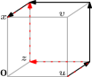
  (a) The case $|x|=1$.

  

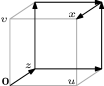
  (b) The case $|x|=2,u\sim x$.

  

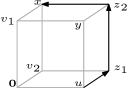
  (c) The case $|x|=2,|u-x|=3$.

  

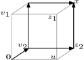
  (d) The case $|x|=3$.

  Figure 2: An illustration of several appearing cases for $|u|=1$. In the first two cases, $\mathbf{0}$ and $v$ are vacant in $\omega_{1}$. In case (a), the black path is $\gamma_{1}$, the red and dotted one is $\gamma_{2}$. In case (b), the two $\mathbf{0}$-$x$-paths are marked as black chains of arrows. In case (c), $\{v_{1},v_{2}\}\cap\omega_{0}=\{v_{1}\}$ and the only relevant $u$-$x$-path is marked in black.

  We now show that only $\gamma_{1}$ produces a relevant term. Assume first that $y_{2}\notin\omega_{1}$, but $\gamma_{2}\subseteq\omega_{1}$. For $E^{\prime}(u,x;\mathscr{C}_{0})_{1}$ to hold, $z\in\langle\mathscr{C}_{0}\rangle$ must not be a pivotal point. Under $\gamma_{2}\subseteq\omega_{1}$,

  $$\{z\notin\textsf{Piv}(u,x)\}_{1}\subseteq\bigcup_{a\in\{u,y_{1}\},b\in\{y_{3},x\}}\{a\longleftrightarrow b\text{ in }\omega_{1}\setminus\{z\}\}_{1}.$$ (5.8)

  Resolving the right-hand side of (5.8) by a union bound gives four connection events. The shortest $\omega_{1}$-path from $u$ to $x$ of non-vacant vertices is of length 4. Moreover, the shortest $\omega_{1}$-path from $y_{1}$ to $y_{3}$ of non-vacant vertices that avoids $z$ is of length $4$ as well, and so (5.7) is bounded by

  $$\Omega(\Omega-2)p_{c}\sum_{z} \mathbb{P}\Big{(}E^{\prime}(u,x;\mathscr{C}_{0})_{1},\{\mathbf{0},v,y_{2}\}\cap\omega_{1}=\varnothing,\gamma_{2}\subseteq\omega_{1}\Big{)}$$

  $$\leq\Omega^{3}p_{c}^{4}\Big{(}\tau^{(4)}(x-u)+\tau^{(3)}(y_{3}-u)+\tau^{(3)}(x-y_{1})+\tau^{(4)}(y_{3}-y_{1})\Big{)}=\mathcal{O}(\Omega^{-2}).$$

  We now show that $\gamma_{1}\in\omega_{1}$ gives a contribution. Note that under $\{\mathbf{0},v\notin\omega_{1},\gamma_{1}\subseteq\omega_{1}\}$,

  $$E^{\prime}(u,x;\mathscr{C}_{0})_{1}=\bigcap_{i\in\{1,2,3\}}\Big{(}\{y_{i}\notin\textsf{Piv}(u,x)\}_{1}\cup\{y_{i}\notin\langle\mathscr{C}_{0}\rangle\}_{0}\Big{)}$$ (5.9)

  But $\mathbb{P}(\{y_{i}\notin\textsf{Piv}(u,x)\}_{1}\cup\{y_{i}\notin\langle\mathscr{C}_{0}\rangle\}_{0})\geq 1-\mathbb{P}(y_{i}\in\langle\mathscr{C}_{0}\rangle)\geq 1-\tau^{(2)}(y_{i})=1-\mathcal{O}(\Omega^{-1})$ for all $i$ by Lemma 4.2, and so, by inclusion-exclusion,

  $$\Omega(\Omega-2)p_{c}\sum_{z} \mathbb{P}\Big{(}E^{\prime}(u,x;\mathscr{C}_{0})_{1},\{\mathbf{0},v\}\cap\omega_{1}=\varnothing,\gamma_{1}\subseteq\omega_{1}\Big{)}$$

  $$\begin{cases}\leq\Omega(\Omega-2)(\Omega-4)(1-p_{c})^{2}p_{c}^{4}\big{(}1-\mathcal{O}(\Omega^{-1})\big{)}=\Omega^{-1}+\mathcal{O}(\Omega^{-2}),\\ \geq\Omega^{3}p_{c}^{4}(1-\mathcal{O}(\Omega^{-1}))-\Omega^{2}\binom{\Omega-4}{2}p_{c}^{7}=\Omega^{-1}+\mathcal{O}(\Omega^{-2}).\end{cases}$$

• Let $x\neq\pm u,v\notin\omega_{1}$, and $\mathbf{0}\in\omega_{1}$. By Observation 4.3,

  $$\Omega p_{c}(\Omega-2)\mathbb{P}\big{(}E^{\prime}(u,x;\mathscr{C}_{0})_{1}\cap\{v\notin\omega_{1},\mathbf{0}\in\omega_{1}\}\big{)}\leq\Omega^{2}p_{c}^{2}\tau^{(4)}(x-u)=\mathcal{O}(\Omega^{-2}).$$

The case of $|u|=1,|x|=2$ contributes $\Omega^{2}p_{c}^{2}+\Omega^{-1}+\mathcal{O}(\Omega^{-2})$: There are $\tfrac{1}{2}\Omega^{2}$ choices for $x$. We first consider the $\Omega-1$ choices neighboring $u$ and, among those, exclude the special case $x=2u$ first. For $x$ a neighbor of $u$, we set $v:=x-u$.

• Let $x=2u$. Since $x\sim u$, we have $E^{\prime}(u,x;\mathscr{C}_{0})_{1}=\{x\in\langle\mathscr{C}_{0}\rangle\}_{0}\subseteq\{\mathbf{0}\xleftrightarrow{\,\,(4)\,\,}x\}_{0}$, and so the contribution to (5.7) is bounded by $\Omega p_{c}\tau^{(4)}(x)=\mathcal{O}(\Omega^{-2})$.

• Let $2u\neq x\sim u$ and $v\in\omega_{0}$. There are $\Omega-2$ choices for $x$. The event $E^{\prime}(u,x;\mathscr{C}_{0})_{1}$ holds, and so

  $$\Omega p_{c}\sum_{2u\neq x\sim u}\mathbb{E}_{0}\left[\mathds{1}_{\{v\in\omega_{0}\}}\mathbb{P}_{1}\left(E^{\prime}(u,x;\mathscr{C}_{0})\right)\right]=\Omega(\Omega-2)p_{c}^{2}=\Omega^{2}p_{c}^{2}-2\Omega^{-1}+\mathcal{O}(\Omega^{-2}).$$

• Let $2u\neq x\sim u$ and $v\notin\omega_{0}$. We partition

  $$E^{\prime}(u,x;\mathscr{C}_{0})_{1}=\Big{(}E^{\prime}(u,x;\mathscr{C}_{0})_{1}\cap\{\mathbf{0}\xleftrightarrow{\,\,(\leq 4)\,\,}x\text{ in }\mathbb{Z}^{d}\setminus\{u\}\}_{0}\Big{)}\cup\Big{(}E^{\prime}(u,x;\mathscr{C}_{0})_{1}\cap\{\mathbf{0}\xleftrightarrow{\,\,(\geq 6)\,\,}x\text{ in }\mathbb{Z}^{d}\setminus\{u\}\}_{0}\Big{)}$$

  and treat the second event by observing

  $$\Omega p_{c}\sum_{2u\neq x\sim u}\mathbb{P}\Big{(}\{v\notin\omega_{0}\}_{0}\cap\{\mathbf{0}\xleftrightarrow{\,\,(\geq 6)\,\,}x\text{ in }\mathbb{Z}^{d}\setminus\{u\}\}_{0}\cap E^{\prime}(u,x;\mathscr{C}_{0})_{1}\Big{)}\leq\Omega^{2}p_{c}\tau^{(6)}(x)=\mathcal{O}(\Omega^{-2}).$$

  As the only $2$-paths from $\mathbf{0}$ to $x$ go through $u$ and $v$ respectively, we can focus on paths of length $4$ avoiding $v$ and $u$. Hence, the status of $v$ is independent of such paths. Let $z$ be one of the $\Omega-4$ neighbors of $\mathbf{0}$ with $\dim\langle\!\langle u,v,z\rangle\!\rangle=3$. For any such $z$, there are two $\mathbf{0}$-$x$-paths of length $4$ that first visit $z$ and avoid $\{v,u\}$. More precisely, these paths are $(\mathbf{0},z,u+z,x+z,x)$ and $(\mathbf{0},z,v+z,x+z,x)$. Let $Q_{4}(z)$ denote the event that at least one of these paths is in $\omega_{0}$. See Figure 2(b) for an illustration. As the events $\{Q_{4}(z)\}$ are pairwise independent,

  $$\{v\notin\omega_{0}\}_{0}\cap\{\mathbf{0}\xleftrightarrow{\,\,(\leq 4)\,\,}x\text{ in }\mathbb{Z}^{d}\setminus\{u\}\}_{0}\cap E^{\prime}(u,x;\mathscr{C}_{0})_{1} =\{v\notin\omega_{0}\}_{0}\cap\big{(}\cup_{z}Q_{4}(z)\big{)},$$

  $$\mathbb{P}(\cup_{z}Q_{4}(z))=(\Omega-4)\mathbb{P}(Q_{4}(z))+\mathcal{O}(\Omega^{-4}) =2(\Omega-4)p_{c}^{3}+\mathcal{O}(\Omega^{-3}).$$

  Consequently,

  $$\Omega p_{c}\sum_{2u\neq x\sim u}\mathbb{P} \Big{(}\{v\notin\omega_{0}\}_{0}\cap\{\mathbf{0}\xleftrightarrow{\,\,(\leq 4)\,\,}x\text{ in }\mathbb{Z}^{d}\setminus\{u\}\}_{0}\cap E^{\prime}(u,x;\mathscr{C}_{0})_{1}\Big{)}$$

  $$=\Omega p_{c}(\Omega-2)2(\Omega-4)p_{c}^{3}+\mathcal{O}(\Omega^{-2})=2\Omega^{-1}+\mathcal{O}(\Omega^{-2}).$$

• Let $|u-x|=3$ and $\|x\|_{\infty}=2$. There are $\Omega-1$ choices for $x$. Let $2v=x$. Note first that

  $$\Omega(\Omega-1)p_{c}\mathbb{P}\Big{(} \big{(}\{x\in\langle\mathscr{C}_{0}\rangle\}_{0}\cup\{u\xleftrightarrow{\,\,(5)\,\,}x\}_{1}\big{)}\cap E^{\prime}(u,x;\mathscr{C}_{0})_{1}\Big{)}$$

  $$\leq\Omega^{2}p_{c}\Big{(}\tau^{(2)}(x)\tau^{(3)}(x-u)+\tau^{(5)}(x-u)\Big{)}=\mathcal{O}(\Omega^{-2}).$$

  The complementary event is that $x\notin\langle\mathscr{C}_{0}\rangle$ and the presence of a $u$-$x$-path of length $3$. The former implies $v\notin\omega_{0}$. There are at most four potential sites that can make up internal vertices on a $u$-$x$-path of length $3$, namely $\mathbf{0},v,u+v,u+2v$. To avoid potential pivotality of $\mathbf{0}$ and $v$ and still guarantee a path of length $3$, we require $\{v+u,v+2u\}\subseteq\omega_{1}$. But both these vertices are of distance at least $2$ from the origin, and at least one of them must be in $\langle\mathscr{C}_{0}\rangle$. In conclusion,

  $$\Omega(\Omega-1)p_{c}\mathbb{P}\Big{(} \{x\notin\langle\mathscr{C}_{0}\rangle\}_{0}\cap\{u\xleftrightarrow{\,\,(\leq 3)\,\,}x\}_{1}\cap E^{\prime}(u,x;\mathscr{C}_{0})_{1}\Big{)}$$

  $$\leq 2\Omega^{2}p_{c}\tau^{(2)}(u+v)\tau^{(3)}(x-u)=\mathcal{O}(\Omega^{-2}).$$

• Let $|u-x|=3,\|x\|_{\infty}=1$, and $x\in\langle\mathscr{C}_{0}\rangle$. Write $x=v_{1}+v_{2}$, where $|v_{i}|=1$. We first show that contributions arise when precisely one point in $\{v_{1},v_{2}\}$ is $\omega_{0}$-occupied. Note that when both $v_{1}$ and $v_{2}$ are vacant in $\omega_{0}$, the contribution to (5.7) is bounded by $\Omega^{3}p_{c}\tau^{(4)}(x)\tau^{(3)}(x-u)=\mathcal{O}(\Omega^{-2})$. On the other hand, if $\{v_{1},v_{2}\}\subseteq\omega_{0}$, then the contribution is bounded by $\Omega^{3}p_{c}^{3}\tau^{(3)}(u-x)=\mathcal{O}(\Omega^{-2})$.

  Let now $v_{1}\in\omega_{0}$ and $v_{2}\notin\omega_{0}$ (the other case is identical and is respected by counting the contribution twice). There are $\tfrac{1}{2}\Omega^{2}(1+\mathcal{O}(\Omega^{-1}))$ choices for $x$. If $\{u\xleftrightarrow{\,\,(5)\,\,}x\}_{1}$, then the contribution to (5.7) is $\mathcal{O}(\Omega^{-2})$. Set $z_{1}=u+v_{2},z_{2}=u+v_{2}+v_{1}$, and set $y=u+v_{1}$. We claim that the only $u$-$x$-path of length 3 that produces a relevant contribution is $(u,z_{1},z_{2},x)$. See Figure 2(c) for an illustration.

  First, assume $z_{1}\notin\omega_{1}$. Note that the only other paths of length $3$ from $u$ to $x$ go through either $\mathbf{0}$ or $y$. But $\{0,y\}\subseteq\langle\mathscr{C}_{0}\rangle$, and so neither $\mathbf{0}$ nor $y$ can be a pivotal point. Hence, $E^{\prime}(u,x;\mathscr{C}_{0})_{1}\cap\{z_{1}\notin\omega_{1}\}$ enforces $\{\mathbf{0},y\}\subseteq\omega_{1}$. To get to $x$ and avoid pivotality of any points in $\langle\mathscr{C}_{0}\rangle$, at least two points in $\{v_{1},v_{2},z_{1}\}$ must be occupied, and the contribution to (5.7) is at most

  $$2\Omega p_{c}\big{(}\tfrac{1}{2}\Omega^{2}(1+\mathcal{O}(\Omega^{-1}))\big{)}p_{c}^{2}\binom{3}{2}p_{c}^{2}=\mathcal{O}(\Omega^{-2}).$$

  If $z_{1}\in\omega_{1}$ and $z_{2}\notin\omega_{1}$, then the only $u$-$x$-path of length $3$ through $z_{1}$ visits $v_{2}\in\langle\mathscr{C}_{0}\rangle$. This gives a contribution of $\mathcal{O}(\Omega^{-2})$ by the same bound as above. We may turn to the case $z_{i}\in\omega_{1}$ for $i\in\{1,2\}$. Now, under $\{v_{1}\in\omega_{0},\{z_{1},z_{2}\}\subseteq\omega_{1}\}$, we can express $E^{\prime}(u,x;\mathscr{C}_{0})_{1}$ similarly to (5.9), replacing $y_{i}$ ($i\in[3]$) by $z_{i}$ ($i\in[2]$). Applying the same bounds, we obtain a contribution to (5.7) of

  $$2\Omega p_{c}\big{(}\tfrac{1}{2}\Omega^{2}(1+\mathcal{O}(\Omega^{-1}))\big{)}\mathbb{P}\big{(}v_{1}\in\omega_{0},\{z_{1},z_{2}\}\subseteq\omega_{1}\big{)}(1-\mathcal{O}(\Omega^{-1}))=\Omega^{-1}+\mathcal{O}(\Omega^{-2}).$$

• Let $|u-x|=3,\|x\|_{\infty}=1$, and $x\notin\langle\mathscr{C}_{0}\rangle$. Let $\gamma$ be a $u$-$x$-path in $\omega_{1}$. By assumption, there needs to be some $z\in\gamma$ with $z\in\langle\mathscr{C}_{0}\rangle$. Consequently, $z$ cannot be a pivotal point and so there needs to be another $u$-$x$-path $\tilde{\gamma}$ in $\omega_{1}$ that contains a point $\tilde{z}\notin\gamma$ with $\tilde{z}\in\langle\mathscr{C}_{0}\rangle$. Assume first that both $\gamma,\tilde{\gamma}$ are paths of length $3$. If they are disjoint, then the contribution to (5.7) is at most $9\Omega^{3}p_{c}^{5}=\mathcal{O}(\Omega^{-2})$. If they share their first vertex, then, in the terminology of Figure 2(c), it must be either $y$ or $z_{1}$ (otherwise $\mathbf{0}$ is pivotal). W.l.o.g., $\tilde{\gamma}$ must then pass through $z_{2}$ and so $\tilde{z}=z_{2}\in\langle\mathscr{C}_{0}\rangle$ needs to hold, and the contribution to (5.7) is at most $\Omega^{3}p_{c}^{4}\tau^{(3)}(z_{2})=\mathcal{O}(\Omega^{-2})$. Assume next that $\tilde{\gamma}$ is of length $5$. As $\gamma$ and $\tilde{\gamma}$ share at most one internal vertex (and there are two internal vertices in $\gamma$), we count a factor of $p_{c}$ for the unique vertex of $\gamma$, and the contribution to (5.7) is at most $18\Omega^{3}p_{c}^{2}\tau^{(5)}(x-u)=\mathcal{O}(\Omega^{-2})$. Similarly, when both $\gamma$ and $\tilde{\gamma}$ are of length at least $5$, the contribution is $\mathcal{O}(\Omega^{-2})$.

The case of $|u|=1,|x|=3$ contributes $2\Omega^{-1}+\mathcal{O}(\Omega^{-2})$: Note that when $\{u\xleftrightarrow{\,\,(4)\,\,}x\}_{1}$, then the contribution to (5.6) is at most

$$p_{c}\sum_{u,x}\triangle^{(8)}(u,x,\mathbf{0})+p_{c}^{2}\sum_{u,t,z,x}\triangleleft\triangleright^{(9)}(u,t,z,x)=\mathcal{O}(\Omega^{-2})$$ (5.10)

by Lemma 4.2. We can therefore focus on $x$ with $|x-u|=2$ and $\{u\xleftrightarrow{\,\,(=2)\,\,}x\}_{1}$. Moreover, we can assume that there is no $u$-$x$-path of length $4$. Let $x=u+v_{1}+v_{2}$, where $|v_{1}|=1=|v_{2}|$, and assume first that $\dim\langle\!\langle u,v_{1},v_{2}\rangle\!\rangle=3$. There are $\tfrac{1}{2}(\Omega-2)(\Omega-4)$ choices for $x$. Let $z_{i}=u+v_{i}$ be the two internal vertices of the two shortest $u$-$x$-paths—see Figure 2(d) for an illustration.

We first claim that only $x\in\langle\mathscr{C}_{0}\rangle$ produces a relevant contribution. Indeed, if $x\notin\langle\mathscr{C}_{0}\rangle$, and as there is no $u$-$x$-path of length $4$, we must have $z_{i}\in\omega_{1}\cap\langle\mathscr{C}_{0}\rangle$ for $i\in\{1,2\}$. For $\{\mathbf{0}\longleftrightarrow z_{i}\}_{0}$ to hold, either $v_{i}\in\omega_{0}$, or $\{\mathbf{0}\xleftrightarrow{\,\,(4)\,\,}z_{i}\}_{0}$, and so (5.7) is at most

$$\Omega^{3}p_{c}\mathbb{P} \Big{(}\{\{z_{1},z_{2}\}\subseteq\omega_{1}\}\cap\big{(}\{\{v_{1},v_{2}\}\subseteq\omega_{0}\}\cup\{\mathbf{0}\xleftrightarrow{\,\,(4)\,\,}z_{1}\}_{0}\cup\{\mathbf{0}\xleftrightarrow{\,\,(4)\,\,}z_{2}\}_{0}\big{)}\Big{)}$$

$$=\Omega^{3}p_{c}^{3}\big{(}p_{c}^{2}+\tau^{(4)}(z_{1})+\tau^{(4)}(z_{2})\big{)}=\mathcal{O}(\Omega^{-2}).$$

Turning to $x\in\langle\mathscr{C}_{0}\rangle$, note that when $\{z_{1},z_{2}\}\subseteq\omega_{1}$, then (5.7) is at most

$$\Omega^{3}p_{c}\mathbb{P}\big{(}\{\mathbf{0}\longleftrightarrow x\}_{0}\cap\{\{z_{1},z_{2}\}\subseteq\omega_{1}\}\big{)}=\Omega^{3}p_{c}^{3}\tau^{(3)}(x)=\mathcal{O}(\Omega^{-2}).$$

W.l.o.g., we assume that $z_{1}\in\omega_{1}$ (and $z_{2}\notin\omega_{1}$) and (by symmetry) count the contribution twice. Now, the contribution to (5.7) is equal to

$$\Omega(\Omega-2)(\Omega-4)p_{c}\mathbb{P}\Big{(}\{x\in\langle\mathscr{C}_{0}\rangle\}_{0}\cap\{z_{2}\notin\omega_{1}\ni z_{1}\}_{1}\cap\big{(}\{z_{1}\notin\langle\mathscr{C}_{0}\rangle_{0}\cup\{z_{1}\notin\textsf{Piv}(u,x)\}_{1}\big{)}\Big{)}.$$ (5.11)

If $v_{1}\in\omega_{0}$, then $z_{1}\in\langle\mathscr{C}_{0}\rangle$ and so $z_{1}$ cannot be pivotal, which, in turn, forces $\{u\xleftrightarrow{\,\,(4)\,\,}x\}_{1}$. But this was already shown to produce an $\mathcal{O}(\Omega^{-2})$ contribution. Further, if $\{\mathbf{0}\xleftrightarrow{\,\,(5)\,\,}x\}_{0}$, then (5.11) is at most $\Omega^{3}p_{c}^{2}\tau^{(5)}(x)=\mathcal{O}(\Omega^{-2})$, and so $\mathbf{0}$ must be $\omega_{0}$-connected to $x$ by a path of length $3$.

There are precisely two $\mathbf{0}$-$x$-paths of length 3 that use neither $v_{1}$ nor $u$, namely $\gamma_{1}=(\mathbf{0},v_{2},v_{1}+v_{2},x)$ and $\gamma_{2}=(\mathbf{0},v_{2},z_{2},x)$. If both are occupied, the contribution is $\mathcal{O}(\Omega^{-2})$. Note that

$$\mathbb{P}(z_{1}\notin\langle\mathscr{C}_{0}\rangle\mid\gamma_{i}\subseteq\omega_{0})\geq 1-3\tau^{(2)}(z_{1})=1-\mathcal{O}(\Omega^{-1}),$$

and so (5.11) becomes

$$\Omega^{3}(1-\mathcal{O}(\Omega^{-1}))p_{c}\mathbb{P}\Big{(}\big{(}\cup_{i=1,2}\{\gamma_{i}\subseteq\omega_{0}\}_{0}\big{)},z_{1}\in\omega_{1}\Big{)}=2\Omega^{3}p_{c}^{4}(1-\mathcal{O}(\Omega^{-1}))=2\Omega^{-1}+\mathcal{O}(\Omega^{-2}).$$

Finally, if $\dim\langle\!\langle u,v_{1},v_{2}\rangle\!\rangle\leq 2$, then the same bounds with at least one factor of $\Omega$ in the choice of $x$ gives a contribution of $\mathcal{O}(\Omega^{-2})$.

The case of $|u|=1,|x|\geq 4$ contributes $\mathcal{O}(\Omega^{-2})$: The bound is the same as in (5.10).

Contributions of $|u|=2$.

If $u$ is one of the $\Omega$ points with $|u|=2=\|u\|_{\infty}$, then $\widehat{\Pi}^{(1)}$ is bounded by $\Omega p_{c}\sum_{x}\mathbb{P}(\mathbf{0}\Longleftrightarrow u)\tau_{p}(u-x)$. For fixed $j=|u-x|$, this is bounded by

$$\Omega^{1+j}p_{c}\tau^{(2)}(u)\tau^{(4)}(u)\tau^{(j)}(x-u)=\mathcal{O}(\Omega^{-2}).$$

We now show that we can impose some further restrictions on $u$ and $x$. Recall the bound in (5.5), and observe that if $x\notin\langle\mathscr{C}_{0}\rangle$, then

$$p_{c}\sum_{|u|=2}\sum_{x}\mathbb{P}\big{(}\{\mathbf{0}\Longleftrightarrow u\}_{0}\cap\{x\notin\langle\mathscr{C}_{0}\rangle\}_{0}\cap E^{\prime}(u,x;\mathscr{C}_{0})_{1}\big{)}\leq p_{c}^{2}\sum\mathds{1}_{\{|u|=2\}}\mathrel{\raisebox{-7.11317pt}{\includegraphics{N1_exp_A_general_labels.pdf}}}\ =\mathcal{O}(\Omega^{-2}).$$

Similar considerations enforce that $|x|\leq 3$ and $|x-u|\leq 2$ as well as $\{\mathbf{0}\xLeftrightarrow{\,\,(\leq 4)\,\,}u\}_{0}$. Before going into the different cases, we note that there are $\tfrac{1}{2}\Omega(\Omega-2)$ choices for $u=v_{1}+v_{2}$ (where $|v_{i}|=1$), and on every choice, $\{v_{1},v_{2}\}\subseteq\omega_{0}$ need to hold for a relevant contribution to arise. Taking all this into consideration, the contribution to $\widehat{\Pi}^{(1)}$ becomes

$$\tfrac{1}{2}\Omega(\Omega-2)p_{c}^{3}\sum_{x\in\mathbb{Z}^{d}}\mathds{1}_{\{|x|\leq 3,|u-x|\leq 2\}}\mathbb{P}\Big{(}\{x\in\langle\mathscr{C}_{0}\rangle\}_{0}\cap E^{\prime}(u,x;\mathscr{C}_{0})_{1}\mid\{v_{1},v_{2}\}\subseteq\omega_{0}\Big{)},$$ (5.12)

where $v_{1}$ and $v_{2}$ is a pair of arbitrary but fixed independent unit vectors (and $u=v_{1}+v_{2}$).

The case of $|u|=2,x=\mathbf{0}$ contributes $\mathcal{O}(\Omega^{-2})$: As $|u-x|=2$, the contribution to (5.12) is at most $\Omega^{2}p_{c}^{3}\tau^{(2)}(x-u)=\mathcal{O}(\Omega^{-2})$.

The case of $|u|=2,|x|=1$ contributes $\Omega^{-1}+\mathcal{O}(\Omega^{-2})$: Note that we only need to consider $x\in\{v_{1},v_{2}\}$ (otherwise $|u-x|=3$). For these choices of $x$, both $x\in\langle\mathscr{C}_{0}\rangle$ and $E^{\prime}(u,x;\mathscr{C}_{0})_{1}$ hold and the contribution to (5.12) is as claimed.

The case of $|u|=2,|x|=2$ contributes $\Omega^{-1}+\mathcal{O}(\Omega^{-2})$: By the indicator in (5.12), we only consider $|x-u|=2$. Let first $\|x\|_{\infty}=2$. There are only two such points at distance $2$ of $u$, and so the contribution to (5.12) is at most $\Omega^{2}p_{c}^{3}\tau^{(2)}(x-u)=\mathcal{O}(\Omega^{-2})$.

Let thus $x$ be one of the $2(\Omega-3)$ points with $\|x\|_{\infty}=1$. W.l.o.g., we assume that $x=v_{1}+v_{3}$, where $|v_{3}|=1$. If $v_{3}=-v_{2}$, then the contribution is bounded by $\Omega^{2}p_{c}^{3}\tau^{(2)}(x-u)=\mathcal{O}(\Omega^{-2})$. Let $x$ be one of the remaining $2(\Omega-4)$ points with $\dim\langle\!\langle v_{1},v_{2},v_{3}\rangle\!\rangle=3$. As $x\sim v_{1}$, the event $x\in\langle\mathscr{C}_{0}\rangle$ holds. We partition $E^{\prime}(u,x;\mathscr{C}_{0})_{1}$ into whether $\{u\xleftrightarrow{\,\,(=2)\,\,}x\}_{1}$ or $\{u\xleftrightarrow{\,\,(\geq 4)\,\,}x\}_{1}$ and see that in the latter case, the contribution to (5.12) is at most $\Omega^{3}p_{c}^{3}\tau^{(4)}(x-u)=\mathcal{O}(\Omega^{-2})$.

For the existence of a path of length $2$, either $v_{1}$ or $v_{4}:=x+v_{2}$ need to be $\omega_{1}$-occupied. As $v_{1}\in\mathscr{C}_{0}$, it cannot be a pivotal point for the $\omega_{1}$-connection between $u$ and $x$ and there needs to be another path. The contribution to (5.12) is therefore at most $\Omega^{3}p_{c}^{4}\tau^{(2)}(x-u)=\mathcal{O}(\Omega^{-2})$. We observe that

$$E^{\prime}(u,x;\mathscr{C}_{0})_{1}\cap\{v_{4}\in\omega_{1}\}=\{v_{4}\in\omega_{1}\}\cap\Big{(}\{v_{4}\notin\textsf{Piv}(u,x)\}_{1}\cup\{\mathbf{0}\centernot\longleftrightarrow v_{4}\text{ in }\mathbb{Z}^{d}\setminus\{u\}\}_{0}\Big{)}.$$

As previously, $\mathbb{P}(v_{4}\notin\textsf{Piv}(u,x))=\mathcal{O}(\Omega^{-1})$ and $\mathbb{P}(\mathbf{0}\centernot\longleftrightarrow v_{4}\text{ in }\mathbb{Z}^{d}\setminus\{u\})=1-\mathcal{O}(\Omega^{-1})$, and so the contribution to (5.12) is

$$\Omega^{3}(1-\mathcal{O}(\Omega^{-1}))p_{c}^{4}(1+\mathcal{O}(\Omega^{-1}))=\Omega^{-1}+\mathcal{O}(\Omega^{-2}).$$

The case of $|u|=2,|x|=3$ contributes $\Omega^{-1}+\mathcal{O}(\Omega^{-2})$: We only need to consider neighbors of $u$, otherwise $|u-x|\geq 3$. Recall that for $|u-x|=1$, the event $E^{\prime}(u,x;\mathscr{C}_{0})_{1}$ holds precisely when $x\in\langle\mathscr{C}_{0}\rangle$. Under our conditioning, $x$ must be connected to $\{0,v_{1},v_{2}\}$. Note that there are two choices for $x$ with $\|x\|_{\infty}=2$. Since $\mathbb{P}(x\in\langle\mathscr{C}_{0}\rangle)\leq 3\max_{y\in\{0,v_{1},v_{2}\}}\tau^{(2)}(x-y))=\mathcal{O}(\Omega^{-1})$, we may focus on the $\Omega-2$ choices of $x$ with $\|x\|_{\infty}=1$.

Let $x=u+v_{3}$ and set $z_{1}:=v_{1}+v_{3},z_{2}:=v_{2}+v_{3}$. If $\{z_{1},z_{2}\}\cap\omega_{0}=\varnothing$, then $\{\mathbf{0}\xleftrightarrow{\,\,(5)\,\,}x\}_{0}$ holds, and the contribution to (5.12) is at most $\Omega^{3}p_{c}^{3}\max_{y\in\{0,v_{1},v_{2}\}}\tau^{(3)}(x-y)=\mathcal{O}(\Omega^{-2})$. If $\{z_{1},z_{2}\}\subset\omega_{0}$, then the contribution to (5.12) is at most $\Omega^{3}p_{c}^{5}=\mathcal{O}(\Omega^{-2})$.

We consider the case where $z_{1}\notin\omega_{0}\ni z_{2}$ and respect the other case with a factor of $2$. The contribution to (5.12) is

$$\Omega^{3}(1+\mathcal{O}(\Omega^{-1})p_{c}^{4}(1+\mathcal{O}(\Omega^{-1}))=\Omega^{-1}+\mathcal{O}(\Omega^{-2}).$$

This finishes the analysis of $\widehat{\Pi}^{(1)}$. ∎

5.3 Analysis of $\widehat{\Pi}^{(2)}$

Lemma 5.3 (Asymptotics of $\widehat{\Pi}^{(2)}$).

As $d\to\infty$,

$$\widehat{\Pi}^{(2)}=10\Omega^{-1}+\mathcal{O}(\Omega^{-2}).$$

Proof.

For the proof, we recall that

$$\widehat{\Pi}^{(2)}=p_{c}^{2}\sum_{u,v,x\in\mathbb{Z}^{d}}\mathbb{P}\Big{(}\{\mathbf{0}\Longleftrightarrow u\}_{0}\cap E^{\prime}(u,v;\mathscr{C}_{0})_{1}\cap E^{\prime}(v,x;\mathscr{C}_{1})_{2}\Big{)},$$ (5.13)

where $\mathscr{C}_{0}=\widetilde{\mathscr{C}}^{u}(\mathbf{0};\omega_{0})$ and $\mathscr{C}_{1}=\widetilde{\mathscr{C}}^{v}(u;\omega_{1})$. We first show that when either $v\notin\langle\mathscr{C}_{0}\rangle$ or $x\notin\langle\mathscr{C}_{1}\rangle$, then the contribution to $\widehat{\Pi}^{(2)}$ is $\mathcal{O}(\Omega^{-2})$. Indeed, by Lemma 2.10 and Proposition 2.8,

$$p_{c}^{2}\sum_{u,v,x\in\mathbb{Z}^{d}}\mathbb{P} \Big{(}\{\mathbf{0}\Longleftrightarrow u\}_{0}\cap E^{\prime}(u,v;\mathscr{C}_{0})_{1}\cap E^{\prime}(v,x;\mathscr{C}_{1})_{2}\cap\big{(}\{v\notin\langle\mathscr{C}_{0}\rangle\}_{0}\cup\{x\notin\langle\mathscr{C}_{1}\rangle\}_{1}\big{)}\Big{)}$$

$$\leq p_{c}^{2}\sum\Big{(}p_{c}^{3}\mathrel{\raisebox{-7.11317pt}{\includegraphics{N2_exp_11.pdf}}}+p_{c}^{2}\mathrel{\raisebox{-7.11317pt}{\includegraphics{N2_exp_12.pdf}}}$$

$$\qquad+p_{c}^{2}\mathrel{\raisebox{-7.11317pt}{\includegraphics{N2_exp_21.pdf}}}+p_{c}\mathrel{\raisebox{-7.11317pt}{\includegraphics{N2_exp_31.pdf}}}+p_{c}\mathrel{\raisebox{-7.11317pt}{\includegraphics{N2_exp_22.pdf}}}\Big{)}$$ (5.14)

$$\leq\sum\mathrel{\raisebox{-7.11317pt}{\includegraphics{N1_exp_A_bound1.pdf}}}\Big{(}\triangle_{p_{c}}^{\bullet}(\triangle_{p_{c}}^{\bullet\circ})^{2}\triangle_{p_{c}}+\triangle_{p_{c}}^{\bullet}\triangle_{p_{c}}\triangle_{p_{c}}^{\bullet\circ}+\triangle_{p_{c}}^{\bullet}\triangle_{p_{c}}^{\bullet\circ}\triangle_{p_{c}}^{\bullet\bullet\circ}\triangle_{p_{c}}+\triangle_{p_{c}}^{\bullet}(\triangle_{p_{c}}^{\bullet\circ})^{2}\Big{)}$$

$$\qquad+p_{c}^{3}\sum\Big{(}p_{c}\mathrel{\raisebox{-7.11317pt}{\includegraphics{N2_exp_22nocoll.pdf}}}+\mathrel{\raisebox{-7.11317pt}{\includegraphics{N2_exp_22coll.pdf}}}\Big{)}$$ (5.15)

$$\leq\mathcal{O}(\Omega^{-3})\sum\mathrel{\raisebox{-7.11317pt}{\includegraphics{N1_exp_A_bound1.pdf}}}\ =\mathcal{O}(\Omega^{-2}).$$

We expanded the third diagram in (5.14) to get the two diagrams of (5.15). We next show that only $|u|=1$ gives a relevant contribution. Indeed,

$$p_{c}^{2}\sum_{u,v,x\in\mathbb{Z}^{d}:|u|\geq 2}\mathbb{P} \Big{(}\{\mathbf{0}\Longleftrightarrow u\}_{0}\cap E^{\prime}(u,v;\mathscr{C}_{0})_{1}\cap E^{\prime}(v,x;\mathscr{C}_{1})_{2}\cap\{v\in\langle\mathscr{C}_{0}\rangle\}_{0}\cap\{x\in\langle\mathscr{C}_{1}\rangle\}_{1}\Big{)}$$

$$\leq p_{c}^{2}\sum\mathds{1}_{\{|u|\geq 2\}}\mathrel{\raisebox{-7.11317pt}{\includegraphics{N2_exp_32.pdf}}}\ \leq\triangle_{p_{c}}^{\bullet}\triangle_{p_{c}}^{\bullet\circ}\sum\mathds{1}_{\{|u|\geq 2\}}\mathrel{\raisebox{-7.11317pt}{\includegraphics{N1_exp_A_bound1.pdf}}}\ =\mathcal{O}(\Omega^{-2}).$$

We can thus fix $u$ to be an arbitrary neighbor of the origin and need to investigate

$$\Omega p_{c}^{2}\sum_{v,x\in\mathbb{Z}^{d}}\mathbb{P}\Big{(}E^{\prime}(u,v;\mathscr{C}_{0})_{1}\cap E^{\prime}(v,x;\mathscr{C}_{1})_{2}\cap\{v\in\langle\mathscr{C}_{0}\rangle\}_{0}\cap\{x\in\langle\mathscr{C}_{1}\rangle\}_{1}\Big{)}.$$ (5.16)

Before going into specific cases, we exclude some of them right away: When $|x|\vee|u-x|\geq 4$, then the contribution to (5.16) is

$$p_{c}^{2}\sum\mathds{1}_{\{|x|\vee|u-x|\geq 4\}}\mathrel{\raisebox{-7.11317pt}{\includegraphics{N2_exp_32_u1.pdf}}}\ \leq\sum_{u,t,v,x}\triangleleft\triangleright^{(9)}(u,t,v,x)=\mathcal{O}(\Omega^{-2})$$

by Lemma 4.2. In the above, a line decorated with a ‘$\sim$’ symbol denotes a direct edge. Similarly, when $|v|\geq 3$ or $|x-v|\geq 3$, the contribution to (5.16) is at most

$$p_{c}^{2}\sum \mathds{1}_{\{|v|\vee|x-v|\geq 3\}}\mathrel{\raisebox{-7.11317pt}{\includegraphics{N2_exp_32_u1.pdf}}}\ \leq p_{c}\triangle_{p_{c}}^{\bullet}\big{(}\tau^{(3)}\ast\tau\ast\tau^{\bullet}\ast J\big{)}(\mathbf{0})+p_{c}^{2}\sum\mathds{1}_{\{|x-v|\geq 3\}}\mathrel{\raisebox{-7.11317pt}{\includegraphics{N2_exp_32_u1_subst.pdf}}}$$

$$\leq p_{c}\triangle_{p_{c}}^{\bullet}\sum_{u,v}\triangle^{(6)}(\mathbf{0},u,v)+p_{c}^{4}\big{(}J^{\ast 3}\ast\tau^{\ast 3}\big{)}(\mathbf{0})+p_{c}\triangle_{p_{c}}^{\bullet\circ}\sum_{t,x}\triangle^{(6)}(\mathbf{0},t,x)=\mathcal{O}(\Omega^{-2}).$$

We now investigate (5.16) by splitting the double sum over $v$ and $x$. We organize this by considering the three main cases for $|v|\in\{0,1,2\}$. An overview of the contributions is given in the following table:

$\widehat{\Pi}^{(2)}$:	$x=\mathbf{0}$	$|x|=1$	$|x|=2$	$|x|=3$
$v=\mathbf{0}$		$2\Omega^{-1}$	$\Omega^{-1}$
$|v|=1$	$\Omega^{-1}$		$2\Omega^{-1}$	$\Omega^{-1}$
$|v|=2$		$\Omega^{-1}$	$\Omega^{-1}$	$\Omega^{-1}$

Contributions of $v=\mathbf{0}$.

The events $E^{\prime}(u,v;\mathscr{C}_{0})_{1}$ and $\{v\in\langle\mathscr{C}_{0}\rangle\}$ hold.

The case of $|x|=1$ contributes $2\Omega^{-1}+\mathcal{O}(\Omega^{-2})$: First, consider the choice of $x=u$. It is easy to see that the event in (5.16) holds and the contribution is $\Omega p_{c}^{2}=\Omega^{-1}+\mathcal{O}(\Omega^{-2})$.

Consider $0\sim x\neq u$. As $v\sim x$, we have $E^{\prime}(v,x;\mathscr{C}_{1})_{2}=\{x\in\langle\mathscr{C}_{1}\rangle\}_{1}$. If $x=-u$, then $\{x\in\langle\mathscr{C}_{1}\rangle\}_{1}\subseteq\{u\xleftrightarrow{\,\,(4)\,\,}x\}_{1}$ and we receive a contribution of order $\mathcal{O}(\Omega^{-2})$. Consider now one of the $\Omega-2$ remaining choices for $x$ and set $z=u+x$. Then

$$\mathbb{P}(x\in\langle\mathscr{C}_{1}\rangle)=\mathbb{P}(z\in\omega_{1})+\mathbb{P}(z\notin\omega_{1},x\in\langle\mathscr{C}_{1}\rangle)=p_{c}+\mathcal{O}(\tau^{(4)}(x-u))=p_{c}+\mathcal{O}(\Omega^{-2}),$$

yielding a contribution to (5.16) of $\Omega(\Omega-2)p_{c}^{3}+\mathcal{O}(\Omega^{-2})=\Omega^{-1}+\mathcal{O}(\Omega^{-2})$.

The case of $|x|=2$ contributes $\Omega^{-1}+\mathcal{O}(\Omega^{-2})$: If $|u-x|=3$, then the contribution to (5.16) is bounded by $\Omega^{3}p_{c}^{2}\tau^{(2)}(x-v)\tau^{(3)}(u-x)=\mathcal{O}(\Omega^{-2})$. Similarly, if $x=2u$, we obtain a bound of $\Omega p_{c}^{2}\tau^{(2)}(x-v)=\mathcal{O}(\Omega^{-2})$. Let therefore $x$ be one of the $\Omega-2$ remaining neighbors of $u$ and note that $\{x\in\langle\mathscr{C}_{1}\rangle\}$ holds.

We set $z=x-u$. If $z\notin\omega_{2}$, then $E^{\prime}(v,x;\mathscr{C}_{1})_{2}\subseteq\{v\xleftrightarrow{\,\,(4)\,\,}x\}_{2}$ by Observation 4.3, and the contribution to (5.16) is at most $\Omega^{2}p_{c}^{2}\tau^{(4)}(x-v)=\mathcal{O}(\Omega^{-2})$. If $z\in\omega_{2}$, then $E^{\prime}(v,x;\mathscr{C}_{1})_{2}=\{z\notin\textsf{Piv}(v,x)\}_{2}\cup\{z\notin\langle\mathscr{C}_{1}\rangle\}_{1}$. By a similar argument to the one below (5.9), the contribution to (5.16) becomes

$$\Omega(\Omega-2)p_{c}^{2}\mathbb{P}\Big{(}\{z\in\omega_{2}\}\cap\big{(}\{z\notin\textsf{Piv}(v,x)\}_{2}\cup\{z\notin\langle\mathscr{C}_{1}\rangle\}_{1}\big{)}\Big{)}=\Omega^{2}p_{c}^{3}(1-\mathcal{O}(\Omega^{-1}))=\Omega^{-1}+\mathcal{O}(\Omega^{-2}).$$

The case of $|x|=3$ contributes $\mathcal{O}(\Omega^{-2})$: Distinguishing between $|u-x|=4$ (at most $\Omega^{3}$ choices for $x$) and $|u-x|=2$ (at most $\Omega^{2}$ choices), the contribution to (5.16) is at most

$$\Omega p_{c}^{2}\tau^{(3)}(x-v)\big{(}\Omega^{3}\tau^{(4)}(u-x)+\Omega^{2}\tau^{(2)}(u-x)\big{)}=\mathcal{O}(\Omega^{-2}).$$

Contributions of $|v|=1$.

Let us first consider $v=-u$ and show that this case contributes $\mathcal{O}(\Omega^{-2})$. Indeed, $E^{\prime}(u,v;\mathscr{C}_{0})_{1}\subseteq\{u\xleftrightarrow{\,\,(4)\,\,}v\}_{1}$ by Observation 4.3. With the further inclusion $E^{\prime}(v,x;\mathscr{C}_{1})_{2}\cap\{x\in\langle\mathscr{C}_{1}\rangle\}\subseteq\{v\longleftrightarrow x\}_{2}$, we have that the contribution to (5.16) is at most

$$\Omega p_{c}^{2}\tau^{(4)} (u-v)\Big{(}\sum_{|x|=1}\tau^{(2)}(x-v)+\sum_{x:v\sim x}1+\sum_{|x|=2,|x-v|=3}\tau^{(3)}(x-v)$$

$$\qquad+\sum_{|x|=3,|x-v|=2}\tau^{(2)}(x-v)+\sum_{|x|=3,|x-v|=4}\tau^{(4)}(x-v)\Big{)}$$

$$\leq\mathcal{O}(\Omega^{-3})\Big{(}\Omega\mathcal{O}(\Omega^{-1})+\Omega+\Omega^{2}\mathcal{O}(\Omega^{-2})+\Omega^{2}\mathcal{O}(\Omega^{-1})+\Omega^{3}\mathcal{O}(\Omega^{-3})\Big{)}=\mathcal{O}(\Omega^{-2}).$$

We may therefore take $v\neq\pm u$ to be one of the $\Omega-2$ remaining neighbors of the origin. Set $t=v+u$. We first claim that $t\notin\omega_{1}$ results in an $\mathcal{O}(\Omega^{-2})$ contribution. Note that, by Observation 4.3, $E^{\prime}(u,v;\mathscr{C}_{0})_{1}\cap\{t\notin\omega_{1}\}\subseteq\{u\xleftrightarrow{\,\,(4)\,\,}v\}_{1}$. As there is only one choice of $x$ such that $u\sim x\sim v$ and at most $\Omega$ choices such that $|x|=3$ and $x\sim v$, we can bound  (5.16) by

$$\Omega^{2}p_{c}^{2}\sum_{x\in\mathbb{Z}^{d}} \Big{(}\tau^{(4)}(v-u)\big{(}\mathds{1}_{\{x=\mathbf{0}\}}+\mathds{1}_{\{|x|=1\}}\tau^{(2)}(x-v)+\mathds{1}_{\{|x|=2,u\sim x\sim v\}}$$

$$\quad+\mathds{1}_{\{|x|=3,|u-x|=2=|v-x|\}}\tau^{(2)}(x-v)\big{)}+\mathds{1}_{|x|=2,v\sim x}\mathbb{P}\big{(}E^{\prime}(u,v;\mathscr{C}_{0})_{1}\cap\{t\notin\omega_{1}\}\cap\{x\in\langle\mathscr{C}_{1}\rangle\}\big{)}\Big{)}$$

$$\leq \mathcal{O}(\Omega^{-2})\big{(}2+2\Omega\tau^{(2)}(x-v)\big{)}+\mathcal{O}(1)\sum_{|x|=2,x\sim v}\mathbb{P}^{(2)}\big{(}E^{\prime}(u,v;\mathscr{C}_{0})_{1}\cap\{t\notin\omega_{1}\}\cap\{x\in\langle\mathscr{C}_{1}\rangle\}\big{)}.$$

It remains to bound the last probability. There are at most $\Omega$ choices for $x$. If $\{u\xleftrightarrow{\,\,(5)\,\,}x\}$, then the contribution is $\mathcal{O}(\Omega^{-2})$. Note that the $u$-$v$-path in $\omega_{1}$ cannot use and is independent of the status of $\mathbf{0}$, as the origin may not be a pivotal point. Hence, if $\mathbf{0}\in\omega_{1}$, the contribution is at most $\Omega p_{c}\tau^{(4)}(v-u)=\mathcal{O}(\Omega^{-2})$. We therefore assume $\mathbf{0}\notin\omega_{1}$ and aim to bound

$$\Omega\mathbb{P}\big{(}\{u\xleftrightarrow{\,\,(4)\,\,}v\}_{1}\cap\{\mathbf{0},t\notin\omega_{1}\}\cap\{u\xleftrightarrow{\,\,(\leq 3)\,\,}x\}_{1}\big{)}$$ (5.17)

When avoiding $\mathbf{0}$ and $t$, there are only two $u$-$x$-paths of length $3$, namely $\gamma_{1}=(u,y,z,x)$ and $\gamma_{2}=(u,y,y-u,x)$, where $y:=x+u-v$ and $z:=y+v$. See Figure 3(a) for an illustration. But now, (5.17) is bounded by

$$\Omega\mathbb{P}\Big{(} \{\mathbf{0},t\notin\omega_{1}\}\cap\bigcup_{i=1,2}\bigcup_{s\in\gamma_{i}\setminus\{x\}}\{\gamma_{i}\subseteq\omega_{1}\}\circ\{s\longleftrightarrow v\}_{1}\Big{)}$$

$$\leq 2\Omega p_{c}^{2}\big{(}\tau^{(4)}(v-u)+\tau^{(3)}(y-v)+2\tau^{(2)}(z-v)\big{)}=\mathcal{O}(\Omega^{-2}).$$

As a consequence, we can focus on $t\in\omega_{1}$, and (5.16) reduces to

$$\Omega(\Omega-2)p_{c}^{2}\sum_{x\in\mathbb{Z}^{d}}\mathbb{P}\Big{(}E^{\prime}(u,v;\mathscr{C}_{0})_{1}\cap E^{\prime}(v,x;\mathscr{C}_{1})_{2}\cap\{t\in\omega_{1},x\in\langle\mathscr{C}_{1}\rangle\}_{1}\Big{)}.$$

But under $t\in\omega_{1}$, we have $E^{\prime}(u,v;\mathscr{C}_{0})_{1}=\{t\notin\textsf{Piv}(u,v)\}_{1}\cup\{t\notin\langle\mathscr{C}_{0}\rangle\}_{0}$. The latter event has probability $1-\mathcal{O}(\Omega^{-1})$, and so we can can instead investigate

$$\Omega^{2}p_{c}^{2}(1-\mathcal{O}(\Omega^{-1}))\sum_{x\in\mathbb{Z}^{d}}\mathbb{P}\Big{(}E^{\prime}(v,x;\mathscr{C}_{1})_{2}\cap\{t\in\omega_{1},x\in\langle\mathscr{C}_{1}\rangle\}_{1}\Big{)},$$ (5.18)

where $u$ and $v$ are two arbitrary (but fixed) neighbors of $\mathbf{0}$ (satisfying ($u\neq\pm v$).

The contribution of $x=\mathbf{0}$ is $\Omega^{-1}+\mathcal{O}(\Omega^{-2})$: Note that $x\in\langle\mathscr{C}_{1}\rangle$ holds, and so does $E^{\prime}(v,x;\mathscr{C}_{1})_{2}$. Hence, the contribution to (5.18) is $\Omega^{-1}+\mathcal{O}(\Omega^{-2})$.

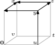
(a) The case $|x|=2,t\notin\omega_{1}$.

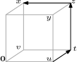
(b) The case $|x|=2,u\nsim x$.

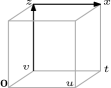
(c) The case $|x|=3$.

Figure 3: An illustration of several appearing cases for $|v|=1$. In (a), the two paths from $u$ to $x$ of length $3$ that avoid $\mathbf{0}$ and $t$ are drawn. In (b), the path along $t,z$ which ensures $x\in\langle\mathscr{C}_{1}\rangle$ for a contribution of $\Omega^{-1}$ is drawn. In (c), the scenario $|x-u|=2=|v-x|$ is shown, and the path along $z$ ensuring $\{v\longleftrightarrow x\}_{2}$ is drawn in black.

The contribution of $|x|=1$ is $\mathcal{O}(\Omega^{-2})$: If $x\in\{\pm u,-v\}$, we can bound the contribution to (5.18) by $\Omega^{2}p_{c}^{2}\tau^{(2)}(u-v)\tau^{(2)}(x-v)=\mathcal{O}(\Omega^{-2})$ (as both $\{v\longleftrightarrow x\}_{2}$ and $\{u\longleftrightarrow v\}_{1}$ need to hold). Consider thus one of the $\Omega-4$ choices for $x$ satisfying $\dim\langle\!\langle u,v,x\rangle\!\rangle=3$. Conditional on $t\in\omega_{1}$, we have $\{x\in\langle\mathscr{C}_{1}\rangle\}_{1}\subseteq\{u\xleftrightarrow{\,\,(2)\,\,}x\}_{1}\cup\{t\xleftrightarrow{\,\,(3)\,\,}x\}_{1}$, and so the contribution is at most

$$\Omega^{3}p_{c}^{3}\tau_{p}^{(2)}(x-v)\big{(}\tau_{p}^{(2)}(x-u)+\tau_{p}^{(3)}(x-t)\big{)}=\mathcal{O}(\Omega^{-2}).$$

The contribution of $|x|=2$ is $2\Omega^{-1}+\mathcal{O}(\Omega^{-2})$: We can restrict to the choices of $x$ where $v\sim x$ by the considerations made in the beginning of the proof.

• Let $x\sim u$. There is only one choice for $x$ such that $|u-x|=|v-x|=1$, namely $x=t$. For this choice, $E^{\prime}(v,x;\mathscr{C}_{1})_{2}$ certainly holds, and also $x\in\langle\mathscr{C}_{1}\rangle$. We get a contribution of $\Omega^{-1}+\mathcal{O}(\Omega^{-2})$.

• Let $x\not\sim u$. There are $\Omega-2$ choices for $x$. We first exclude $x=v-u$. As $\mathbb{P}(x\in\langle\mathscr{C}_{1}\rangle\mid t\in\omega_{1})\leq\tau^{(4)}(x-t)+\tau^{(3)}(x-u)=\mathcal{O}(\Omega^{-2})$, the contribution in total is $\mathcal{O}(\Omega^{-2})$.

  Let now $x$ be one of the $\Omega-3$ remaining neighbors of $v$. As $v\sim x$, we have $E^{\prime}(v,x;\mathscr{C}_{1})_{2}=\{x\in\langle\mathscr{C}_{1}\rangle\}$. We set $z=x+u$ (see Figure 3(b)) and assume first that $z\notin\omega_{1}$. Then

  $$\{z\notin\omega_{1}\ni t,x\in\langle\mathscr{C}_{1}\rangle\}\subseteq\{z\notin\omega_{1}\ni t\}\cap\big{(}\{u\xleftrightarrow{\,\,(3)\,\,}x\text{ off }\{t\}\cup\{t\xleftrightarrow{\,\,(4)\,\,}x\}\big{)}$$

  and the contribution to (5.18) is at most $\Omega^{2}p_{c}^{3}(1-\mathcal{O}(\Omega^{-1}))(\tau^{(3)}(x-u)+\tau^{(4)}(x-t))=\mathcal{O}(\Omega^{-2})$. On the other hand, if $z\in\omega_{1}$, then $x\in\langle\mathscr{C}_{1}\rangle$ holds and (5.18) becomes

  $$\Omega^{2}p_{c}^{2}(1-\mathcal{O}(\Omega^{-1}))(\Omega-3)\mathbb{P}(t,z\in\omega_{1})=\Omega^{-1}+\mathcal{O}(\Omega^{-2}).$$

The contribution of $|x|=3$ is $\Omega^{-1}+\mathcal{O}(\Omega^{-2})$: There are at most $\Omega^{3}$ choices for $x$ such that $|u-x|=|v-x|=4$ and there are at most $2\Omega^{2}$ choices where $|x-u|\neq|v-x|$. The contribution of those $x$ to (5.18) is therefore bounded by

$$\Omega^{2}p_{c}^{2}\Big{(}\sum_{|x|=3}\tau^{(4)}(x-v)\tau^{(4)}(u-x)+2\sum_{|x-v|=2\neq|u-x|}\tau^{(2)}(x-v)\tau^{(4)}(u-x)\Big{)}=\mathcal{O}(\Omega^{-2}).$$

It remains to investigate those $x$ with $|u-x|=2=|v-x|$. This is only possible when $x\sim t$. Let first $x=2u+v$. By Observation 4.3, $E^{\prime}(v,x;\mathscr{C}_{1})_{2}\cap\{t\in\omega_{1}\}\subseteq\{v\xleftrightarrow{\,\,(4)\,\,}x\}$, and (5.18) is at most $\Omega^{2}p_{c}^{2}\tau^{(4)}(x-v)=\mathcal{O}(\Omega^{-2})$.

Let now $x$ be one of the $\Omega-3$ remaining neighbors of $t$ (note that either $\|x\|_{\infty}=1$ or $x=2v+u$). We set $z:=x-u$ and point to Figure 3(c) for an illustration. As $t$ is occupied in $\omega_{1}$, we have $x\in\langle\mathscr{C}_{1}\rangle$. Assume now $z\notin\omega_{2}$. By Observation 4.3, $E^{\prime}(v,x;\mathscr{C}_{1})_{2}\subseteq\{v\xleftrightarrow{\,\,(4)\,\,}x\}_{2}$ and the contribution to (5.18) is at most $\Omega^{2}p_{c}^{3}\tau^{(4)}(x-v)=\mathcal{O}(\Omega^{-2})$. On the other hand, if $z\in\omega_{2}$, (5.18) becomes

$$(1+\mathcal{O}(\Omega^{-1}))(\Omega-3)\mathbb{P}\big{(}\{t\in\omega_{1},z\in\omega_{2}\}\cap\big{(}\{z\notin\langle\mathscr{C}_{1}\rangle\}_{1}\cup\{z\notin\textsf{Piv}(v,x)\}_{2}\big{)}\big{)}=\Omega^{-1}+\mathcal{O}(\Omega^{-2}).$$

Again, we have used that $\{z\notin\langle\mathscr{C}_{1}\rangle\}_{1}$ has probability $1-\mathcal{O}(\Omega^{-1})$ conditional on $t\in\omega_{1}$.

Contributions of $|v|=2$.

We first show that when $|u-v|=3$, no relevant contributions arise. Indeed, for those $v$, (5.13) is at most

$$p_{c}^{2}\sum \mathds{1}_{\{|v|=2,|u-v|=3\}}\mathrel{\raisebox{-7.11317pt}{\includegraphics{N2_exp_32_u1_v2.pdf}}}\ \leq p_{c}\sum\Big{(}\mathds{1}_{\{|v|=2,|u-v|=3\}}\mathrel{\raisebox{-7.11317pt}{\includegraphics{N2_exp_32_u1_v2_bound1.pdf}}}\Big{(}\sup_{{\color[rgb]{1,0.6484375,0}\bullet},{\color[rgb]{0,0,1}\bullet}}p_{c}\sum\mathrel{\raisebox{-7.11317pt}{\includegraphics{N2_exp_32_u1_v2_bound2.pdf}}}\Big{)}\Big{)}$$

$$\leq\triangle^{\bullet}_{p_{c}}\Big{(}\sum\mathds{1}_{\{|v|=2,|u-v|=3\}}p_{c}\mathrel{\raisebox{-7.11317pt}{\includegraphics{N2_exp_32_u1_v2_bound2_coll.pdf}}}+p_{c}^{2}\sum\mathds{1}_{\{|v|=2,|u-v|=3\}}\mathrel{\raisebox{-7.11317pt}{\includegraphics{N2_exp_32_u1_v2_bound2_nocoll.pdf}}}\Big{)}$$

$$\leq\triangle^{\bullet}_{p_{c}}\Big{(}p_{c}\sum_{u,v}\triangle^{(6)}(u,v,\mathbf{0})+2p_{c}^{4}\big{(}J^{\ast 3}\ast\tau^{\ast 3}\big{)}(\mathbf{0})\Big{)}=\mathcal{O}(\Omega^{-2}).$$

Moreover, $v=2u$ implies $\{v\in\langle\mathscr{C}_{0}\rangle\}_{0}\subseteq\{\mathbf{0}\xleftrightarrow{\,\,(4)\,\,}v\}_{0}$. We can thus bound the contribution to (5.16) by $\Omega p_{c}\triangle_{p}^{\bullet}\tau^{(4)}(v)=\mathcal{O}(\Omega^{-2})$. Let $v$ be one of the $\Omega-2$ remaining neighbors of $u$, implying $E^{\prime}(v,u;\mathscr{C}_{0})=\{v\in\langle\mathscr{C}_{0}\rangle\}_{0}$. Let $z=v-u$. Then for $v\in\langle\mathscr{C}_{0}\rangle$ to hold, either $z\in\omega_{0}$ or there must be a path of length at least $4$. In the latter case, we can bound (5.16) by $p_{c}^{2}\sum_{u,v,t,x}\triangleleft\triangleright^{(9)}(u,t,v,x)=\mathcal{O}(\Omega^{-2})$. We can therefore restrict to investigating

$$\Omega(\Omega-2)p_{c}^{3}\sum_{x\in\mathbb{Z}^{d}}\mathbb{P}\Big{(}E^{\prime}(v,x;\mathscr{C}_{1})_{2}\cap\{x\in\langle\mathscr{C}_{1}\rangle\}_{1}\Big{)},$$ (5.19)

where $u$ is an arbitrary (but fixed) neighbor of $\mathbf{0}$ and $v\notin\{\mathbf{0},2u\}$ is some fixed neighbor of $u$.

The contribution of $x=\mathbf{0}$ is $\mathcal{O}(\Omega^{-2})$: As $\{\mathbf{0}\longleftrightarrow v\}_{2}$ needs to hold, we get a bound on (5.19) by $\Omega^{2}p_{c}^{3}\tau^{(2)}(v)=\mathcal{O}(\Omega^{-2})$.

The contribution of $|x|=1$ is $\Omega^{-1}+\mathcal{O}(\Omega^{-2})$: We only need to consider $|v-x|=1$, and there are two such choices for $x$. If $x=v-u$, then the contribution is bounded by $\Omega^{2}p_{c}^{3}\tau^{(2)}(u-x)=\mathcal{O}(\Omega^{-2})$.

On the other hand, if $x=u$, both $E^{\prime}(v,x;\mathscr{C}_{1})_{2}$ and $\{x\in\langle\mathscr{C}_{1}\rangle\}_{1}$ hold and the contribution to (5.19) is $\Omega^{-1}+\mathcal{O}(\Omega^{-2})$.

The contribution of $|x|=2$ is $\Omega^{-1}+\mathcal{O}(\Omega^{-2})$: Note that only $|v-x|=2$ may produce relevant contributions. Writing $v=u+z$, we first consider $x=u-z$. Again, $E^{\prime}(v,x;\mathscr{C}_{1})_{2}\subseteq\{v\xleftrightarrow{\,\,(4)\,\,}x\}_{2}$ by Observation 4.3, and so the contribution to (5.19) is at most $\Omega^{2}p_{c}^{2}\tau^{(4)}(v-x)=\mathcal{O}(\Omega^{-2})$. Similarly, If $|u-x|=3$, the contribution is at most $\Omega^{3}p_{c}^{3}\tau^{(2)}(v-x)\tau^{(3)}(u-x)=\mathcal{O}(\Omega^{-2})$.

Let now $y$ be one of the $\Omega-4$ unit vectors satisfying $\dim\langle\!\langle u,z,y\rangle\!\rangle=3$. Write $x=u+y$ and set $t=x+z=v+y$. We claim that we only get a relevant contribution if $t\in\omega_{2}$: As $\{t\notin\omega_{2}\}\subseteq\{v\xleftrightarrow{\,\,(4)\,\,}x\}_{2}$ by Observation 4.3, this gives a bound on the contribution to (5.19) by $\Omega^{3}p_{c}^{3}\tau^{(4)}(x-v)=\mathcal{O}(\Omega^{-2})$. Under $t\in\omega_{2}$, (5.19) becomes

$$\begin{split}\Omega^{3}(1-\mathcal{O}(\Omega^{-1}))p_{c}^{3}&\mathbb{P}\Big{(}\{t\in\omega_{2}\}\cap\big{(}\{t\notin\textsf{Piv}(v,x)\}_{2}\cup\{t\notin\langle\mathscr{C}_{1}\rangle\}_{1}\big{)}\Big{)}\\ &=\Omega^{3}(1-\mathcal{O}(\Omega^{-1}))p_{c}^{4}(1-\mathcal{O}(\Omega^{-1}))=\Omega^{-1}+\mathcal{O}(\Omega^{-2}).\end{split}$$ (5.20)

The contribution of $|x|=3$ is $\Omega^{-1}+\mathcal{O}(\Omega^{-2})$: We only need to consider terms where $|v-x|=1$. Let $x=v+y$, where $|y|=1$. If $y=z$, then $\{x\in\langle\mathscr{C}_{1}\rangle\}\subseteq\{v\xleftrightarrow{\,\,(4)\,\,}x\}_{1}$ and the contribution to (5.19) is $\mathcal{O}(\Omega^{-3})$. For the other $\Omega-2$ choices for $x$, we set $t=u+y$. When $t\notin\omega_{2}$, we require $\{x\in\langle\mathscr{C}_{1}\rangle\}\subseteq\{v\xleftrightarrow{\,\,(4)\,\,}x\}_{1}$ and the contribution is $\mathcal{O}(\Omega^{-2})$. When $t\in\omega_{2}$, the contribution is identical to (5.20) and hence $\Omega^{-1}+\mathcal{O}(\Omega^{-2})$. ∎

References

- [1] Michal Aizenman and Charles M. Newman, Tree graph inequalities and critical behavior in percolation models, J. Statist. Phys. 36 (1984), no. 1-2, 107–143. MR MR762034 (86h:82045)
- [2] Béla Bollobás and Oliver Riordan, Percolation, Cambridge: Cambridge University Press, 2006.
- [3] Lorenzo Federico, Remco Van Der Hofstad, Frank Den Hollander, and Tim Hulshof, Expansion of percolation critical points for Hamming graphs, Combin. Probab. Comput. 29 (2020), no. 1, 68–100. MR 4052928
- [4] D. S. Gaunt and H. J. Ruskin, Bond percolation processes in d dimensions, J. Phys. A 11 (1978), no. 7, 1369–1380.
- [5] D. S. Gaunt, M. F. Sykes, and H. J. Ruskin, Percolation processes in d-dimensions, J. Phys. A 9 (1976), no. 11, 1899–1911.
- [6] Paul R. Gerber and Michael E. Fisher, Critical temperatures of classical -vector models on hypercubic lattices, Phys. Rev. B 10 (1974), 4697–4703.
- [7] B. T. Graham, Borel-type bounds for the self-avoiding walk connective constant, J. Phys. A, Math. Theor. 43 (2010), no. 23, 13, Id/No 235001.
- [8] Peter Grassberger, Critical percolation in high dimensions, Phys. Rev. E (3) 67 (2003), no. 3, 036101, 4. MR 1976824
- [9] Geoffrey Grimmett, Percolation, 2nd ed., Grundlehren der Mathematischen Wissenschaften [Fundamental Principles of Mathematical Sciences], vol. 321, Springer-Verlag, Berlin, 1999.
- [10] Geoffrey R. Grimmett and Alan M. Stacey, Critical probabilities for site and bond percolation models, Ann. Probab. 26 (1998), no. 4, 1788–1812.
- [11] Takashi Hara and Gordon Slade, Mean-field critical behaviour for percolation in high dimensions, Commun. Math. Phys. 128 (1990), no. 2, 333–391.
- [12] , The self-avoiding-walk and percolation critical points in high dimensions, Comb. Probab. Comput. 4 (1995), no. 3, 197–215.
- [13] Markus Heydenreich and Kilian Matzke, Critical site percolation in high dimension, J. Stat. Phys. 181 (2020), no. 3, 816–853. MR 4160912
- [14] Remco van der Hofstad and Gordon Slade, Asymptotic expansions in for percolation critical values on the -cube and , Random Struct. Algorithms 27 (2005), no. 3, 331–357.
- [15] , Expansion in for percolation critical values on the -cube and : the first three terms, Comb. Probab. Comput. 15 (2006), no. 5, 695–713.
- [16] Stephan Mertens and Cristopher Moore, Series expansion of the percolation threshold on hypercubic lattices, J. Phys. A, Math. Theor. 51 (2018), no. 47, 38, Id/No 475001.
- [17] Alan D. Sokal, An improvement of Watson’s theorem on Borel summability, J. Math. Phys. 21 (1980), 261–263.