Dispersionless evolution of inviscid nonlinear pulses

Abstract

We consider the one-dimensional dynamics of nonlinear non-dispersive waves. The problem can be mapped onto a linear one by means of the hodograph transform. We propose an approximate scheme for solving the corresponding Euler-Poisson equation which is valid for any kind of nonlinearity. The approach is exact for monoatomic classical gas and agrees very well with exact results and numerical simulations for other systems. We also provide a simple and accurate determination of the wave breaking time for typical initial conditions.

1 Introduction

In the long wavelength limit, many physical models lead, in the one-dimensional regime, to equations of wave propagation equivalent to the equations of inviscid gas dynamics

$$\rho_{t}+(\rho u)_{x}=0,\qquad u_{t}+uu_{x}+\frac{c^{2}}{\rho}\rho_{x}=0,$$ (1)

where $u$ is interpreted as a local “flow velocity”, and $c=c(\rho)$ has a meaning of a local “sound velocity” which depends on a local “density” $\rho$. These nonlinear equations were studied very intensively in the framework of gas dynamics (see, e.g., Ref. [1]) and a number of exact solutions have been obtained for various problems in the particular case of polytropic gases for which, up to a normalization constant which can be rescaled to unity:

$$c(\rho)=\rho^{(\gamma-1)/2},$$ (2)

where $\gamma$ is the adiabatic index ($\gamma>1$). However, even in this apparently simple case, the solutions become quite complicated if the parameter

$$\beta=\frac{3-\gamma}{2(\gamma-1)}$$ (3)

is not an integer number. This difficulty is encountered for instance in the study of the evolution of a nonlinear pulse with initial density and velocity distributions

$$\rho(x,0)=\overline{\rho}(x),\quad u(x,0)=0,$$ (4)

where $\overline{\rho}$ is a specified function of $x$; see, e.g., the solution of the problems pulse evolution in optical systems with Kerr nonlinearity [2] or of collision of two rarefaction waves in the dynamics of a Bose-Einstein condensed system [3], for which $\gamma=2$ (and $\beta=1/2$).

In Refs. [4, 5] it was noticed that for the case $\gamma=2$ one can obtain a very accurate and simple approximate solution of the problem of evolution of the pulse (4). The aim of the present paper is to generalize this approach to arbitrary dependence $c=c(\rho)$. We first present the hodograph transform which maps the nonlinear system onto a linear Euler-Poisson equation which can be solved by Riemann’s method. We then propose an approximate expression for the Riemann function which leads to a simple solution of the problem. The approach is discussed and compared with numerical simulations. We also discuss an approximate determination of the time of shock formation in the system.

2 Hodograph transform and Riemann method

The term in $\rho_{x}$ in (1) being positive, the system is hyperbolic. It can be cast to a diagonal form by introducing the Riemann invariants

$$r_{\pm}(x,t)=\tfrac{1}{2}u(x,t)\pm\tfrac{1}{2}\int_{0}^{\rho(x,t)}\frac{c(\rho^{\prime})\upd\rho^{\prime}}{\rho^{\prime}}.$$ (5)

$r_{+}$ and $r_{-}$ obey dynamical equations equivalent to (1) which take the form

$$\frac{\partial r_{\pm}}{\partial t}+v_{\pm}\frac{\partial r_{\pm}}{\partial x}=0,$$ (6)

where

$$v_{\pm}=u\pm c$$ (7)

can be expressed in terms of the Riemann invariants. Indeed, it follows from Eq. (5) that the physical variables $u$ and $c$ can be written as

$$u=r_{+}+r_{-},\qquad c=c(r_{+}-r_{-}),$$ (8)

where the expression of $c$ as a function of $r_{+}-r_{-}$ is obtained by inverting the relation

$$r_{+}-r_{-}=\int_{0}^{\rho}\frac{c(\rho^{\prime})\upd\rho^{\prime}}{\rho^{\prime}}$$ (9)

and substituting $\rho(r_{+}-r_{-})$ into $c=c(\rho)$. Then, the velocities $v_{\pm}$ in Eq. (7) can be considered as known functions of $r_{+}$ and $r_{-}$:

$$v_{\pm}(r_{+},r_{-})=r_{+}+r_{-}\pm c(r_{+}-r_{-}).$$ (10)

The equations (6) can be linearized by the hodograph transform (see, e.g., Refs. [1, 6]). This consists in considering $x$ and $t$ as functions of the independent variables $r_{\pm}$ and leads to the following system of linear equations:

$$\begin{split}&\frac{\partial x}{\partial r_{+}}-v_{-}(r_{+},r_{-})\frac{\partial t}{\partial r_{+}}=0,\\ &\frac{\partial x}{\partial r_{-}}-v_{+}(r_{+},r_{-})\frac{\partial t}{\partial r_{-}}=0.\end{split}$$ (11)

We look for the solutions of these equations in the form

$$\begin{split}&x-v_{+}(r_{+},r_{-})t=w_{+}(r_{+},r_{-}),\\ &x-v_{-}(r_{+},r_{-})t=w_{-}(r_{+},r_{-}).\end{split}$$ (12)

A simple test of consistency shows that the unknown functions $w_{\pm}(r_{+},r_{-})$ should verify the Tsarev equations [7]

$$\begin{split}&\frac{1}{w_{+}-w_{-}}\frac{\partial w_{+}}{\partial r_{-}}=\frac{1}{v_{+}-v_{-}}\frac{\partial v_{+}}{\partial r_{-}},\\ &\frac{1}{w_{+}-w_{-}}\frac{\partial w_{-}}{\partial r_{+}}=\frac{1}{v_{+}-v_{-}}\frac{\partial v_{-}}{\partial r_{+}}.\end{split}$$ (13)

Now we notice that since the velocities $v_{\pm}$ are given by expressions (10), the right-hand sides of both Eqs. (13) are equal to each other:

$$\frac{1}{v_{+}-v_{-}}\frac{\partial v_{+}}{\partial r_{-}}=\frac{1}{v_{+}-v_{-}}\frac{\partial v_{-}}{\partial r_{+}}=\frac{1-c^{\prime}(r_{+}-r_{-})}{2\,c(r_{+}-r_{-})},$$ (14)

where $c^{\prime}(r)\equiv\upd c(r)/\upd r$. Consequently $\partial w_{+}/\partial r_{-}=\partial w_{-}/\partial r_{+}$ and $w_{\pm}$ can be sought in the form

$$w_{\pm}=\frac{\partial W}{\partial r_{\pm}}.$$ (15)

Substitution of Eqs. (14) and (15) into Eqs. (13) shows that the function $W$ obeys the Euler-Poisson equation

$$\frac{\partial^{2}W}{\partial r_{+}\partial r_{-}}-\frac{1-c^{\prime}(r_{+}-r_{-})}{2c(r_{+}-r_{-})}\left(\frac{\partial W}{\partial r_{+}}-\frac{\partial W}{\partial r_{-}}\right)=0.$$ (16)

A formal solution of Eq. (16) in the $(r_{+},r_{-})$ plane (the so-called hodograph plane) can be obtained with the use of the Riemann method (see, e.g., Ref. [8]). We introduce the notation

$$a(r_{+},r_{-})=\frac{c^{\prime}(r_{+}-r_{-})-1}{2c(r_{+}-r_{-})}=-b(r_{+},r_{-}),$$ (17)

and the so-called Riemann function $R(r_{+},r_{-};\xi,\eta)$ which satisfies an equation conjugate to (16)

$$\frac{\partial^{2}R}{\partial r_{+}\partial r_{-}}-\frac{\partial(aR)}{\partial r_{+}}-\frac{\partial(bR)}{\partial r_{-}}=0,$$ (18)

with the boundary conditions:

$$\begin{split}&\frac{\partial R}{\partial r_{+}}-bR=0\quad\text{along the characteristic}\quad r_{-}=\eta,\\ &\frac{\partial R}{\partial r_{-}}-aR=0\quad\text{along the characteristic}\quad r_{+}=\xi,\end{split}$$ (19)

and

$$R(\xi,\eta;\xi,\eta)=1.$$ (20)

Then, at a point $P$ with coordinates $(\xi,\eta)$ of the hodograph plane, $W$ can be expressed as:

$$W(P)=\tfrac{1}{2}\left(RW\right)_{\!A}+\tfrac{1}{2}\left(RW\right)_{\!B}-\int_{A}^{B}\!\!(V\upd r_{+}+U\upd r_{-}),$$ (21)

where

$$\begin{split}&U=\frac{1}{2}\left(R\frac{\partial W}{\partial r_{-}}-W\,\frac{\partial R}{\partial r_{-}}\right)+aRW,\\ &V=\frac{1}{2}\left(W\,\frac{\partial R}{\partial r_{+}}-R\frac{\partial W}{\partial r_{+}}\right)-bRW.\end{split}$$ (22)

We use here doubled notation for the coordinates in the hodograph plane: $(\xi,\eta)$ and $(r_{+},r_{-})$. $P=(\xi,\eta)$ is the “observation” point and the integral in (21) is taken over the curve $\mathcal{C}$ of the initial data in this plane which has parametric equation $(r_{+}(x,0),r_{-}(x,0))$. The points $A$ and $B$ are projections of $P$ onto $\mathcal{C}$ along the $r_{+}$ and $r_{-}$ axis respectively. The advantage of the expression (21) is that it gives the value of $W$ at $P$ in terms of its values (and of the one of its derivatives) along the curve $\mathcal{C}$ of initial conditions.

Once the Riemann function $R$ has been determined, Eq. (21) gives the solution of the problem under consideration.

3 Approximate solution

We now proceed and consider the specific problem formulated in the Introduction. To simplify the discussion we assume that the initial distribution $\overline{\rho}(x)$ reaches an extremum at $x=0$ and is an even function of $x$: $\overline{\rho}(-x)=\overline{\rho}(x)$. The generalization to non-symmetric distributions is straightforward.

First of all, we have to understand how the initial profile (4) fixes the boundary conditions for $W$ on curve $\mathcal{C}$ in the hodograph plane. To this end, we compute the initial distribution of the Riemann invariant $r_{+}$ for positive $x$ at $t=0$:

$$\overline{r}(x)\equiv r_{+}(x>0,t=0)=\frac{1}{2}\int_{0}^{\overline{\rho}(x)}\frac{c(\rho)\upd\rho}{\rho}.$$ (23)

Denoting as $\overline{x}(r)$ the reciprocal function, we obtain for the value of $x$ on the curve $\mathcal{C}$:

$$x=\begin{cases}\phantom{-}\overline{x}(r)&\mbox{if}\;x>0,\\ -\overline{x}(r)&\mbox{if}\;x<0.\end{cases}$$ (24)

Besides that, since at $t=0$ the values $r_{+}=\overline{r}$ and $r_{-}=-\overline{r}$ correspond to the same value of $x$, we find that $\overline{x}(r)$ is an even function, $\overline{x}(-r)=\overline{x}(r)$. As an illustration, for an initial profile of the form

$$\overline{\rho}(x)=\rho_{0}+\rho_{1}\exp(-x^{2}/x_{0}^{2})\;,$$ (25)

(with $\rho_{0}$ and $\rho_{1}>0$) one obtains in the case of a polytropic gas (2):

$$\overline{x}(r)=x_{0}\sqrt{\ln\rho_{1}-\ln\left[\left|(\gamma-1)\,r\right|^{\frac{2}{\gamma-1}}-\rho_{0}\right]}.$$ (26)

For such a “single-bump” type of initial conditions which we consider, there exist two values $r_{m}=\overline{r}(0)$ and $r_{0}=\overline{r}(x\to\infty)$ ($r_{m}>r_{0}>0$) such that $r_{+}(x,t)\in[r_{0},r_{m}]$ and $r_{-}(x,t)\in[-r_{m},-r_{0}]$. At a given time $t$, the space can be separated in three different regions 1, 2 and 3, depending on the values of $\partial r_{\pm}/\partial x$, as illustrated in Fig. 1. In each region both $r_{+}$ and $r_{-}$ vary concomitantly, and this is the reason why we have to resort to Riemann’s method.

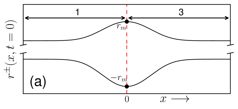
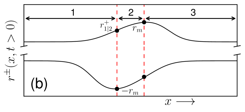
Figure 1: Sketch of the distributions $r^{\pm}(x,t)$ at time $t=0$ (a) and at finite time $t>0$ (b). In each panel the upper solid curve represents $r^{+}$ (always larger than $r_{0}$), and the lower one $r^{-}$ (always lower than $-r_{0}$). For $t>0$, $r^{+}$ ($r^{-}$) moves to the right (to the left) and regions 1 and 3 start to overlap. This leads to the configuration represented in panel (b) where a new region (labeled region 2) has appeared. The value of $r^{+}$ at the interface between regions 1 and 2 is denoted as $r_{1|2}^{+}$.

For determining the value of $W$ in each of the three regions 1, 2 and 3, we follow Ludford [9] and unfold the hodograph plane into three sheets as illustrated in Fig. 2(b).

Figure 2: (a) Behavior of the Riemann invariants in the characteristic plane at a given time $t$. The red straight line is the curve $\mathcal{C}$. The black solid line is the curve with parametric equation $(r_{+}(x,t),r_{-}(x,t))$. (b) The same curves on the four-sheeted unfolded surface. The colored regions 1, 2 and 3 are the same as the ones identified in Fig. 1. In our problem, the whole gray shaded domain above ${\cal C}$ is unreachable. A generic point $P$ of has coordinates ($\xi,\eta$) and points $A_{1}$, $B_{1}$, $A_{3}$, $B_{3}$ and $C$ lie on the initial curve $\mathcal{C}$. Points $A_{2}$ and $B_{2}$ lie on a boundary between two regions. The arrows indicate the direction of integration in Eqs. (21) and (29).

For the specific initial condition (4), the curve $\mathcal{C}$ is represented by the anti-diagonal ($r_{-}=-r_{+}$) and the points $A$ and $B$ of Eq. (21) have coordinates $A(-\eta,\eta)$ and $B(\xi,-\xi)$. Eqs. (12) with $t=0$ give

$$\left.\frac{\partial W}{\partial r_{+}}\right|_{\mathcal{C}}=\left.\frac{\partial W}{\partial r_{-}}\right|_{\mathcal{C}}=x.$$

This implies that $W$ keeps a constant value along $\mathcal{C}$. The value of this constant is immaterial, we take $W|_{\mathcal{C}}=0$ for simplicity, and Eqs. (22) then reduce to

$$U=\frac{x}{2}R(r,-r;\xi,\eta),\;\;V=-\frac{x}{2}R(r,-r;\xi,\eta).$$ (27)

We thus obtain from (21) $W=\int_{-\eta}^{\xi}xR\upd r$ which gives in regions 1 and 3 the explicit expressions

$$W^{(1,3)}(\xi,\eta)=\mp\int_{-\eta}^{\xi}\overline{x}(r)R(r,-r;\xi,\eta)\upd r,$$ (28)

where the sign $-$ ($+$) applies in region 1 (3). The difference in signs comes from the fact that $x=\mp\,\overline{x}(r)$ depending on if one is in region 1 or 3 [see Eq. (24)].

When $P$ is in region 2 one applies formula (21) with an integration path different from the one used in regions 1 and 3, see Fig. 2. Upon integrating by parts one obtains

$$\begin{split}W^{(2)}(P)=&\left(RW^{(1)}\right)_{B_{2}}+\left(RW^{(3)}\right)_{A_{2}}\\ &+\int_{A_{2}}^{C}\left(\frac{\partial R}{\partial r_{-}}-aR\right)_{r_{+}=r_{m}}\!\!\!\!\!\!\!\!\!W^{(3)}\,\upd r_{-}\\ &-\int_{C}^{B_{2}}\left(\frac{\partial R}{\partial r_{+}}-bR\right)_{r_{-}=-r_{m}}\!\!\!\!\!\!\!\!\!W^{(1)}\,\upd r_{+},\end{split}$$ (29)

where the coordinates of the relevant points are: $A_{2}(r_{m},\eta)$, $B_{2}(\xi,-r_{m})$ and $C(r_{m},-r_{m})$ (see Fig. 2). For small enough time of evolution, $\xi$ is close to $r_{m}$ and $\eta$ is close to $-r_{m}$, the integrand functions in Eq. (29) are then small by virtue of Eqs. (19). A simple approximation thus consists in keeping only the two first terms in the right-hand side of (29).

It now remains to determine the Riemann function $R$ for computing expression (28) of $W$ in regions 1 and 3 and completely solving the problem. One first remarks that the conditions (19) and (20) yield

$$\begin{split}&R(r_{+},\eta;\xi,\eta)=\sqrt{\frac{c(\xi-\eta)}{c(r_{+}-\eta)}}\exp\left(\int_{\xi-\eta}^{r_{+}-\eta}\!\!\!\frac{\upd r}{2\,c(r)}\right),\\ &R(\xi,r_{-};\xi,\eta)=\sqrt{\frac{c(\xi-\eta)}{c(\xi-r_{-})}}\exp\left(\int_{\xi-\eta}^{\xi-r_{-}}\!\!\!\frac{\upd r}{2\,c(r)}\right).\end{split}$$ (30)

These expressions suggest that $R$ can be sought in the form

$$R(r_{+},r_{-};\xi,\eta)={\mathscr{R}}(r_{+}-r_{-},\xi-\eta)F(r_{+},r_{-};\xi,\eta),$$ (31)

where $F(r_{+},\eta;\xi,\eta)=1=F(\xi,r_{-};\xi,\eta)$ and

$$\begin{split}{\mathscr{R}}(r_{1},r_{2})&=\sqrt{\frac{c(r_{2})}{c(r_{1})}}\,\exp\left(\int_{r_{2}}^{r_{1}}\!\frac{\upd r}{2\,c(r)}\right)\\ &=\sqrt{\frac{c(r_{2})\rho(r_{1})}{c(r_{1})\rho(r_{2})}}.\end{split}$$ (32)

The final expression in the above formula has been obtained by means of a change of variable $\rho=\rho(r)$ in the integral, where the function $\rho(r)$ is the reciprocal function of $r(\rho)$ given in (9)

$$r(\rho)=\int_{0}^{\rho}\frac{c(\rho^{\prime})\upd\rho^{\prime}}{\rho^{\prime}},$$ (33)

and $c(r)=c(\rho(r))$, so that $\upd r/c(r)=\upd\rho/\rho$.

We note here that the approximation previously used for discarding the integrated terms in the right-hand side of Eq. (29) amounts to assume that $F\simeq 1$. Similarly, in expression (28) for $W^{(1)}$ and $W^{(3)}$, since at short time $-\eta$ and $\xi$ are close, the integration variable $r$ is close to $\xi$ and one can again assume that $F\simeq 1$. That is to say, we are led to make in the whole hodograph plane the approximation

$$R(r_{+},r_{-};\xi,\eta)\simeq{\mathscr{R}}(r_{+}-r_{-},\xi-\eta).$$ (34)

We can now write the final approximate results, making the replacements $\xi\to r_{+}$, $\eta\to r_{-}$ in the above expressions, so that they can be used in Eqs. (12) and (15):

$$\begin{split}&W^{(1,3)}(r_{+},r_{-})\simeq\mp\int_{-r_{-}}^{r^{+}}\!\!\!\!\overline{x}(r)\,{\mathscr{R}}(2r,r_{+}-r_{-})\upd r,\\ &W^{(2)}(r_{+},r_{-})\simeq\,{\mathscr{R}}(r_{+}+r_{m},r_{+}-r_{-})\,W^{(1)}(r_{+},-r_{m})\\ &\phantom{W^{2}(r_{+},r_{-})}+{\mathscr{R}}(r_{m}-r_{-},r_{+}-r_{-})\,W^{(3)}(r_{m},r_{-}),\end{split}$$ (35)

where ${\mathscr{R}}$ is given by Eq. (32). Formulae (34) and (35) are the main results of the present work. It is important to stress that Eq. (32) has a universal form and can be applied to any physical system with known dependence $c(r_{+}-r_{-})$, see Eqs. (8) and (9).

4 Examples

In the case of the dynamics of a polytropic gas with $c(\rho)=\rho^{(\gamma-1)/2}$, an easy calculation gives

$${\mathscr{R}}(r_{1},r_{2})=\left(\frac{r_{1}}{r_{2}}\right)^{\beta},\quad\mbox{where}\quad\beta=\frac{3-\gamma}{2(\gamma-1)}.$$ (36)

It is worth noticing that the approximation (34) yields the exact expression of the Riemann function for a classical monoatomic gas with $\gamma=5/3$ ($\beta=1$). For other values of $\beta$ the function $F$ in (31) can be shown to obey the hypergeometric equation (see, e.g., Ref. [8]) and our approximation corresponds to the first term in its series expansion. Thus, we obtain

$$\begin{split}&W^{(1,3)}(r_{+},r_{-})\simeq\mp\left(\frac{2}{r_{+}-r_{-}}\right)^{\beta}\int_{-r_{-}}^{r_{+}}\!r^{\beta}\,\overline{x}(r)\upd r,\\ &W^{(2)}(r_{+},r_{-})\simeq\left(\frac{2}{r_{+}-r_{-}}\right)^{\beta}\\ &\phantom{W^{(2)}(r_{+},r_{-})}\times\left\{\int_{-r_{-}}^{r_{m}}\!\!\!r^{\beta}\,\overline{x}(r)\upd r+\int_{r_{+}}^{r_{m}}\!\!\!r^{\beta}\,\overline{x}(r)\upd r\right\}.\end{split}$$ (37)

For the case of “shallow water” equations with $\gamma=2$ ($\beta=1/2$) these formulae reproduce the results of Refs. [4, 5]. The approximation (37) cannot be distinguished from the exact result of Riemann’s approach for the type of initial condition considered in Ref. [4].

We now study in some details a case where the dependence of $c$ on $\rho$ is less simple than the one of Eq. (2): this is the case of a zero temperature Bose-Einstein condensate transversely confined in an atomic wave guide. For a harmonic trapping, the transverse averaged chemical potential can be represented by the interpolating formula [10]

$$\mu_{\perp}(\rho)=\hbar\omega_{\perp}\sqrt{1+4a\rho},$$ (38)

where $\omega_{\perp}$ is the angular frequency of the transverse harmonic potential, $a>0$ is the $s$-wave scattering length, and $\rho(x,t)$ is the linear density of the condensate. We note that other expressions for $\mu_{\perp}$ have also been proposed in the literature [11, 12]. Expression (38) yields the correct sound velocity $mc^{2}=\rho\,\upd\mu_{\perp}/\upd\rho$ both in the low ($a\rho\ll 1$) and in the high ($a\rho\gg 1$) density regimes. In these two limiting cases the long wave length dynamics of the system is thus correctly described by the hydrodynamic equations (2) with, in appropriate dimensionless units:

$$c^{2}(\rho)=\frac{\rho}{\sqrt{1+\rho}}\;,$$ (39)

where one has made the changes of variables $4a\rho\to\rho$, $u/u_{0}\to u$, $x/x_{0}\to x$ and $t/t_{0}\to t$, where $2mu_{0}^{2}=\hbar\omega_{\perp}$ and $t_{0}=x_{0}/u_{0}$. The length $x_{0}$ used to non-dimensionalize the dispersionless equations is a free parameter: we will chose it equal to the parameter $x_{0}$ appearing in the initial condition (25). We note here that the initial condition (25) can be realized by several means in the context of BEC physics. One can for instance suddenly switch on at $t=0$ a blue detuned focused laser beam [13]. An alternative method has been demonstrated in Ref. [14]: by monitoring the relative phase of a two species condensate, one can implement a bump (or a through) in one of the components.

In the case characterized by Eqs. (38) and (39), expressions (32) and (33) yield

$${\mathscr{R}}(r_{1},r_{2})=\left(\frac{\rho^{2}(r_{1})+\rho^{3}(r_{1})}{\rho^{2}(r_{2})+\rho^{3}(r_{2})}\right)^{1/8},$$ (40)

where $\rho(r)$ is the reciprocal function of

$$r(\rho)=2\int_{0}^{\sqrt{\rho}}\frac{\upd u}{(1+u^{2})^{1/4}}.$$ (41)

In order to evaluate $W$ it then suffices to determine $\overline{x}(r)$ by inverting the relation (23) and to compute the appropriate integrals (35). Once $W(r_{+},r_{-})$ is known in all three regions 1, 2 and 3, it is possible to compute $r_{+}(x,t)$ and $r_{-}(x,t)$, and then $\rho(x,t)$ and $u(x,t)$ as explained in Refs. [4, 5]:

• One first determines the value $r^{+}_{1|2}(t)$ reached by $r^{+}$ at the boundary between regions 1 and 2, see Fig. 1(b). This boundary corresponds to the point where $r^{-}=-r_{m}$ at time $t$. From Eqs. (12), $r^{+}_{1|2}(t)$ is thus determined by solving

  $$\frac{w_{+}^{(1)}(r^{+}_{1|2},-r_{m})-w_{-}^{(1)}(r^{+}_{1|2},-r_{m})}{v_{+}(r^{+}_{1|2},-r_{m})-v_{-}(r^{+}_{1|2},-r_{m})}+t=0\;,$$ (42)

  where $w_{+}^{(1)}=\partial W^{(1)}/\partial r^{+}$. We then know that, in region 1 at time $t$, $r^{+}$ takes all possible values between $r_{0}$ and $r^{+}_{1|2}(t)$ (cf. Figs. 1 and 2).

• One then let $r^{+}$ vary in $[r_{0},r_{m}]$. From Eqs. (12), at time $t$, the other Riemann invariant $r^{-}$ is solution of

  $$\frac{w_{+}^{(1,2)}(r^{+},r^{-})-w_{-}^{(1,2)}(r^{+},r^{-})}{v_{+}(r^{+},r^{-})-v_{-}(r^{+},r^{-})}+t=0\;,$$ (43)

  where the superscript should be (1) if $r^{+}\in[r_{0},r^{+}_{1|2}(t)]$ and (2) if $r^{+}\in[r^{+}_{1|2}(t),r_{m}]$.

• At this point, for each value of $t$ and $r^{+}$ we have determined the value of $r^{-}$. The position $x$ is then obtained by either one of Eqs. (12). So, for given $t$ and $r^{+}$ in regions 1 and 2, one has determined the values of $r^{-}$ and $x$. In region 3 we use the symmetry of the problem and write $r^{\pm}(x,t)=-r^{\mp}(-x,t)$.

The above procedure defines a mapping of the whole physical $(x,t)$ space onto the hodograph $(r^{+},r^{-})$ space. The density and velocity profiles are then obtained by means of Eqs. (5). The results are compared with numerical simulations in Fig. 3 for an initial profile (25) with $\rho_{0}=1$ and $\rho_{1}=1$. The simulations have been performed by solving numerically a generalized nonlinear Schrödinger equation of the form

$${\rm i}\psi_{t}=-\tfrac{1}{2}\psi_{xx}+2\,\psi\sqrt{1+\rho},$$ (44)

where $\rho(x,t)=|\psi|^{2}$, $u(x,t)=(\psi^{*}\psi_{x}-\psi\,\psi_{x}^{*})/(2{\rm i}\rho)$ and $\psi(x,0)=\sqrt{\rho}(x,0)$. This effective Gross-Pitaevskii equation reduces to the system (1) with the speed of sound (39) in the dispersionless limit. It yields an excitation spectrum always of Bogoliubov type, which is incorrect in the large density limit ($\rho\gg 1$). However, one can show that Eq. (44) is acceptable even in this limit provided one remains in the long wave-length, hydrodynamic regime. It is not appropriate when rapid oscillations appear in the density and velocity (if $\rho\gg 1$) such as observed in Fig. 3 for $t/t_{0}=3$. These oscillations correspond to the onset of a dispersive shock wave, which occurs at a time denoted as the wave breaking time: $t_{\rm\scriptscriptstyle WB}$. For $t>t_{\rm\scriptscriptstyle WB}$ the numerical simulations can be considered as accurately describing the physical system only when $\rho\ll 1$. But for $t>t_{\rm\scriptscriptstyle WB}$ our dispersionless approach also fails (see below): we are thus safe when comparing our results with numerical simulations at earlier times.

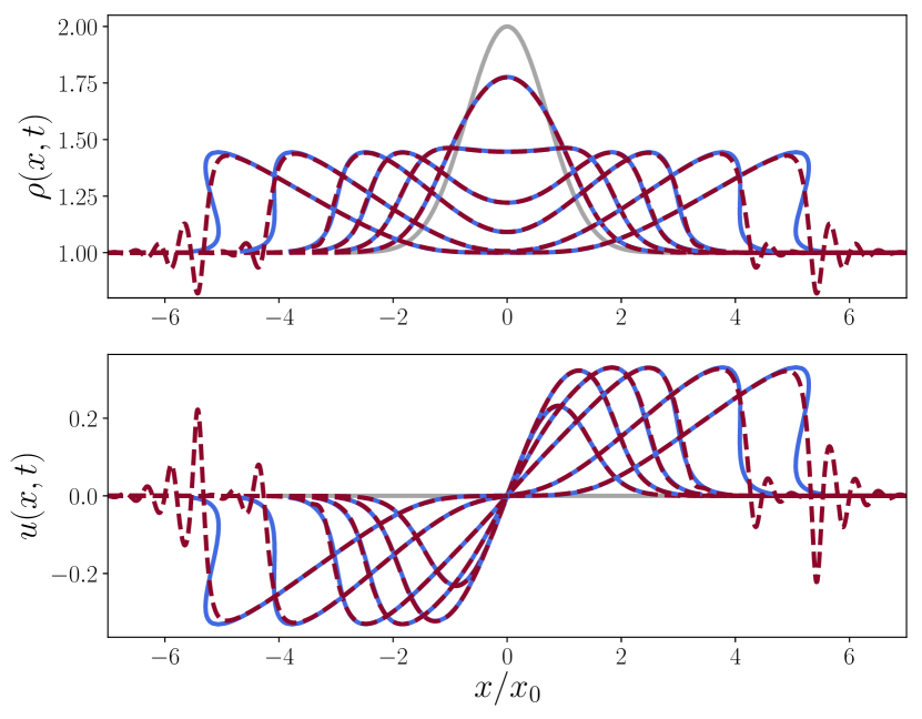
Figure 3: Density and velocity plotted as a function of $x/x_{0}$ for dimensionless times $t/t_{0}=0.5$, 1, 1.5, 2, 3 and 4 respectively. The initial conditions are given by Eqs. (4) and (25) with $\rho_{0}=1$ and $\rho_{1}=1$, they are represented by the gray solid lines. The blue solid lines are the results of the hydrodynamic system (1) obtained from the approximate Riemann’s approach described in the text. The dashed lines are the results of the numerical simulations of Eq. (44).

One sees in Fig. 3 that our solution of the hydrodynamic equations (1) agrees very well with the numerical simulations of the dispersive equation (44) at short time. For larger times the profile steepens, eventually reaching a point of gradient catastrophe at time $t_{\rm\scriptscriptstyle WB}$. It is thus expected that for $t\simeq t_{\rm\scriptscriptstyle WB}$ the solution of the dispersionless system (1) departs from the numerical simulations, as seen in the figure. However, this difference is not a sign of a failure of our approximation, but it rather points to the breakdown of the hydrodynamic model (1). After $t_{\rm\scriptscriptstyle WB}$ the system (1) leads to a multi-valued solution if not corrected to account for dispersive effects, as can be seen in Fig. 3.

5 Wave breaking time

We now turn to the determination of the wave breaking time $t_{\rm\scriptscriptstyle WB}$ at which a shock is formed. After $t_{\scriptscriptstyle\rm WB}$ the system (1) has to be modified in order to account for viscous and/or dispersive effects, depending on the physical situation under consideration.

We treat the case of an initial profile roughly of the type (25): a bump over a uniform background. Wave breaking corresponds to the occurrence of a gradient catastrophe for which $\partial r_{\pm}/\partial x=\infty$. If one considers for instance the right part of the profile (region 3), from Eq. (12), this occurs at a time $t$ such that

$$t=-\frac{\partial w_{+}^{(3)}/\partial r_{+}}{1+c^{\prime}(r_{+}-r_{-})}=-\frac{\partial w^{(3)}_{+}/\partial r_{+}}{1+\left.\frac{\displaystyle\upd\ln c}{\displaystyle\upd\ln\rho}\right|_{r_{+}-r_{-}}},$$ (45)

and $t_{\rm\scriptscriptstyle WB}$ is the smallest of the times (45). It is worth noticing that this formula yields an expression for the breaking time obtained from our approximate solution of the initial value problem and in this sense it provides less general but more definite result than the upper estimate of the breaking time obtained by Lax in Ref. [15].

One can easily compute $t_{\rm\scriptscriptstyle WB}$ approximately when the point of largest gradient in $\overline{\rho}(x)$ lies in a region where $\overline{\rho}\simeq\rho_{0}$. This occurs for some specific initial distributions (such as the inverted parabola considered in Ref. [4]) or when the initial bump is only a small perturbation of the background. In this case, it is legitimate to assume that wave breaking is reached for $r_{-}\simeq-r_{0}$ and that

$$r_{+}-r_{-}\simeq\tfrac{1}{2}\int_{0}^{\rho}\frac{c(\rho^{\prime})}{\rho^{\prime}}\upd\rho^{\prime}+\tfrac{1}{2}\int_{0}^{\rho_{0}}\frac{c(\rho^{\prime})}{\rho^{\prime}}\upd\rho^{\prime}.$$ (46)

Eqs. (15) and (35) then lead to $w_{+}^{(3)}\simeq\overline{x}(r_{+})$ and (45) becomes

$$t\simeq-\frac{2}{1+\left.\frac{\displaystyle\upd\ln c}{\displaystyle\upd\ln\rho}\right|_{\overline{\rho}}}\times\frac{\overline{\rho}}{c(\overline{\rho})\;\frac{\displaystyle\upd\overline{\rho}}{\displaystyle\upd x}}\;,$$ (47)

where $\overline{\rho}$ stands for $\overline{\rho}(\overline{x}(r^{+}))$. Within our hypothesis, it is legitimate to assume that the shortest of times $t$ is reached close to the point $\overline{x}(r^{+})$ for which $|\upd\overline{\rho}/\upd x|$ is maximal. We note $x^{*}$ the coordinate of this point and $\rho^{*}=\overline{\rho}(x^{*})$. One thus obtains

$$t_{\rm\scriptscriptstyle WB}\simeq\frac{2}{1+\left.\frac{\displaystyle\upd\ln c}{\displaystyle\upd\ln\rho}\right|_{\rho^{*}}}\times\frac{\rho^{*}}{c(\rho^{*})\,\cdot\,{\rm max}\left|\frac{\displaystyle\upd\overline{\rho}}{\displaystyle\upd x}\right|}\;.$$ (48)

In a “shallow water” case with $\gamma=1/2$ and for an initial profile where the bump is an inverted parabola, such as considered in Ref. [4], the above formula is exact.

For the initial profile (25), in the case where the speed of sound is given by (39), formula (48) yields

$$t_{\rm\scriptscriptstyle WB}\simeq\sqrt{\frac{e}{2}}\,\frac{8(1+\rho^{*})}{6+5\rho^{*}}\frac{x_{0}}{c(\rho^{*})}\frac{\rho^{*}}{\rho_{1}}.$$ (49)

The location $x_{\scriptscriptstyle\rm WB}$ of the wave breaking event can be obtained from (12). Within our approximation scheme, this yields, for the right part of the profile:

$$x_{\scriptscriptstyle\rm WB}\simeq x^{*}+c(\rho^{*})t_{\scriptscriptstyle\rm WB}.$$ (50)

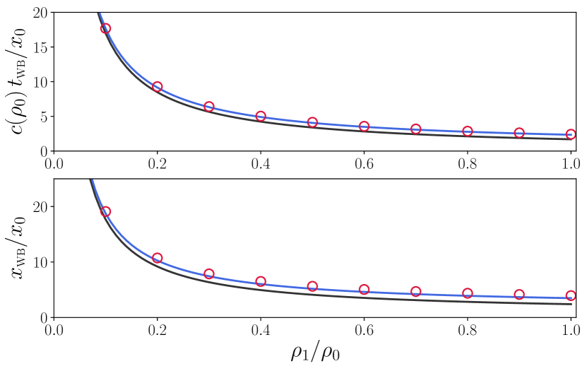
Figure 4: Wave breaking time $t_{\scriptscriptstyle\rm WB}$ and position of the wave breaking event $x_{\scriptscriptstyle\rm WB}$ for different values of $\rho_{1}/\rho_{0}$. The system considered is a quasi-1D BEC for which the speed of sound in given by (39). The initial profile is given by Eqs. (4) and (25). The blue solid lines are the approximate results (49) and (50). The red dots are the results obtained from Riemann’s approach. The black solid lines are obtained by replacing $\rho^{*}$ by $\rho_{0}$ in Eqs. (49) and (50), see the text.

These results are compared in Fig. 4 with the values determined from the Riemann approach. The overall agreement is excellent. We also note that replacing $\rho^{*}$ by $\rho_{0}$ in Eqs. (49) and (50) gives a result which is less accurate, but still quite reasonable, see Fig. 4.

6 Conclusion

We have presented an approximate method for describing the hydrodynamic evolution of a nonlinear pulse. The method is quite general and applies for any type of nonlinearity. It has been tested for cases of experimental interest in the context of nonlinear optics in Ref. [4] and here for studying the spreading of a nonlinear pulse in a guided atomic Bose-Einstein condensate. This last example is of particular interest for bench-marking the approach because the nonlinearity at hand has a non-trivial density dependence.

One could imagine to extend the present study in several directions. A possible track would be to solve the dispersionless shallow water equations [Eqs. (1) and (2) with $\gamma=2$] for more general initial conditions than discussed in the present work, as considered for instance in Refs. [16, 17] in the context of the initial stage of formation of a tsunami. Future studies could also test the present approach in the optical context for pulses propagating in a nonlinear photo-refractive material, where, up to now, no theoretical method was known for dealing with the dispersionless stage of evolution. In this context we note that the simple and accurate approximate analytic results obtained for $t_{\scriptscriptstyle\rm WB}$ and $x_{\scriptscriptstyle\rm WB}$ [Eqs. (49) and (50)] should be helpful for determining the best parameters for an experimental observation of the wave breaking phenomenon.

We finally stress that the approximate scheme presented in this work, providing an accurate account of the stage of non-dispersive propagation of a pulse, is an important and necessary step for studying the post wave breaking dynamics, and particularly the formation of dispersive shock waves in non-integrable systems.

References

• [1] \NameLandau L. D. Lifshitz E. M. \BookFluid Mechanics \PublPergamon, Oxford \Year1987
• [2] \NameForest M. G., Rosenberg C.-J., Wright III O. C. \REVIEWNonlinearity2220092287
• [3] \NameIvanov S. K. Kamchatnov A. M. \REVIEWPhys. Rev. A992019013609
• [4] \NameIsoard M., Kamchatnov A. M. Pavloff N. \REVIEWPhys. Rev. A992019053819
• [5] \NameIsoard M., Kamchatnov A. M. Pavloff N. \BookCompte-rendus de la 22${}^{\,\rm e}$ rencontre du Non Linéaire \EditorFalcon E, Lefranc M., Pétrélis F., Pham C.-T. \PublNon-Linéaire Publications, Saint-Étienne du Rouvray \Year2019\Page33
• [6] \NameKamchatnov A. M. \BookNonlinear Periodic Waves and Their Modulations—An Introductory Course \PublWorld Scientific, Singapore \Year2000
• [7] \NameTsarev S. P. \REVIEWMath. USSR Izv371991397 10.1070/IM1991v037n02ABEH002069
• [8] \NameSommerfeld A. \BookPartial Differential Equations in Physics \PublAcademic Press, New York \Year1964.
• [9] \NameLudford G. S. S. \REVIEWProc. Camb. Phil. Soc.481952499
• [10] \NameGerbier F. \REVIEWEurophys. Lett.662004771
• [11] \NameSalasnich L., Parola A. Reatto L. \REVIEWPhys. Rev. A652002043614
• [12] \NameKamchatnov A. M. Shchesnovich V. S. \REVIEWPhys. Rev. A702004023604
• [13] \NameAndrews M. R., Kurn D. M., Miesner H.-J., Durfee D. S., Townsend C. G., Inouye S. Ketterle W. \REVIEWPhys. Rev. Lett.791998553
• [14] \NameHall D. S., Matthews M. R., Wieman C. E. Cornell E. A. \REVIEWPhys. Rev. Lett.8119981543
• [15] \NameLax P. D. \REVIEWJ. Math. Phys.51964611
• [16] \NamePelinovsky E. N. A. A. Rodin A. A. \REVIEWIzv. Atmos. Ocean. Phys.492013548
• [17] \NameRodin A. A., Rodina N. A., Kurkin A. A. Pelinovsky E. N. \REVIEWIzv. Atmos. Ocean. Phys.552019374