Probabilistic motional averaging

Abstract

In a continuous measurement scheme a spin-1/2 particle can be measured and simultaneously driven by an external resonant signal. When the driving is weak, it does not prevent the particle wave-function from collapsing and a detector randomly outputs two responses corresponding to the states of the particle. In contrast, when driving is strong, the detector returns a single response corresponding to the mean of the two single-state responses. This situation is similar to a motional averaging, observed in nuclear magnetic resonance spectroscopy. We study such quantum system, being periodically driven and probed, which consists of a qubit coupled to a quantum resonator. It is demonstrated that the transmission through the resonator is defined by the interplay between driving strength, qubit dissipation, and resonator linewidth. We demonstrate that our experimental results are in good agreement with numerical and analytical calculations.

I Introduction

Circuit quantum electrodynamics studies scalable solid-state quantum systems, behaving analogous to the interacting light and matter, with superconducting qubits playing the role of artificial atoms. At this point, a number of quantum phenomena, known from atomic and optical physics, have been demonstrated in solid-state systems, such as lasing and cooling of the electromagnetic field in a resonator Astafiev et al. (2007); Ashhab et al. (2009a); Grajcar et al. (2008); Nori (2008); Hauss et al. (2008); You et al. (2008) and Mollow triplet Zhou et al. (2008); Astafiev et al. (2010); Greenberg and Sultanov (2017); Abdumalikov et al. (2011). Another phenomenon, called the motional averaging effect, which originated from nuclear magnetic resonance spectroscopy Abragam (1986), has been also recently demonstrated with a superconducting qubit Li et al. (2013). In that experiment, the qubit was driven by stochastic pulses. At the same time, a two tone spectroscopy was performed, which showed that the two spectroscopic lines (corresponding to two different states) are converted to a single broadened line for slow jumping rates, showing an increase of the average jumping rate Li et al. (2013); Abragam (1986). Different aspects of the motional averaging were studied recently, such as classical analogies Ivakhnenko et al. (2018), weighted averaging Ono et al. (2019) and related studies (see Refs. Kono et al. (2017); Pan et al. (2017)).

Reminiscent of motional averaging can be observed in a qubit-resonator system where, instead of a noisy signal, the qubit is driven by a periodic pump, with frequency $\omega_{\mathrm{d}}$ and amplitude $\mathrm{\Omega}$. The resonator which is dispersively coupled to the qubit, can be probed through its own driving term with frequency $\omega$. The resulting transmission through the resonator exhibits two resonant lines for the weak qubit driving corresponding to the qubit states and a single line in between for when the qubit driving is increased, see Fig. 1. This was demonstrated recently for a transmon-based system and termed quantum rifling Szombati et al. due to the lack of measurement back-action on the qubit from the driven resonator to the strongly driven qubit; see also Refs. Ashhab et al. (2009b, c). In this paper, we do not study measurement back-action but focus on the motional averaging picture for the resonator line and obtain simplified analytical expressions for resonator transmission.

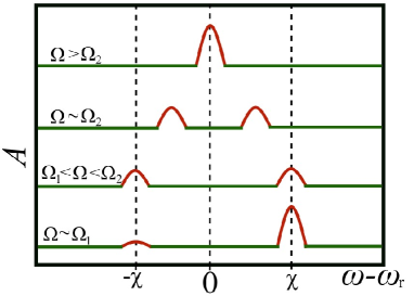
Figure 1: Schematic of probabilistic motional averaging. If driven by a periodic signal, qubit’s response (the resonator transmission amplitude $A$) is defined by the energy-level occupation probabilities. The height of the two peaks at $\mathrm{\Omega}\sim\mathrm{\Omega}_{1}$ is defined by the upper-level occupation probability and their position is defined by the dispersive shift $\chi$. With increasing $\mathrm{\Omega}$, the two peaks, first, become of equal height and then merge into one, which we term as a probabilistic motional averaging. The characteristic frequency $\mathrm{\Omega}_{1}$ denotes when the upper-level occupation probability becomes significant and $\mathrm{\Omega}_{2}$ is in-between the two regimes: (i) when the peaks are at $\omega-\omega_{\mathrm{r}}=\pm\chi$ and (ii) when they merge into one, at $\omega=\omega_{\mathrm{r}}$.

Interaction of a quantum system with a quantized electromagnetic field is considered in the frame of the quantum Rabi model Schleich (2001); Scully and Zubairy (1997); Gu et al. (2017); Kockum and Nori (2019); Pirkkalainen et al. (2014); Silveri et al. (2013); Saiko et al. (2012). In the situation where the coupling strength $\mathrm{g}$ between the two-level system and the electromagnetic field is much smaller than the difference between the qubit $\omega_{\mathrm{q}}$ and resonator $\omega_{\mathrm{r}}$ frequencies, $\left|\omega_{\mathrm{q}}-\omega_{\mathrm{r}}\right|>\mathrm{g}$, this is known as the Jaynes-Cummings model Scully and Zubairy (1997); Zagoskin (2011); Wendin (2017); Shevchenko (2019); Saiko et al. (2014).

Experiments are largely described by the semi-classical approximation, e.g. Refs. Astafiev et al. (2007); You et al. (2007a); Grajcar et al. (2008); Hauss et al. (2008); Scarlino et al. (2018); Silveri et al. (2015); Ian et al. (2010); Oelsner et al. (2013); Shevchenko et al. (2014); Karpov et al. (2016); Oelsner et al. ; Chang et al. (2019), when a chain of equations is restrained by keeping only the first-order correlators. To describe time-evolution experiments, a semi-quantum approach is more correct Szombati et al. ; Bianchetti et al. (2009); André et al. (2009); comparison of the two approaches can be found e.g. in Ref. Shevchenko and Karpov (2018). Note that in practice, to get a spectrum of a non-linear level structure of the system, one should apply two signals, to drive the system and a weak probe tone, which is known as a two-tone spectroscopy Saiko et al. (2016); Oelsner et al. ; Kohler (2018).

In this paper, we study measurement of a two-level system in the Rabi model, which is coupled to a coplanar-waveguide resonator as a cavity. The response of the system is calculated using the master equation for the density operator both numerically in the semi-quantum approximation and analytically in the semi-classical approximation. Varying the driving amplitude, we observe two different regimes, analogously to Ref. Szombati et al. : (i) weak-driving regime and (ii) strong-driving regime. In the first one, the weak-driving regime (i), both the ground and excited qubit states are monitored, displaying their probabilistic energy-level occupations. And when the power of driving is strong enough, in the strong-driving regime (ii), the spectral lines converge into a peak centered at the bare cavity and qubit transition frequencies. We note that the transition between these regimes can also be referred to as the driven quantum-to-classical transition Pietikäinen et al. (2018, 2017, 2019).

II Model

We study a two-level system which is coupled to a cavity. The system is driven by two signals: the high-amplitude driving tone with the frequency $\omega_{\mathrm{d}}$ and the low-amplitude probe tone with the frequency $\omega$. The qubit-resonator system we consider in the circuit-QED realization; specifically, it can be the driven transmon-resonator system You et al. (2007b); Koch et al. (2007); Bianchetti et al. (2009); Bishop et al. (2009), which is described by the Jaynes-Cummings Hamiltonian Schleich (2001) in the two-level approximation:

$$H = \hbar\omega_{\mathrm{r}}a^{{\dagger}}a+\hbar\frac{\omega_{\mathrm{q}}}{2}\sigma_{z}+\hbar\mathrm{g}\left(\sigma_{-}a^{{\dagger}}+\sigma_{+}a\right)+$$

$$+\hbar\xi\left(a^{{\dagger}}e^{-i\omega t}+ae^{i\omega t}\right)+\hbar\mathrm{\Omega}\left(\sigma_{+}e^{-i\omega_{\mathrm{d}}t}+\sigma_{-}e^{i\omega_{\mathrm{d}}t}\right).$$

Here, $\hbar\omega_{\mathrm{q}}$ is the transition energy between qubit states; $\sigma_{i}$ and $\sigma_{\pm}=\left(\sigma_{x}\pm i\sigma_{y}\right)/2$ are Pauli operators; the resonator has the quantized fundamental mode with frequency $\omega_{\mathrm{r}}$; $a^{{\dagger}}(a)$ is the creation (annihilation) operator of a single excitation in the resonator; the coupling strength between the two-level system and the resonator is defined by $\hbar\mathrm{g}$; the probe and drive amplitudes are described by values $\xi$ and $\mathrm{\Omega}$, respectively. Note that the transmon-resonator coupling constant $\mathrm{g}$ relates to the bare coupling $\mathrm{g}_{0}$ as $\mathrm{g}=\mathrm{g}_{0}\sqrt{E_{\mathrm{c}}/\left|\mathrm{\Delta}-E_{\mathrm{c}}\right|}$ with the detuning $\mathrm{\Delta}=\hbar\left(\omega_{\mathrm{q}}-\omega_{\mathrm{r}}\right)$ and the qubit charging energy $E_{\mathrm{c}}$, where this renormalization is due to the virtual transitions through the upper transmon states. In the experiments, e.g. Refs. Bishop et al. (2009); Bianchetti et al. (2009); Oelsner et al. (2013), the measured value is the normalized transmission amplitude $A$. This is related to the photon field $\left\langle a\right\rangle$ in the cavity Bianchetti et al. (2009); Bishop et al. (2009); Macha et al. (2014); Rakhmanov et al. (2008), $A=2V_{0}\left|\left\langle a\right\rangle\right|$, where $V_{0}$ is a voltage related to the gain of the experimental amplification chain Bishop et al. (2009) and it is defined as Bianchetti et al. (2009) $V_{0}^{2}=Z\hbar\omega_{\mathrm{r}}\varkappa/4$ with $Z$ standing for the transmission-line impedance.

III Semi-classical approach: analytical solution

To quantitatively describe the system, we first take the master equation in the form of Eq. (5) from Ref. Bianchetti et al. (2009). This includes the resonator relaxation rate $\kappa$ and qubit relaxation and pure dephasing rates, $\Gamma_{1}$ and $\Gamma_{2}=\Gamma_{\phi}+\Gamma_{1}/2$. While the equations can be numerically solved in their available form, it is more illustrative to study analytical expressions first. For this purpose, we consider the steady-state solution in the so-called semi-classical approximation, where all correlators are assumed to factorize, $\!\left\langle a^{{\dagger}}\sigma\right\rangle\approx\!\left\langle a^{{\dagger}}\right\rangle\!\left\langle\sigma\right\rangle$, etc. Shevchenko and Karpov (2018) Then from the Lindblad equation, we obtain the non-linear equations for $\left\langle a\right\rangle$, $\left\langle\sigma\right\rangle$, and $\left\langle\sigma_{z}\right\rangle$. These can be rewritten for $n=\left|\left\langle a\right\rangle\right|^{2}$ and $\left\langle\sigma_{z}\right\rangle=2P_{+}-1$, with $P_{+}$ standing for the qubit upper-level occupation probability, as follows

$$n=\left|\left\langle a\right\rangle\right|^{2}=\frac{\xi^{2}}{\left[\chi\left(2P_{+}-1\right)+\delta\omega_{\mathrm{r}}\right]^{2}+\kappa^{2}},$$ (2)

$$P_{+}=\frac{1}{2}\frac{\mathrm{\Omega}^{2}}{\mathrm{\Omega}^{2}+\mathrm{\Omega}_{1}^{2}(n)},$$ (3)

$$\mathrm{\Omega}_{1}^{2}(n)=\frac{4}{T_{1}T_{2}}+4\frac{T_{2}}{T_{1}}\left(\delta\omega_{\mathrm{q}}+2\chi n\right)^{2}.$$ (4)

Here $\delta\omega_{\mathrm{r}}=\omega_{\mathrm{r}}-\omega$, $\delta\omega_{\mathrm{q}}=\omega_{\mathrm{q}}-\omega_{\mathrm{d}}$, $\chi=\mathrm{g}^{2}/\mathrm{\Delta}$ describes the dispersive shift, and $\mathrm{\Omega}_{1}$ can be interpreted from Eq. (3), as the characteristic driving amplitude $\mathrm{\Omega}$, at which the excited qubit level becomes significantly occupied. In particular, at resonance ($\delta\omega_{\mathrm{q}}=0$) in the linear approximation (neglecting the term with $n^{2}$), we have the characteristic driving amplitude as in Ref. Bishop et al. (2009): $\mathrm{\Omega}_{1}=2\left(T_{1}T_{2}\right)^{-1/2}$. In general case, the characteristic driving amplitude $\mathrm{\Omega}_{1}$ depends on the measurement amplitude $\xi$ and is defined by Eq. (4) together with Eqs. (2) and (3).

IV Semi-quantum approach: numerical solution

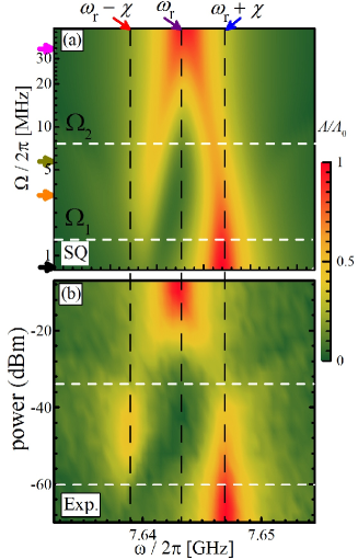
Figure 2: Regimes for the driven and probed qubit and characteristic driving amplitudes $\mathrm{\Omega}_{1}$ and $\mathrm{\Omega}_{2}$. (a) Normalized transmission amplitude $A$ as a function of the probe frequency $\omega$ and driving amplitude $\mathrm{\Omega}$. The picture is a result of the steady-state solution of Maxwell-Bloch equations (6). Horizontal colour arrows show position of the cuts, presented in the next figure. (b) Respective experimental measurement.

The system Hamiltonian (II) can be rewritten in a more illustrative form for large detuning $\mathrm{\Delta}$ between a transmon qubit (in the two-level approximation) and a resonator mode, $\mathrm{\Delta}\equiv\hbar\left(\omega_{\mathrm{q}}-\omega_{\mathrm{r}}\right)\gg\mathrm{g}$,

$$H^{\prime} = \hbar(\delta\omega_{\mathrm{r}}+\chi\sigma_{z})a^{{\dagger}}a+\hbar\frac{\delta\omega_{\mathrm{q-d}}+\chi}{2}\sigma_{z}+$$ (5)

$$+\hbar\xi(a^{\dagger}+a)+\hbar\frac{\mathrm{\Omega}}{2}(\sigma+\sigma^{\dagger}),$$

where $\delta\omega_{\mathrm{q-d}}=\omega_{\mathrm{q}}-\omega_{\mathrm{d}}$ and $\delta\omega_{\mathrm{q-r}}=\omega_{\mathrm{r}}-\omega$. It is reasonable to describe the system in the dispersive approximation of the Jaynes-Cummings Hamiltonian, as in Refs. Koch et al. (2007); Bianchetti et al. (2009); Oelsner et al. (2010). Then, following Refs. Bianchetti et al. (2009); André et al. (2009); Shevchenko and Karpov (2018), we obtain equations in the so-called semi-quantum model, where one assumes factoring of higher order terms and keeping only the second order correlators as the following: $\langle a^{\dagger}a\sigma_{i}\rangle\thickapprox\langle a^{\dagger}a\rangle\langle\sigma_{i}\rangle$ and $\langle a^{\dagger}aa\sigma_{i}\rangle\thickapprox\langle a^{\dagger}a\rangle\langle a\sigma_{i}\rangle$. This allows truncating the infinite series of equations. From the Lindblad equation, for the expectation values of the operators $\langle\sigma_{i}\rangle$ $(i=x,y,z)$ and the resonator field operators $\left\langle a\right\rangle,$ $\langle a\sigma_{i}\rangle,$ and $\langle a^{\dagger}a\rangle$ we obtain the system of equations, known as the Maxwell-Bloch equations:

$$\frac{d}{dt}\langle\sigma_{z}\rangle\! = \!\mathrm{\Omega}\langle\sigma_{y}\rangle-\Gamma_{1}\left(1+\frac{\langle\sigma_{z}\rangle}{z_{0}}\right),$$ (6a)

$$\frac{d}{dt}\langle\sigma_{x}\rangle\! = \!-\!\left(2\chi\!\left\langle a^{\dagger}a\right\rangle\!+\!\delta\omega_{\mathrm{q-d}}+\!\chi\right)\!\langle\sigma_{y}\rangle-\Gamma_{2}\!\frac{\langle\sigma_{x}\rangle}{z_{0}}\!,$$ (6b)

$$\frac{d}{dt}\langle\sigma_{y}\rangle\! = \!\left(2\chi\left\langle a^{\dagger}a\right\rangle+\delta\omega_{\mathrm{q-d}}+\chi\right)\langle\sigma_{x}\rangle-$$

$$-\Gamma_{2}\frac{\langle\sigma_{y}\rangle}{z_{0}}-\mathrm{\Omega}\langle\sigma_{z}\rangle,$$

$$\frac{d}{dt}\langle a\rangle\! = \!-i\left(\delta\omega_{\mathrm{r}}\langle a\rangle+\chi\langle a\sigma_{z}\rangle+\xi\right)-\kappa\langle a\rangle,$$ (6d)

$$\frac{d}{dt}\langle a^{\dagger}a\rangle\! = \!-2\xi\text{\thinspace Im\thinspace}\langle a\rangle+2\kappa\left(N_{\mathrm{th}}-\langle a^{\dagger}a\rangle\right),$$ (6e)

$$\frac{d}{dt}\langle a\sigma_{z}\rangle\! = \!-i\left(\delta\omega_{\mathrm{r}}\left\langle a\sigma_{z}\right\rangle+\chi\langle a\rangle+\xi\langle\sigma_{z}\rangle\right)+$$

$$+\mathrm{\Omega}\langle a\sigma_{y}\rangle-\Gamma_{1}\left\langle a\right\rangle-\left(\frac{\Gamma_{1}}{z_{0}}+\kappa\right)\langle a\sigma_{z}\rangle,$$

$$\frac{d}{dt}\langle a\sigma_{x}\rangle\! = \!-i\delta\omega_{\mathrm{r}}\left\langle a\sigma_{x}\right\rangle-\left(\frac{\Gamma_{2}}{z_{0}}+\kappa\right)\langle a\sigma_{x}\rangle-$$

$$-\left(\delta\omega_{\mathrm{q-d}}+2\chi\left(\langle a^{\dagger}a\rangle+1\right)\right)\langle a\sigma_{y}\rangle-i\xi\langle\sigma_{x}\rangle,$$

$$\frac{d}{dt}\langle a\sigma_{y}\rangle\! = \!-i\delta\omega_{\mathrm{r}}\left\langle a\sigma_{y}\right\rangle-\left(\frac{\Gamma_{2}}{z_{0}}+\kappa\right)\langle a\sigma_{y}\rangle-$$

$$-i\xi\langle\sigma_{y}\rangle-\mathrm{\Omega}\langle a\sigma_{z}\rangle+$$

$$+\left(\delta\omega_{\mathrm{q-d}}+2\chi\left(\langle a^{\dagger}a\rangle+1\right)\right)\langle a\sigma_{x}\rangle.$$

We have numerically solved the system of equations (6) and the results are presented in Figs. 2-4, where the normalized transmission amplitude is plotted as a function of the driving power and probing frequency. For calculations we take the following parameters, close to the ones of Ref. Szombati et al. :

$$\frac{\omega_{\mathrm{r}}}{2\pi} = 7.643~{}\text{GHz, \ \ }\frac{\omega_{\mathrm{q}}}{2\pi}=6.440~{}\text{GHz, \ \ }\frac{\chi}{2\pi}=4.1~{}\text{MHz},$$

$$T_{1} = 1.55~{}\mu\text{s, \ \ }T_{2}=2.65~{}\mu\text{s, \ \ }\ \kappa/2\pi=1~{}\text{MHz.}$$ (7)

V Experiment

Our sample consists of a transmon qubit (named Qubit 2 in Ref. Szombati et al. ) with a transition frequency between its ground and first excited states $\omega_{\mathrm{q}}/(2\pi)=6.44$ GHz coupled to a superconducting co-planar waveguide resonator with resonance frequency $\omega_{\mathrm{r}}/(2\pi)=7.643$ GHz. The qubit state can be controlled by applying a coherent drive tone with frequency $\omega_{\mathrm{d}}\simeq\omega_{\mathrm{q}}$ through a separate charge line. The interaction between the qubit and the resonator results in a shift of the resonator frequency dependent on the qubit state. This dispersive shift of $\chi/(2\pi)=4.1$ MHz allows us to perform the read out of the qubit state by applying a probe tone to the resonator at frequency $\omega_{\mathrm{p}}\simeq\omega_{\mathrm{r}}$ and by subsequent detection of the transmitted signal with a standard heterodyne detection scheme (see Ref. Szombati et al. ).

VI Results

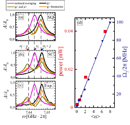
Figure 3: Shift of the resonance lines. Numerical semi-quantum (a) and analytical semi-classical (b) dependencies of the normalized transmission amplitude $A$ on the probing frequency for several values of driving power $\mathrm{\Omega}\,$, shown by the arrows in Fig. 2. Solid lines relate to regime (i) with two qubit lines and the dashed lines are for the regime (ii) with one motional-averaged line. (c) Respective experimental measurement. (d) Characteristic driving amplitude $\mathrm{\Omega}_{2}$ as a function of the photon number $\left\langle n\right\rangle$; right scale is for the theoretical points ($\mathrm{\Omega}_{2}$ in MHz) and left scale is for the experimental points (power in mW); the agreement between the data here could be used for the calibration of the power.

Numerical and analytical results of the previous two sections together with the experimental observations are presented in Figs. 2-4. Namely, in Fig. 2(a) we plot the transmission amplitude $A$, normalized to its maximal value $A_{0}$, as a function of the probe frequency $\omega$ and driving amplitude $\mathrm{\Omega}$, which is calculated using the equations and parameters from the previous section, Eqs. (6-7). Several horizontal cuts of Fig. 2(a) are presented as Fig. 2(a-c), which is the transmission plotted as a function of the probe frequency $\omega$ for several values of the drive amplitude $\mathrm{\Omega}$ (see explanations below).

In Fig. 2(a) we can observe two different regimes. Let us now analyze these regimes in more detail, since these present the main result of our work here.

(i) $\mathrm{\Omega}\ll\mathrm{\Omega}_{2}$. This can be called the “fast-measurements” regime, or equivalently weak-driving regime, or “quantum” regime. This is because the two qubit states are visualized with the position of the respective resonances at $\delta\omega=\pm\chi$. So, in this regime both ground and excited qubit states are monitored, with respective probabilities. Namely, with increasing the driving amplitude $\mathrm{\Omega}$, the probability of finding the qubit in the excited state increases, left line in Fig. 2(a), while the probability of the ground state (right resonance line) decreases. See also about this, e.g., in Ref. Reagor et al. (2016).

(ii) $\mathrm{\Omega}\gg\mathrm{\Omega}_{2}$. This can be called the “slow-measurements” regime, or equivalently strong-driving regime, or “classical” regime. This corresponds to no frequency shift, with qubit states equally populated, which thus can also be referred to as a “motional averaging”. Similar transitions from a “quantum” to “classical” regime was observed in Refs. Fink et al. (2010); Li et al. (2013); Pietikäinen et al. (2017, 2018); Szombati et al. .

Figure 3(d) shows the dependence of the characteristic driving amplitude $\mathrm{\Omega}_{2}$, which separates regimes (i) and (ii), as a function of photon numbers obtained from our numerical solution as well as the experimental points. The theoretical points were calculated for the probe amplitudes $\xi$ from $0.01\kappa$ to $2\kappa$. The experimental points were taken from Fig. S4 of Ref. Szombati et al. .

Let us now consider interpretation of the above results analytically, for the two respective regimes.

Regime (i). This is not described directly by the stationary solution. To describe this regime we note that in this case the qubit is found either in the ground state with the probability $P_{-}$ or in the excited state with the probability $P_{+}$. Then the measured normalized transmission amplitude can be calculated as following

$$A=P_{-}A_{-}+P_{+}A_{+}$$ (8)

with the partial values $A_{\pm}$ given by Eq. (2):

$$A_{\pm}=\frac{\xi}{\sqrt{\left[\pm\chi+\delta\omega_{\mathrm{r}}\right]^{2}+\kappa^{2}}}.$$ (9)

With these formulas we plot the solid lines in Fig. 3(b).

Regime (ii). Under the strong resonant driving, the qubit levels are equally populated and then Eq. (2) with $P_{+}=1/2$ yields

$$A=\frac{\xi}{\sqrt{\delta\omega_{\mathrm{r}}^{2}+\kappa^{2}}}\text{.}$$ (10)

With this formula we plot the magenta solid line in Fig. 3(a).

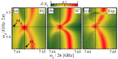
Figure 4: The resonant transmission shift. Analytical (a) and semi-quantum (b) dependencies of the normalized transmission amplitude $A$ on the probe frequency $\omega$ and the drive frequency $\omega_{\mathrm{d}}$. (c) Respective experimental measurement.

Finally we describe both the qubit and resonator frequency shifts. For this, we make use of Eq. (8) with the partial transmission amplitudes $A_{\pm}$ defined by the respective probabilities, rather than assuming them equal to $0$ or $1$ as in Eq. (9), as following

$$A_{\pm}=\frac{\xi}{\sqrt{\left[\chi\left(1-2P_{\pm}\right)+\delta\omega_{\mathrm{r}}\right]^{2}+\kappa^{2}}}.$$ (11)

With this analytical formulas we plot Fig. 4(b), which is remarkably in agreement with the numerical result in Fig. 4(a) and the experiment in Fig. 4(c).

Note that the advantage of the analytical results, presented here, is that these are transparent formulas, which capture the main physics here. Importantly, these results are confirmed by the numerical calculations, done within the semi-quantum model, and by comparison with the experiments.

VII Conclusions

We have studied the interaction between a cavity and a two-level system in the Jaynes-Cummings model with dispersive coupling under external drive. We have demonstrated that there are two different regimes. The quantum and semi-classical regimes demonstrate detection of the two energy transitions in the system, while at higher driving amplitude the two resonance lines merge into one, making a specific motional-averaging picture, defined by the qubit energy-level occupation probabilities. We believe that our analytical and numerical results are useful for deeper understanding of both experimental realizations and theoretical description of dynamical phenomena in circuit quantum electrodynamics.