Exact expressions for double descent and implicit regularization
via surrogate random design

Abstract

Double descent refers to the phase transition that is exhibited by the generalization error of unregularized learning models when varying the ratio between the number of parameters and the number of training samples. The recent success of highly over-parameterized machine learning models such as deep neural networks has motivated a theoretical analysis of the double descent phenomenon in classical models such as linear regression which can also generalize well in the over-parameterized regime. We provide the first exact non-asymptotic expressions for double descent of the minimum norm linear estimator. Our approach involves constructing a special determinantal point process which we call surrogate random design, to replace the standard i.i.d. design of the training sample. This surrogate design admits exact expressions for the mean squared error of the estimator while preserving the key properties of the standard design. We also establish an exact implicit regularization result for over-parameterized training samples. In particular, we show that, for the surrogate design, the implicit bias of the unregularized minimum norm estimator precisely corresponds to solving a ridge-regularized least squares problem on the population distribution. In our analysis we introduce a new mathematical tool of independent interest: the class of random matrices for which determinant commutes with expectation.

1 Introduction

Classical statistical learning theory asserts that to achieve generalization one must use training sample size that sufficiently exceeds the complexity of the learning model, where the latter is typically represented by the number of parameters (or some related structural parameter; see Friedman et al., 2001). In particular, this seems to suggest the conventional wisdom that one should not use models that fit the training data exactly. However, modern machine learning practice often seems to go against this intuition, using models with so many parameters that the training data can be perfectly interpolated, in which case the training error vanishes. It has been shown that models such as deep neural networks, as well as certain so-called interpolating kernels and decision trees, can generalize well in this regime. In particular, Belkin et al. (2019a) empirically demonstrated a phase transition in generalization performance of learning models which occurs at an interpolation thershold, i.e., a point where training error goes to zero (as one varies the ratio between the model complexity and the sample size). Moving away from this threshold in either direction tends to reduce the generalization error, leading to the so-called double descent curve.

To understand this surprising phenomenon, in perhaps the simplest possible setting, we study it in the context of linear or least squares regression. Consider a full rank $n\times d$ data matrix $\mathbf{X}$ and a vector $\mathbf{y}$ of responses corresponding to each of the $n$ data points (the rows of $\mathbf{X}$), where we wish to find the best linear model $\mathbf{X}\mathbf{w}\approx\mathbf{y}$, parameterized by a $d$-dimensional vector $\mathbf{w}$. The simplest example of an estimator that has been shown to exhibit the double descent phenomenon (Belkin et al., 2019c) is the Moore-Penrose estimator, $\widehat{\mathbf{w}}=\mathbf{X}^{\dagger}\mathbf{y}$: in the so-called over-determined regime, i.e., when $n>d$, it corresponds to the least squares solution, i.e., $\operatorname*{\mathop{\mathrm{argmin}}}_{\mathbf{w}}\|\mathbf{X}\mathbf{w}-\mathbf{y}\|^{2}$; and in the under-determined regime (also known as over-parameterized or interpolating), i.e., when $n<d$, it corresponds to the minimum norm solution to the linear system $\mathbf{X}\mathbf{w}=\mathbf{y}$. Given the ubiquity of linear regression and the Moore-Penrose solution, e.g., in kernel-based machine learning, studying the performance of this estimator can shed some light on the effects of over-parameterization/interpolation in machine learning more generally. Of particular interest are results that are exact (i.e., not upper/lower bounds) and non-asymptotic (i.e., for large but still finite $n$ and $d$).

We build on methods from Randomized Numerical Linear Algebra (RandNLA) in order to obtain exact non-asymptotic expressions for the mean squared error (MSE) of the Moore-Penrose estimator (see Theorem 1). This provides a precise characterization of the double descent phenomenon for the linear regression problem. In obtaining these results, we are able to provide precise formulas for the implicit regularization induced by minimum norm solutions of under-determined training samples, relating it to classical ridge regularization (see Theorem 2). To obtain our precise results, we use a somewhat non-standard random design, based on a specially chosen determinantal point process (DPP), which we term surrogate random design. DPPs are a family of non-i.i.d. sampling distributions which are typically used to induce diversity in the produced samples (Kulesza and Taskar, 2012). Our aim in using a DPP as a surrogate design is very different: namely, to make certain quantities (such as the MSE) analytically tractable, while accurately preserving the underlying properties of the original data distribution. This strategy might seem counter-intuitive since DPPs are typically found most useful when they differ from the data distribution. However, we show both theoretically (Theorem 3) and empirically (Section 5), that for many commonly studied data distributions, such as multivariate Gaussians, our DPP-based surrogate design accurately preserves the key properties of the standard i.i.d. design (such as the MSE), and even matches it exactly in the high-dimensional asymptotic limit. In our analysis of the surrogate design, we introduce the concept of determinant preserving random matrices (Section 4), a class of random matrices for which determinant commutes with expectation, which should be of independent interest.

1.1 Main results: double descent and implicit regularization

As the performance metric in our analysis, we use the mean squared error (MSE), defined as $\mathrm{MSE}[\widehat{\mathbf{w}}]=\mathbb{E}\big{[}\|\widehat{\mathbf{w}}-\mathbf{w}^{*}\|^{2}\big{]}$, where $\mathbf{w}^{*}$ is a fixed underlying linear model of the responses. In analyzing the MSE, we make the following standard assumption that the response noise is homoscedastic.

Assumption 1 (Homoscedastic noise).

The noise $\xi=y(\mathbf{x})-\mathbf{x}^{\scriptscriptstyle{\top}}\mathbf{w}^{*}$ has mean $0$ and variance $\sigma^{2}$.

Our main result provides an exact expression for the MSE of the Moore-Penrose estimator under our surrogate design denoted ${\bar{\mathbf{X}}}\sim S_{\mu}^{n}$, where $\mu$ is the $d$-variate distribution of the row vector $\mathbf{x}^{\scriptscriptstyle{\top}}$ and $n$ is the sample size. This surrogate is used in place of the standard $n\times d$ random design $\mathbf{X}\sim\mu^{n}$, where $n$ data points (the rows of $\mathbf{X}$) are sampled independently from $\mu$. We form the surrogate by constructing a determinantal point process with $\mu$ as the background measure, so that $S_{\mu}^{n}(\mathbf{X})\propto\mathrm{pdet}(\mathbf{X}\mathbf{X}^{\scriptscriptstyle{\top}})\mu(\mathbf{X})$, where $\mathrm{pdet}(\cdot)$ denotes the pseudo-determinant (details in Section 3). Unlike for the standard design, our MSE formula is fully expressible as a function of the covariance matrix $\mathbf{\Sigma}_{\mu}=\mathbb{E}_{\mu}[\mathbf{x}\mathbf{x}^{\scriptscriptstyle{\top}}]$. To state our main result, we need an additional minor assumption on $\mu$ which is satisfied by most standard continuous distributions (e.g., multivariate Gaussians).

Assumption 2 (General position).

For $1\leq n\leq d$, if $\mathbf{X}\sim\mu^{n}$, then $\mathrm{rank}(\mathbf{X})=n$ almost surely.

Under Assumptions 1 and 2, we can establish our first main result, stated as the following theorem, where we use $\mathbf{X}^{\dagger}$ to denote the Moore-Penrose inverse of $\mathbf{X}$.

Theorem 1 (Exact non-asymptotic MSE).

If the response noise is homoscedastic (Assumption 1) and $\mu$ is in general position (Assumption 2), then for ${\bar{\mathbf{X}}}\sim S_{\mu}^{n}$ (Definition 3) and ${\bar{y}}_{i}=y(\bar{\mathbf{x}}_{i})$,

$${\mathrm{MSE}\big{[}{\bar{\mathbf{X}}}^{\dagger}\bar{\mathbf{y}}\big{]}}=\begin{cases}\sigma^{2}\,\mathrm{tr}\big{(}(\mathbf{\Sigma}_{\mu}+\lambda_{n}\mathbf{I})^{-1}\big{)}\cdot\frac{1-\alpha_{n}}{d-n}\ +\ \frac{\mathbf{w}^{*{\scriptscriptstyle{\top}}}(\mathbf{\Sigma}_{\mu}+\lambda_{n}\mathbf{I})^{-1}\mathbf{w}^{*}}{\mathrm{tr}((\mathbf{\Sigma}_{\mu}+\lambda_{n}\mathbf{I})^{-1})}\cdot(d-n),&\text{for }n<d,\\ \sigma^{2}\,\mathrm{tr}(\mathbf{\Sigma}_{\mu}^{-1}),&\text{for }n=d,\\ \sigma^{2}\,\mathrm{tr}(\mathbf{\Sigma}_{\mu}^{-1})\cdot\frac{1-\beta_{n}}{n-d},&\text{for }n>d,\end{cases}$$

with $\lambda_{n}\geq 0$ defined by $n=\mathrm{tr}(\mathbf{\Sigma}_{\mu}(\mathbf{\Sigma}_{\mu}+\lambda_{n}\mathbf{I})^{-1})$,  $\alpha_{n}=\det(\mathbf{\Sigma}_{\mu}(\mathbf{\Sigma}_{\mu}+\lambda_{n}\mathbf{I})^{-1})$ and $\beta_{n}=\mathrm{e}^{d-n}$.

Definition 1.

We will use $\mathcal{M}=\mathcal{M}(\mathbf{\Sigma}_{\mu},\mathbf{w}^{*},\sigma^{2},n)$ to denote the above expressions for ${\mathrm{MSE}\big{[}{\bar{\mathbf{X}}}^{\dagger}\bar{\mathbf{y}}\big{]}}$.

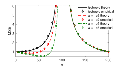
(a) Surrogate MSE expressions (Theorem 1) closely match numerical estimates even for non-isotropic features. Eigenvalue decay leads to a steeper descent curve in the under-determined regime ($n<d$).

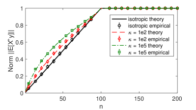
(b) The mean of the estimator $\mathbf{X}^{\dagger}\mathbf{y}$ exhibits shrinkage which closely matches the shrinkage of a ridge-regularized least squares optimum (theory lines), as characterized by Theorem 2.

Figure 1: Illustration of the main results for $d=100$ and $\mu=\mathcal{N}(\mathbf{0},\mathbf{\Sigma})$ where $\mathbf{\Sigma}$ is diagonal with eigenvalues decaying exponentially and scaled so that $\mathrm{tr}(\mathbf{\Sigma}^{-1})=d$. We use our surrogate formulas to plot (a) the MSE (Theorem 1) and (b) the norm of the expectation (Theorem 2) of the Moore-Penrose estimator (theory lines), accompanied by the empirical estimates based on the standard i.i.d. design (error bars are three times the standard error of the mean). We consider three different condition numbers $\kappa$ of $\mathbf{\Sigma}$, with isotropic corresponding to $\kappa=1$, i.e., $\mathbf{\Sigma}=\mathbf{I}$. We use $\sigma^{2}=1$ and $\mathbf{w}^{*}=\frac{1}{\sqrt{d}}\mathbf{1}$.

Proof of Theorem 1 is given in Appendix C. For illustration, we plot the MSE expressions in Figure 1a, comparing them with empirical estimates of the true MSE under the i.i.d. design for a multivariate Gaussian distribution $\mu=\mathcal{N}(\mathbf{0},\mathbf{\Sigma})$ with several different covariance matrices $\mathbf{\Sigma}$. We keep the number of features $d$ fixed to $100$ and vary the number of samples $n$, observing a double descent peak at $n=d$. We observe that our theory aligns well with the empirical estimates, whereas previously, no such theory was available except for special cases such as $\mathbf{\Sigma}=\mathbf{I}$ (more details in Theorem 3 and Section 5). The plots show that varying the spectral decay of $\mathbf{\Sigma}$ has a significant effect on the shape of the curve in the under-determined regime. We use the horizontal line to denote the MSE of the null estimator $\mathrm{MSE}[\mathbf{0}]=\|\mathbf{w}^{*}\|^{2}=1$. When the eigenvalues of $\mathbf{\Sigma}$ decay rapidly, then the Moore-Penrose estimator suffers less error than the null estimator for some values of $n<d$, and the curve exhibits a local optimum in this regime.

One important aspect of Theorem 1 comes from the relationship between $n$ and the parameter $\lambda_{n}$, which together satisfy $n=\mathrm{tr}(\mathbf{\Sigma}_{\mu}(\mathbf{\Sigma}_{\mu}+\lambda_{n}\mathbf{I})^{-1})$. This expression is precisely the classical notion of effective dimension for ridge regression regularized with $\lambda_{n}$ (Alaoui and Mahoney, 2015), and it arises here even though there is no explicit ridge regularization in the problem being considered in Theorem 1. The global solution to the ridge regression task (i.e., $\ell_{2}$-regularized least squares) with parameter $\lambda$ is defined as:

$$\operatorname*{\mathop{\mathrm{argmin}}}_{\mathbf{w}}\Big{\{}\mathbb{E}_{\mu,y}\big{[}\big{(}\mathbf{x}^{\scriptscriptstyle{\top}}\mathbf{w}-y(\mathbf{x})\big{)}^{2}\big{]}+\lambda\|\mathbf{w}\|^{2}\Big{\}}\ =\ (\mathbf{\Sigma}_{\mu}+\lambda\mathbf{I})^{-1}\mathbf{v}_{\mu,y},\quad\text{where }\mathbf{v}_{\mu,y}=\mathbb{E}_{\mu,y}[y(\mathbf{x})\,\mathbf{x}].$$

When Assumption 1 holds, then $\mathbf{v}_{\mu,y}=\mathbf{\Sigma}_{\mu}\mathbf{w}^{*}$, however ridge-regularized least squares is well-defined for much more general response models. Our second result makes a direct connection between the (expectation of the) unregularized minimum norm solution on the sample and the global ridge-regularized solution. While the under-determined regime (i.e., $n<d$) is of primary interest to us, for completeness we state this result for arbitrary values of $n$ and $d$. Note that, just like the definition of regularized least squares, this theorem applies more generally than Theorem 1, in that it does not require the responses to follow any linear model as in Assumption 1 (proof in Appendix D).

Theorem 2 (Implicit regularization of Moore-Penrose estimator).

For $\mu$ satisfying Assumption 2 and $y(\cdot)$ s.t. $\mathbf{v}_{\mu,y}=\mathbb{E}_{\mu,y}[y(\mathbf{x})\,\mathbf{x}]$ is well-defined, ${\bar{\mathbf{X}}}\sim S_{\mu}^{n}$ (Definition 3) and ${\bar{y}}_{i}=y(\bar{\mathbf{x}}_{i})$,

$$\mathbb{E}\big{[}{\bar{\mathbf{X}}}^{\dagger}\bar{\mathbf{y}}\big{]}=\begin{cases}(\mathbf{\Sigma}_{\mu}+\lambda_{n}\mathbf{I})^{-1}\mathbf{v}_{\mu,y}&\text{for }n<d,\\ \mathbf{\Sigma}_{\mu}^{-1}\mathbf{v}_{\mu,y}&\text{for }n\geq d,\end{cases}$$

where, as in Theorem 1, $\lambda_{n}$ is such that the effective dimension $\mathrm{tr}(\mathbf{\Sigma}_{\mu}(\mathbf{\Sigma}_{\mu}+\lambda_{n}\mathbf{I})^{-1})$ equals $n$.

That is, when $n<d$, the Moore-Penrose estimator (which itself is not regularized), computed on the random training sample, in expectation equals the global ridge-regularized least squares solution of the underlying regression problem. Moreover, $\lambda_{n}$, i.e., the amount of implicit $\ell_{2}$-regularization, is controlled by the degree of over-parameterization in such a way as to ensure that $n$ becomes the ridge effective dimension (a.k.a. the effective degrees of freedom).

We illustrate this result in Figure 1b, plotting the norm of the expectation of the Moore-Penrose estimator. As for the MSE, our surrogate theory aligns well with the empirical estimates for i.i.d. Gaussian designs, showing that the shrinkage of the unregularized estimator in the under-determined regime matches the implicit ridge-regularization characterized by Theorem 2. While the shrinkage is a linear function of the sample size $n$ for isotropic features (i.e., $\mathbf{\Sigma}=\mathbf{I}$), it exhibits a non-linear behavior for other spectral decays. Such implicit regularization has been studied previously (see, e.g., Mahoney and Orecchia, 2011; Mahoney, 2012); it has been observed empirically for RandNLA sampling algorithms (Ma et al., 2015); and it has also received attention more generally within the context of neural networks (Neyshabur, 2017). While our implicit regularization result is limited to the Moore-Penrose estimator, this new connection (and others, described below) between the minimum norm solution of an unregularized under-determined system and a ridge-regularized least squares solution offers a simple interpretation for the implicit regularization observed in modern machine learning architectures.

Our exact non-asymptotic expressions in Theorem 1 and our exact implicit regularization results in Theorem 2 are derived for the surrogate design, which is a non-i.i.d. distribution based on a determinantal point process. However, Figure 1 suggests that those expressions accurately describe the MSE (up to lower order terms) also under the standard i.i.d. design $\mathbf{X}\sim\mu^{n}$ when $\mu$ is a multivariate Gaussian. As a third result, we verify that the surrogate expressions for the MSE are asymptotically consistent with the MSE of an i.i.d. design, for a wide class of distributions which include multivariate Gaussians.

Theorem 3 (Asymptotic consistency of surrogate design).

Let $\mathbf{X}\in\mathbb{R}^{n\times d}$ have i.i.d. rows $\mathbf{x}_{i}^{\scriptscriptstyle{\top}}=\mathbf{z}_{i}^{\scriptscriptstyle{\top}}\mathbf{\Sigma}^{\frac{1}{2}}$ where $\mathbf{z}_{i}$ has independent zero mean and unit variance sub-Gaussian entries, and suppose that Assumptions 1 and 2 are satisfied. Furthermore, suppose that there exist $c,C,C^{*}\in\mathbb{R}_{>0}$ such that $C\mathbf{I}\succeq\mathbf{\Sigma}\succeq c\mathbf{I}\succ 0$ and $\|\mathbf{w}^{*}\|\leq C^{*}$. Then

$${\mathrm{MSE}\big{[}\mathbf{X}^{\dagger}\mathbf{y}\big{]}}-\mathcal{M}(\mathbf{\Sigma},\mathbf{w}^{*},\sigma^{2},n)\to 0$$

with probability one as $d,n\to\infty$ with $n/d\to\bar{c}\in(0,\infty)\setminus\{1\}$.

The above result is particularly remarkable since our surrogate design is a determinantal point process. DPPs are commonly used in ML to ensure that the data points in a sample are well spread-out. However, if the data distribution is sufficiently regular (e.g., a multivariate Gaussian), then the i.i.d. samples are already spread-out reasonably well, so rescaling the distribution by a determinant has a negligible effect that vanishes in the high-dimensional regime. Furthermore, our empirical estimates (Figure 1) suggest that the surrogate expressions are accurate not only in the asymptotic limit, but even for moderately large dimensions. Based on a detailed empirical analysis described in Section 5, we conjecture that the convergence described in Theorem 3 has the rate of $O(1/d)$.

2 Related work

There is a large body of related work, which for simplicity we cluster into three groups.

Double descent. The double descent phenomenon has been observed empirically in a number of learning models, including neural networks (Belkin et al., 2019a; Geiger et al., 2019), kernel methods (Belkin et al., 2018a, 2019b), nearest neighbor models (Belkin et al., 2018b), and decision trees (Belkin et al., 2019a). The theoretical analysis of double descent, and more broadly the generalization properties of interpolating estimators, have primarily focused on various forms of linear regression (Bartlett et al., 2019; Liang and Rakhlin, 2019; Hastie et al., 2019; Muthukumar et al., 2019). Note that while we analyze the classical mean squared error, many works focus on the squared prediction error. Also, unlike in our work, some of the literature on double descent deals with linear regression in the so-called misspecified setting, where the set of observed features does not match the feature space in which the response model is linear (Belkin et al., 2019c; Hastie et al., 2019; Mitra, 2019; Mei and Montanari, 2019), e.g., when the learner observes a random subset of $d$ features from a larger population.

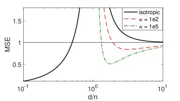
Figure 2: Surrogate MSE as a function of $d/n$, with $n$ fixed to $100$ and varying $d$, for signal-to-noise ratio $\mathrm{SNR}=1$.

The most directly comparable to our setting is the recent work of Hastie et al. (2019). They study how varying the feature dimension affects the (asymptotic) generalization error for linear regression, however their analysis is limited to certain special settings such as an isotropic data distribution. As an additional point of comparison, in Figure 2 we plot the MSE expressions of Theorem 1 when varying the feature dimension $d$ (the setup is the same as in Figure 1). Our plots follow the trends outlined by Hastie et al. (2019) for the isotropic case (see their Figure 2), but the spectral decay of the covariance (captured by our new MSE expressions) has a significant effect on the descent curve. This leads to generalization in the under-determined regime even when the signal-to-noise ratio ($\mathrm{SNR}=\|\mathbf{w}^{*}\|^{2}/\sigma^{2}$) is 1, unlike suggested by Hastie et al. (2019).

RandNLA and DPPs. Randomized Numerical Linear Algebra (Drineas and Mahoney, 2016, 2017) has traditionally focused on obtaining purely algorithmic improvements for tasks such as least squares regression, but there has been growing interest in understanding the statistical properties of these randomized methods (Ma et al., 2015; Raskutti and Mahoney, 2016). Determinantal point processes (Kulesza and Taskar, 2012) have been recently shown to combine strong worst-case regression guarantees with elegant statistical properties (Dereziński and Warmuth, 2017). However, these results are limited to the over-determined setting (Dereziński et al., 2018, 2019, 2019) and ridge regression (Dereziński and Warmuth, 2018; Dereziński et al., 2019). Our results are also related to recent work on using DPPs to analyze the expectation of the inverse (Dereziński and Mahoney, 2019) and generalized inverse (Mutný et al., 2019) of a subsampled matrix.

Implicit regularization. The term implicit regularization typically refers to the notion that approximate computation can implicitly lead to statistical regularization. See Mahoney and Orecchia (2011); Perry and Mahoney (2011); Gleich and Mahoney (2014) and references therein for early work on the topic; and see Mahoney (2012) for an overview. More recently, often motivated by neural networks, there has been work on implicit regularization that typically considered SGD-based optimization algorithms. See, e.g., theoretical results (Neyshabur et al., 2014; Neyshabur, 2017; Soudry et al., 2018; Gunasekar et al., 2017; Arora et al., 2019; Kubo et al., 2019) as well as extensive empirical studies (Martin and Mahoney, 2018, 2019). The implicit regularization observed by us is different in that it is not caused by an inexact approximation algorithm (such as SGD) but rather by the selection of one out of many exact solutions (e.g., the minimum norm solution). In this context, most relevant are the asymptotic results of Kobak et al. (2018) and LeJeune et al. (2019).

3 Surrogate random designs

In this section, we provide the definition of our surrogate random design $S_{\mu}^{n}$, where $\mu$ is a $d$-variate probability measure and $n$ is the sample size. This distribution is used in place of the standard random design $\mu^{n}$ consisting of $n$ row vectors drawn independently from $\mu$.

Preliminaries. For an $n\times n$ matrix $\mathbf{A}$, we use $\mathrm{pdet}(\mathbf{A})$ to denote the pseudo-determinant of $\mathbf{A}$, which is the product of non-zero eigenvalues. For index subsets $\mathcal{I}$ and $\mathcal{J}$, we use $\mathbf{A}_{\mathcal{I},\mathcal{J}}$ to denote the submatrix of $\mathbf{A}$ with rows indexed by $\mathcal{I}$ and columns indexed by $\mathcal{J}$. We may write $\mathbf{A}_{\mathcal{I},*}$ to indicate that we take a subset of rows. We let $\mathbf{X}\sim\mu^{k}$ denote a $k\times d$ random matrix with rows drawn i.i.d. according to $\mu$, and the $i$th row is denoted as $\mathbf{x}_{i}^{\scriptscriptstyle{\top}}$. We also let $\mathbf{\Sigma}_{\mu}=\mathbb{E}_{\mu}[\mathbf{x}\mathbf{x}^{\scriptscriptstyle{\top}}]$, where $\mathbb{E}_{\mu}$ refers to the expectation with respect to $\mathbf{x}^{\scriptscriptstyle{\top}}\!\sim\mu$, assuming throughout that $\mathbf{\Sigma}_{\mu}$ is well-defined and positive definite. We use ${\operatorname{Poisson}}(\gamma)_{\leq a}$ as the Poisson distribution restricted to $[0,a]$, whereas ${\operatorname{Poisson}}(\gamma)_{\geq a}$ is restricted to $[a,\infty)$. We also let $\#(\mathbf{X})$ denote the number of rows of $\mathbf{X}$.

Definition 2.

Let $\mu$ satisfy Assumption 2 and let $K$ be a random variable over $\mathbb{Z}_{\geq 0}$. A determinantal design ${\bar{\mathbf{X}}}\sim{\mathrm{Det}}(\mu,K)$ is a distribution with the same domain as $\mathbf{X}\sim\mu^{K}$ such that for any event $E$ measurable w.r.t. $\mathbf{X}$, we have

$$\mathrm{Pr}\big{\{}{\bar{\mathbf{X}}}\in E\big{\}}\ =\frac{\mathbb{E}[\mathrm{pdet}(\mathbf{X}\mathbf{X}^{\scriptscriptstyle{\top}})\mathbf{1}_{[\mathbf{X}\in E]}]}{\mathbb{E}[\mathrm{pdet}(\mathbf{X}\mathbf{X}^{\scriptscriptstyle{\top}})]}.$$

The above definition can be interpreted as rescaling the density function of $\mu^{K}$ by the pseudo-determinant, and then renormalizing it. We now construct our surrogate design $S_{\mu}^{n}$ by appropriately selecting the random variable $K$. The obvious choice of $K=n$ does not result in simple closed form expressions for the MSE in the under-determined regime (i.e., $n<d$), which is the regime of primary interest to us. Instead, we derive our random variables $K$ from the Poisson distribution.

Definition 3.

For $\mu$ satisfying Assumption 2, define surrogate design $S_{\mu}^{n}$ as ${\mathrm{Det}}(\mu,K)$ where:

1. if $n<d$, then $K\sim{\operatorname{Poisson}}(\gamma_{n})_{\leq d}$ with $\gamma_{n}$ as the solution of $n=\mathrm{tr}(\mathbf{\Sigma}_{\mu}(\mathbf{\Sigma}_{\mu}+\frac{1}{\gamma_{n}}\mathbf{I})^{-1})$,

2. if $n=d$, then we simply let $K=d$,

3. if $n>d$, then $K\sim{\operatorname{Poisson}}(\gamma_{n})_{\geq d}$ with $\gamma_{n}=n-d$.

Note that the under-determined case, i.e., $n<d$, is restricted to $K\leq d$ so that, under Assumption 2, $\mathrm{pdet}(\mathbf{X}\mathbf{X}^{\scriptscriptstyle{\top}})=\det(\mathbf{X}\mathbf{X}^{\scriptscriptstyle{\top}})$ with probability 1. On the other hand in the over-determined case, i.e., $n>d$, we have $K\geq d$ so that $\mathrm{pdet}(\mathbf{X}\mathbf{X}^{\scriptscriptstyle{\top}})=\det(\mathbf{X}^{\scriptscriptstyle{\top}}\mathbf{X})$. In the special case of $n=d=K$ both of these equations are satisfied: $\mathrm{pdet}(\mathbf{X}\mathbf{X}^{\scriptscriptstyle{\top}})=\det(\mathbf{X}^{\scriptscriptstyle{\top}}\mathbf{X})=\det(\mathbf{X}\mathbf{X}^{\scriptscriptstyle{\top}})=\det(\mathbf{X})^{2}$.

The first non-trivial property of the surrogate design $S_{\mu}^{n}$ is that the expected sample size is in fact always equal to $n$, which we prove in Appendix A.

Lemma 1.

Let ${\bar{\mathbf{X}}}\sim S_{\mu}^{n}$ for any $n>0$. Then, we have $\mathbb{E}[\#({\bar{\mathbf{X}}})]=n$.

Our general template for computing expectations under a surrogate design ${\bar{\mathbf{X}}}\sim\mathbf{S}_{\mu}^{n}$ is to use the following expressions based on the i.i.d. random design $\mathbf{X}\sim\mu^{K}$:

$$\mathbb{E}[F({\bar{\mathbf{X}}})] =\begin{cases}\frac{\mathbb{E}[\det(\mathbf{X}\mathbf{X}^{\scriptscriptstyle{\top}})F(\mathbf{X})]}{\mathbb{E}[\det(\mathbf{X}\mathbf{X}^{\scriptscriptstyle{\top}})]}\quad K\sim{\operatorname{Poisson}}(\gamma_{n})&\text{for }n<d,\\[5.69054pt] \frac{\mathbb{E}[\det(\mathbf{X})^{2}F(\mathbf{X})]}{\mathbb{E}[\det(\mathbf{X})^{2}]}\hskip 8.53581pt\quad K=d&\text{for }n=d,\\[5.69054pt] \frac{\mathbb{E}[\det(\mathbf{X}^{\scriptscriptstyle{\top}}\mathbf{X})F(\mathbf{X})]}{\mathbb{E}[\det(\mathbf{X}^{\scriptscriptstyle{\top}}\mathbf{X})]}\quad K\sim{\operatorname{Poisson}}(\gamma_{n})&\text{for }n>d.\end{cases}$$ (1)

These formulas follow from Definitions 2 and 3 because the determinants $\det(\mathbf{X}\mathbf{X}^{\scriptscriptstyle{\top}})$ and $\det(\mathbf{X}^{\scriptscriptstyle{\top}}\mathbf{X})$ are non-zero precisely in the regimes $n\leq d$ and $n\geq d$, respectively, which is why we can drop the restrictions on the range of the Poisson distribution. We compute the normalization constants by introducing the concept of determinant preserving random matrices, discussed in Section 4.

Proof sketch of Theorem 1

We focus here on the under-determined regime (i.e., $n<d$), highlighting the key new expectation formulas we develop to derive the MSE expressions for surrogate designs. A standard decomposition of the MSE yields:

$${\mathrm{MSE}\big{[}{\bar{\mathbf{X}}}^{\dagger}\bar{\mathbf{y}}\big{]}} =\mathbb{E}\big{[}\|{\bar{\mathbf{X}}}^{\dagger}({\bar{\mathbf{X}}}\mathbf{w}^{*}+\boldsymbol{\xi})-\mathbf{w}^{*}\|^{2}\big{]}=\sigma^{2}\mathbb{E}\big{[}\mathrm{tr}\big{(}({\bar{\mathbf{X}}}^{\scriptscriptstyle{\top}}{\bar{\mathbf{X}}})^{\dagger}\big{)}\big{]}+\mathbf{w}^{*{\scriptscriptstyle{\top}}}\mathbb{E}\big{[}\mathbf{I}-{\bar{\mathbf{X}}}^{\dagger}{\bar{\mathbf{X}}}\big{]}\mathbf{w}^{*}.$$ (2)

Thus, our task is to find closed form expressions for the two expectations above. The latter, which is the expected projection onto the complement of the row-span of ${\bar{\mathbf{X}}}$, is proven in Appendix D.

Lemma 2.

If ${\bar{\mathbf{X}}}\sim S_{\mu}^{n}$ and $n<d$, then we have: $\mathbb{E}\big{[}\mathbf{I}-{\bar{\mathbf{X}}}^{\dagger}{\bar{\mathbf{X}}}\big{]}=(\gamma_{n}\mathbf{\Sigma}_{\mu}+\mathbf{I})^{-1}$.

No such expectation formula is known for i.i.d. designs, except when $\mu$ is an isotropic Gaussian. In Appendix D, we also prove a generalization of Lemma 2 which is then used to establish our implicit regularization result (Theorem 2). We next give an expectation formula for the trace of the Moore-Penrose inverse of the covariance matrix for a surrogate design (proof in Appendix C).

Lemma 3.

If ${\bar{\mathbf{X}}}\sim S_{\mu}^{n}$ and $n<d$, then: $\mathbb{E}\big{[}\mathrm{tr}\big{(}({\bar{\mathbf{X}}}^{\scriptscriptstyle{\top}}{\bar{\mathbf{X}}})^{\dagger}\big{)}\big{]}=\gamma_{n}\big{(}1-\det\!\big{(}(\tfrac{1}{\gamma_{n}}\mathbf{I}+\mathbf{\Sigma}_{\mu})^{-1}\mathbf{\Sigma}_{\mu}\big{)}\big{)}$.

Note the implicit regularization term which appears in both formulas, given by $\lambda_{n}=\frac{1}{\gamma_{n}}$. Since $n=\mathrm{tr}(\mathbf{\Sigma}_{\mu}(\mathbf{\Sigma}_{\mu}+\lambda_{n}\mathbf{I})^{-1})=d-\lambda_{n}\mathrm{tr}((\mathbf{\Sigma}_{\mu}+\lambda_{n}\mathbf{I})^{-1})$, it follows that $\lambda_{n}=(d-n)/\mathrm{tr}((\mathbf{\Sigma}_{\mu}+\lambda_{n}\mathbf{I})^{-1})$. Combining this with Lemmas 2 and 3, we recover the surrogate MSE expression in Theorem 1.

4 Determinant preserving random matrices

In this section, we introduce the key tool for computing expectation formulas of matrix determinants. It is used in our analysis of the surrogate design, and it should be of independent interest.

The key question motivating the following definition is: When does taking expectation commute with computing a determinant for a square random matrix?

Definition 4.

A random $d\times d$ matrix $\mathbf{A}$ is called determinant preserving (d.p.), if

$$\mathbb{E}\big{[}\!\det(\mathbf{A}_{\mathcal{I},\mathcal{J}})\big{]}=\det\!\big{(}\mathbb{E}[\mathbf{A}_{\mathcal{I},\mathcal{J}}]\big{)}\quad\text{for all }\mathcal{I},\mathcal{J}\subseteq[d]\text{ s.t. }|\mathcal{I}|=|\mathcal{J}|.$$

We next give a few simple examples to provide some intuition. First, note that every $1\times 1$ random matrix is determinant preserving simply because taking a determinant is an identity transfomation in one dimension. Similarly, every fixed matrix is determinant preserving because in this case taking the expectation is an identity transformation. In all other cases, however, Definition 4 has to be verified more carefully. Further examples (positive and negative) follow.

Example 1.

If $\mathbf{A}$ has i.i.d. Gaussian entries $a_{ij}\sim\mathcal{N}(0,1)$, then $\mathbf{A}$ is d.p. because $\mathbb{E}[\det(\mathbf{A})]=0$.

In fact, it can be shown that all random matrices with independent entries are determinant preserving. However, this is not a necessary condition.

Example 2.

Let $\mathbf{A}=s\,\mathbf{Z}$, where $\mathbf{Z}$ is fixed with $\mathrm{rank}(\mathbf{Z})=r$, and $s$ is a scalar random variable. Then for $|\mathcal{I}|=|\mathcal{J}|=r$ we have

$$\mathbb{E}\big{[}\det(s\,\mathbf{Z}_{\mathcal{I},\mathcal{J}})\big{]} =\mathbb{E}[s^{r}]\det(\mathbf{Z}_{\mathcal{I},\mathcal{J}})=\det\Big{(}\big{(}\mathbb{E}[s^{r}]\big{)}^{\frac{1}{r}}\,\mathbf{Z}_{\mathcal{I},\mathcal{J}}\Big{)},$$

so if $r=1$ then $\mathbf{A}$ is determinant preserving, whereas if $r>1$ and $\mathrm{Var}[s]>0$ then it is not.

To construct more complex examples, we show that determinant preserving random matrices are closed under addition and multiplication. The proof of this result is an extension of an existing argument, given by Dereziński and Mahoney (2019) in the proof of Lemma 7, for computing the expected determinant of the sum of rank-1 random matrices (proof in Appendix B).

Lemma 4 (Closure properties).

If $\mathbf{A}$ and $\mathbf{B}$ are independent and determinant preserving, then:

1. $\mathbf{A}+\mathbf{B}$ is determinant preserving,

2. $\mathbf{A}\mathbf{B}$ is determinant preserving.

Next, we introduce another important class of d.p. matrices: a sum of i.i.d. rank-1 random matrices with the number of i.i.d. samples being a Poisson random variable. Our use of the Poisson distribution is crucial for the below result to hold. It is an extension of an expectation formula given by Dereziński (2019) for sampling from discrete distributions (proof in Appendix B).

Lemma 5.

If $K$ is a Poisson random variable and $\mathbf{A},\mathbf{B}$ are random $K\times d$ matrices whose rows are sampled as an i.i.d. sequence of joint pairs of random vectors, then $\mathbf{A}^{\scriptscriptstyle{\top}}\mathbf{B}$ is d.p., and so:

$$\mathbb{E}\big{[}\det(\mathbf{A}^{\scriptscriptstyle{\top}}\mathbf{B})\big{]} =\det\!\big{(}\mathbb{E}[\mathbf{A}^{\scriptscriptstyle{\top}}\mathbf{B}]\big{)}.$$

Finally, we show the expectation formula needed for obtaining the normalization constant of the under-determined surrogate design, given in (1). The below result is more general than the normalization constant requires, because it allows the matrices $\mathbf{A}$ and $\mathbf{B}$ to be different (the constant is obtained by setting $\mathbf{A}=\mathbf{B}=\mathbf{X}\sim\mu^{K}$). In fact, we use this more general statement to show Theorems 1 and 2. The proof uses Lemmas 4 and 5 (see Appendix B).

Lemma 6.

If $K$ is a Poisson random variable and $\mathbf{A}$, $\mathbf{B}$ are random $K\times d$ matrices whose rows are sampled as an i.i.d. sequence of joint pairs of random vectors, then

$$\mathbb{E}\big{[}\det(\mathbf{A}\mathbf{B}^{\scriptscriptstyle{\top}})\big{]} =\mathrm{e}^{-\mathbb{E}[K]}\det\!\big{(}\mathbf{I}+\mathbb{E}[\mathbf{B}^{\scriptscriptstyle{\top}}\mathbf{A}]\big{)}.$$

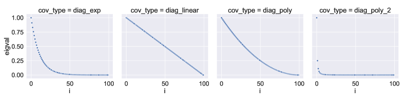
Figure 3: Scree-plots of $\mathbf{\Sigma}$ for the eigenvalue decays examined in our empirical valuations.

5 Empirical evaluation of asymptotic consistency

In this section, we empirically quantify the convergence rates for the asymptotic result of Theorem 3. We focus on the under-determined regime (i.e., $n<d$) and separate the evaluation into the bias and variance terms, following the MSE decomposition given in (2). Consider $\mathbf{X}=\mathbf{Z}\mathbf{\Sigma}^{1/2}$, where the entries of $\mathbf{Z}$ are i.i.d. standard Gaussian, and define:

1. Variance discrepancy: $\big{|}\frac{\mathbb{E}[\mathrm{tr}((\mathbf{X}^{\scriptscriptstyle{\top}}\mathbf{X})^{\dagger})]}{\mathcal{V}(\mathbf{\Sigma},n)}-1\big{|}$ where $\mathcal{V}(\mathbf{\Sigma},n)=\frac{1-\alpha_{n}}{\lambda_{n}}$.

2. Bias discrepancy: $\sup_{\mathbf{w}\in\mathbb{R}^{d}\backslash\{\mathbf{0}\}}\big{|}\frac{\mathbf{w}^{\scriptscriptstyle{\top}}\mathbb{E}[\mathbf{I}-\mathbf{X}^{\dagger}\mathbf{X}]\mathbf{w}}{\mathbf{w}^{\scriptscriptstyle{\top}}\mathcal{B}(\mathbf{\Sigma},n)\mathbf{w}}-1\big{|}$ where $\mathcal{B}(\mathbf{\Sigma},n)=\lambda_{n}(\mathbf{\Sigma}+\lambda_{n}\mathbf{I})^{-1}$.

Recall that $\lambda_{n}=\frac{d-n}{\mathrm{tr}((\mathbf{\Sigma}+\lambda_{n}\mathbf{I})^{-1})}$, so our surrogate MSE can be written as $\mathcal{M}=\sigma^{2}\mathcal{V}(\mathbf{\Sigma},n)+\mathbf{w}^{*{\scriptscriptstyle{\top}}}\mathcal{B}(\mathbf{\Sigma},n)\mathbf{w}^{*}$, and when both discrepancies are bounded by $\epsilon$, then $(1-2\epsilon)\mathcal{M}\leq{\mathrm{MSE}\big{[}\mathbf{X}^{\dagger}\mathbf{y}\big{]}}\leq(1+2\epsilon)\mathcal{M}$. In our experiments, we consider four standard eigenvalue decay profiles for $\mathbf{\Sigma}$, including polynomial and exponential decay (see Figure 3 and Section F.1).

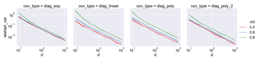
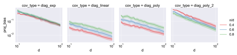
Figure 4: Empirical verification of the asymptotic consistency of surrogate MSE. We show the discrepancies for the variance (top) and bias (bottom), with bootstrapped $95\%$ confidence intervals, as $d$ increases and $n/d$ is fixed. We observe $O(1/d)$ decay (linear with slope $-1$ on a log-log plot).

Figure 4 (top) plots the variance discrepancy (with $\mathbb{E}[\mathrm{tr}((\mathbf{X}^{\scriptscriptstyle{\top}}\mathbf{X})^{\dagger})]$ estimated via Monte Carlo sampling and bootstrapped confidence intervals) as $d$ increases from $10$ to $1000$, across a range of aspect ratios $n/d$. In all cases, we observe that the discrepancy decays to zero at a rate of $O(1/d)$. Figure 4 (bottom) plots the bias discrepancy, with the same rate of decay observed throughout. Note that the range of $d$ is smaller than in Figure 4 (top) because the large number of Monte Carlo samples (up to two million) required for this experiment made the computations much more expensive (more details in Appendix F). Based on the above empirical results, we conclude with a conjecture.

Conjecture 1.

When $\mu$ is a centered multivariate Gaussian and its covariance has a constant condition number, then, for $n/d$ fixed, the surrogate MSE satisfies: $\big{|}\frac{\textnormal{MSE}[\mathbf{X}^{\dagger}\mathbf{y}]}{\mathcal{M}}-1\big{|}=O(1/d)$.

6 Conclusions

We derived exact non-asymptotic expressions for the MSE of the Moore-Penrose estimator in the linear regression task, reproducing the double descent phenomenon as the sample size crosses between the under- and over-determined regime. To achieve this, we modified the standard i.i.d. random design distribution using a determinantal point process to obtain a surrogate design which admits exact MSE expressions, while capturing the key properties of the i.i.d. design. We also provided a result that relates the expected value of the Moore-Penrose estimator of a training sample in the under-determined regime (i.e., the minimum norm solution) to the ridge-regularized least squares solution for the population distribution, thereby providing an interpretation for the implicit regularization resulting from over-parameterization.

Acknowledgements.

We would like to acknowledge ARO, DARPA, NSF, ONR, and GFSD for providing partial support of this work. We also thank Zhenyu Liao for pointing out fruitful connections between our results and the asymptotic analysis of random matrix resolvents.

Appendix A Proof of Lemma 1

We first record an important property of the design $S_{\mu}^{d}$ which can be used to construct an over-determined design for any $n>d$. A similar version of this result was also previously shown by Dereziński et al. (2019) for a different determinantal design.

Lemma 7.

Let ${\bar{\mathbf{X}}}\sim S_{\mu}^{d}$ and $\mathbf{X}\sim\mu^{K}$, where $K\sim{\operatorname{Poisson}}(\gamma)$. Then the matrix composed of a random permutation of the rows from ${\bar{\mathbf{X}}}$ and $\mathbf{X}$ is distributed according to $S_{\mu}^{d+\gamma}$.

Proof  Let $\widetilde{\mathbf{X}}$ denote the matrix constructed from the permuted rows of ${\bar{\mathbf{X}}}$ and $\mathbf{X}$. Letting $\mathbf{Z}\sim\mu^{K+d}$, we derive the probability $\mathrm{Pr}\big{\{}\widetilde{\mathbf{X}}\!\in\!E\big{\}}$ by summing over the possible index subsets $S\subseteq[K+d]$ that correspond to the rows coming from ${\bar{\mathbf{X}}}$:

$$\mathrm{Pr}\big{\{}\widetilde{\mathbf{X}}\in E\big{\}} =\mathbb{E}\bigg{[}\frac{1}{\binom{K+d}{d}}\sum_{S:\,|S|=d}\frac{\mathbb{E}[\det(\mathbf{Z}_{S,*})^{2}\mathbf{1}_{[\mathbf{Z}\in E]}\mid K]}{d!\det(\mathbf{\Sigma}_{\mu})}\bigg{]}$$

$$=\sum_{k=0}^{\infty}\frac{\gamma^{k}\mathrm{e}^{-\gamma}}{k!}\,\frac{\gamma^{d}k!}{(k+d)!}\,\frac{\mathbb{E}\big{[}\sum_{S:\,|S|=d}\det(\mathbf{Z}_{S,*})^{2}\mathbf{1}_{[\mathbf{Z}\in E]}\mid K=k\big{]}}{\det(\gamma\mathbf{\Sigma}_{\mu})}$$

$$\overset{(*)}{=}\sum_{k=0}^{\infty}\frac{\gamma^{k+d}\mathrm{e}^{-\gamma}}{(k+d)!}\,\frac{\mathbb{E}[\det(\mathbf{Z}^{\scriptscriptstyle{\top}}\mathbf{Z})\mathbf{1}_{[\mathbf{Z}\in E]}\mid K=k]}{\det(\gamma\mathbf{\Sigma}_{\mu})},$$

where $(*)$ uses the Cauchy-Binet formula to sum over all subsets $S$ of size $d$. Finally, since the sum shifts from $k$ to $k+d$, the last expression can be rewritten as $\mathbb{E}[\det(\mathbf{X}^{\scriptscriptstyle{\top}}\mathbf{X})\mathbf{1}_{[\mathbf{X}\in E]}]/\det(\gamma\mathbf{\Sigma}_{\mu})$, where recall that $\mathbf{X}\sim\mu^{K}$ and $K\sim{\operatorname{Poisson}}(\gamma)$, matching the definition of $S_{\mu}^{d+\gamma}$.  

We now proceed with the proof of Lemma 1, where we establish that the expected sample size of $S_{\mu}^{n}$ is indeed $n$.

Proof of Lemma 1  The result is obvious when $n=d$, whereas for $n>d$ it is an immediate consequence of Lemma 7. Finally, for $n<d$ the expected sample size follows as a corollary of Lemma 2, which states that

$$\text{(Lemma \ref{l:proj})}\qquad\mathbb{E}\big{[}\mathbf{I}-{\bar{\mathbf{X}}}^{\dagger}{\bar{\mathbf{X}}}\big{]}=(\gamma_{n}\mathbf{\Sigma}_{\mu}+\mathbf{I})^{-1},$$

where ${\bar{\mathbf{X}}}^{\dagger}{\bar{\mathbf{X}}}$ is the orthogonal projection onto the subspace spanned by the rows of ${\bar{\mathbf{X}}}$. Since the rank of this subspace is equal to the number of the rows, we have $\#({\bar{\mathbf{X}}})=\mathrm{tr}({\bar{\mathbf{X}}}^{\dagger}{\bar{\mathbf{X}}})$, so

$$\mathbb{E}\big{[}\#({\bar{\mathbf{X}}})\big{]}=d-\mathrm{tr}\big{(}(\gamma_{n}\mathbf{\Sigma}_{\mu}+\mathbf{I})^{-1}\big{)}=\mathrm{tr}\big{(}\gamma_{n}\mathbf{\Sigma}_{\mu}(\gamma_{n}\mathbf{\Sigma}_{\mu}+\mathbf{I})^{-1}\big{)}=n,$$

which completes the proof.  

Appendix B Proofs for Section 4

We use $\operatorname{\textnormal{adj}}(\mathbf{A})$ to denote the adjugate of $\mathbf{A}$, defined as follows: the $(i,j)$th entry of $\operatorname{\textnormal{adj}}(\mathbf{A})$ is $(-1)^{i+j}\det(\mathbf{A}_{[n]\backslash\{j\},[n]\backslash\{i\}})$. We will use two useful identities related to the adjugate: (1) $\operatorname{\textnormal{adj}}(\mathbf{A})=\det(\mathbf{A})\mathbf{A}^{-1}$ for invertible $\mathbf{A}$, and (2) $\det(\mathbf{A}+\mathbf{u}\mathbf{v}^{\scriptscriptstyle{\top}})=\det(\mathbf{A})+\mathbf{v}^{\scriptscriptstyle{\top}}\!\operatorname{\textnormal{adj}}(\mathbf{A})\mathbf{u}$ (see Fact 2.14.2 in Bernstein, 2011).

First, note that from the definition of an adjugate matrix it immediately follows that if $\mathbf{A}$ is determinant preserving then adjugate commutes with expectation for this matrix:

$$\mathbb{E}\big{[}\big{(}\!\operatorname{\textnormal{adj}}(\mathbf{A})\big{)}_{i,j}\big{]} =\mathbb{E}\big{[}(-1)^{i+j}\det(\mathbf{A}_{[d]\backslash\{j\},[d]\backslash\{i\}})\big{]}$$

$$=(-1)^{i+j}\det\!\big{(}\mathbb{E}[\mathbf{A}_{[d]\backslash\{j\},[d]\backslash\{i\}}]\big{)}$$ (3)

$$=\big{(}\!\operatorname{\textnormal{adj}}(\mathbb{E}[\mathbf{A}])\big{)}_{i,j}.$$ (4)

Proof of Lemma 4   First, we show that $\mathbf{A}+\mathbf{u}\mathbf{v}^{\scriptscriptstyle{\top}}$ is d.p. for any fixed $\mathbf{u},\mathbf{v}\in\mathbb{R}^{d}$. Below, we use the identity for a rank one update of a determinant: $\det(\mathbf{A}+\mathbf{u}\mathbf{v}^{\scriptscriptstyle{\top}})=\det(\mathbf{A})+\mathbf{v}^{\scriptscriptstyle{\top}}\!\operatorname{\textnormal{adj}}(\mathbf{A})\mathbf{u}$. It follows that for any $\mathcal{I}$ and $\mathcal{J}$ of the same size,

$$\mathbb{E}\big{[}\!\det(\mathbf{A}_{\mathcal{I},\mathcal{J}}\!+\mathbf{u}_{\mathcal{I}}\mathbf{v}_{\mathcal{J}}^{\scriptscriptstyle{\top}})\big{]} =\mathbb{E}\big{[}\!\det(\mathbf{A}_{\mathcal{I},\mathcal{J}})+\mathbf{v}_{\mathcal{J}}^{\scriptscriptstyle{\top}}\operatorname{\textnormal{adj}}(\mathbf{A}_{\mathcal{I},\mathcal{J}})\mathbf{u}_{\mathcal{I}}\big{]}$$

$$\overset{(*)}{=}\det\!\big{(}\mathbb{E}[\mathbf{A}_{\mathcal{I},\mathcal{J}}]\big{)}+\mathbf{v}_{\mathcal{J}}^{\scriptscriptstyle{\top}}\operatorname{\textnormal{adj}}\!\big{(}\mathbb{E}[\mathbf{A}_{\mathcal{I},\mathcal{J}}]\big{)}\mathbf{u}_{\mathcal{I}}$$

$$=\det\!\big{(}\mathbb{E}[\mathbf{A}_{\mathcal{I},\mathcal{J}}\!+\mathbf{u}_{\mathcal{I}}\mathbf{v}_{\mathcal{J}}^{\scriptscriptstyle{\top}}]\big{)},$$

where $(*)$ used (4), i.e., the fact that for d.p. matrices, adjugate commutes with expectation. Crucially, through the definition of an adjugate this step implicitly relies on the assumption that all the square submatrices of $\mathbf{A}_{\mathcal{I},\mathcal{J}}$ are also determinant preserving. Iterating this, we get that $\mathbf{A}+\mathbf{Z}$ is d.p. for any fixed $\mathbf{Z}$. We now show the same for $\mathbf{A}+\mathbf{B}$:

$$\mathbb{E}\big{[}\!\det(\mathbf{A}_{\mathcal{I},\mathcal{J}}\!+\mathbf{B}_{\mathcal{I},\mathcal{J}})\big{]} =\mathbb{E}\Big{[}\mathbb{E}\big{[}\!\det(\mathbf{A}_{\mathcal{I},\mathcal{J}}\!+\mathbf{B}_{\mathcal{I},\mathcal{J}})\mid\mathbf{B}\big{]}\Big{]}$$

$$\overset{(*)}{=}\mathbb{E}\Big{[}\!\det\!\big{(}\mathbb{E}[\mathbf{A}_{\mathcal{I},\mathcal{J}}]\!+\mathbf{B}_{\mathcal{I},\mathcal{J}}\big{)}\Big{]}$$

$$=\det\!\big{(}\mathbb{E}[\mathbf{A}_{\mathcal{I},\mathcal{J}}\!+\mathbf{B}_{\mathcal{I},\mathcal{J}}]\big{)},$$

where $(*)$ uses the fact that after conditioning on $\mathbf{B}$ we can treat it as a fixed matrix. Next, we show that $\mathbf{A}\mathbf{B}$ is determinant preserving via the Cauchy-Binet formula:

$$\mathbb{E}\big{[}\!\det\!\big{(}(\mathbf{A}\mathbf{B})_{\mathcal{I},\mathcal{J}}\big{)}\big{]} =\mathbb{E}\big{[}\!\det(\mathbf{A}_{\mathcal{I},*}\mathbf{B}_{*,\mathcal{J}})\big{]}$$

$$=\mathbb{E}\bigg{[}\sum_{S:\,|S|=|\mathcal{I}|}\!\!\det\!\big{(}\mathbf{A}_{\mathcal{I},S}\big{)}\det\!\big{(}\mathbf{B}_{S,\mathcal{J}}\big{)}\bigg{]}$$

$$=\!\!\sum_{S:\,|S|=|\mathcal{I}|}\!\!\det\!\big{(}\mathbb{E}[\mathbf{A}]_{\mathcal{I},S}\big{)}\det\!\big{(}\mathbb{E}[\mathbf{B}]_{S,\mathcal{J}}\big{)}$$

$$=\det\!\big{(}\mathbb{E}[\mathbf{A}]_{\mathcal{I},*}\,\mathbb{E}[\mathbf{B}]_{*,\mathcal{J}}\big{)}$$

$$=\det\!\big{(}\mathbb{E}[\mathbf{A}\mathbf{B}]_{\mathcal{I},\mathcal{J}}\big{)},$$

where recall that $\mathbf{A}_{\mathcal{I},*}$ denotes the submatrix of $\mathbf{A}$ consisting of its (entire) rows indexed by $\mathcal{I}$.  

To prove Lemma 5, we will use the following lemma, many variants of which appeared in the literature (e.g., van der Vaart, 1965). We use the one given by Dereziński et al. (2019).

Lemma 8 (Dereziński et al. (2019)).

If the rows of random $k\times d$ matrices $\mathbf{A},\mathbf{B}$ are sampled as an i.i.d. sequence of $k\geq d$ pairs of joint random vectors, then

$$k^{d}\,\mathbb{E}\big{[}\det(\mathbf{A}^{\scriptscriptstyle{\top}}\mathbf{B})\big{]} ={k^{\underline{d}}}\,\det\!\big{(}\mathbb{E}[\mathbf{A}^{\scriptscriptstyle{\top}}\mathbf{B}]\big{)}.$$ (5)

Here, we use the following standard shorthand: ${k^{\underline{d}}}=\frac{k!}{(k-d)!}=k\,(k-1)\dotsm(k-d+1)$. Note that the above result almost looks like we are claiming that the matrix $\mathbf{A}^{\scriptscriptstyle{\top}}\mathbf{B}$ is d.p., but in fact it is not because $k^{d}\neq{k^{\underline{d}}}$. The difference in those factors is precisely what we are going to correct with the Poisson random variable. We now present the proof of Lemma 5.

Proof of Lemma 5  Without loss of generality, it suffices to check Definition 4 with both $\mathcal{I}$ and $\mathcal{J}$ equal $[d]$. We first expand the expectation by conditioning on the value of $K$ and letting $\gamma=\mathbb{E}[K]$:

$$\mathbb{E}\big{[}\!\det(\mathbf{A}^{\scriptscriptstyle{\top}}\mathbf{B})\big{]} =\sum_{k=0}^{\infty}\mathbb{E}\big{[}\det(\mathbf{A}^{\scriptscriptstyle{\top}}\mathbf{B})\mid K\!=\!k\big{]}\ \mathrm{Pr}(K\!=\!k)$$

(Lemma 8) $$=\sum_{k=d}^{\infty}\frac{k!k^{-d}}{(k-d)!}\det\!\big{(}\mathbb{E}[\mathbf{A}^{\scriptscriptstyle{\top}}\mathbf{B}\mid K\!=\!k]\big{)}\frac{\gamma^{k}\mathrm{e}^{-\gamma}}{k!}$$

$$=\sum_{k=d}^{\infty}\Big{(}\frac{\gamma}{k}\Big{)}^{d}\det\!\big{(}\mathbb{E}[\mathbf{A}^{\scriptscriptstyle{\top}}\mathbf{B}\mid K\!=\!k]\big{)}\frac{\gamma^{k-d}\mathrm{e}^{-\gamma}}{(k-d)!}.$$

Note that $\frac{\gamma}{k}\,\mathbb{E}[\mathbf{A}^{\scriptscriptstyle{\top}}\mathbf{B}\mid K\!=\!k]=\mathbb{E}[\mathbf{A}^{\scriptscriptstyle{\top}}\mathbf{B}]$, which is independent of $k$. Thus we can rewrite the above expression as:

$$\det\!\big{(}\mathbb{E}[\mathbf{A}^{\scriptscriptstyle{\top}}\mathbf{B}]\big{)}\sum_{k=d}^{\infty}\frac{\gamma^{k-d}\mathrm{e}^{-\gamma}}{(k-d)!}=\det\!\big{(}\mathbb{E}[\mathbf{A}^{\scriptscriptstyle{\top}}\mathbf{B}]\big{)}\sum_{k=0}^{\infty}\frac{\gamma^{k}\mathrm{e}^{-\gamma}}{k!}=\det\!\big{(}\mathbb{E}[\mathbf{A}^{\scriptscriptstyle{\top}}\mathbf{B}]\big{)},$$

which concludes the proof.  

To prove Lemma 6, we use the following standard determinantal formula which is used to derive the normalization constant of a discrete determinantal point process.

Lemma 9 (Kulesza and Taskar (2012)).

For any $k\times d$ matrices $\mathbf{A},\mathbf{B}$ we have

$$\det(\mathbf{I}+\mathbf{A}\mathbf{B}^{\scriptscriptstyle{\top}})=\sum_{S\subseteq[k]}\det(\mathbf{A}_{S,*}\mathbf{B}_{S,*}^{\scriptscriptstyle{\top}}).$$

Proof of Lemma 6  By Lemma 5, the matrix $\mathbf{B}^{\scriptscriptstyle{\top}}\mathbf{A}$ is determinant preserving. Applying Lemma 4 we conclude that $\mathbf{I}+\mathbf{B}^{\scriptscriptstyle{\top}}\mathbf{A}$ is also d.p., so

$$\det\!\big{(}\mathbf{I}+\mathbb{E}[\mathbf{B}^{\scriptscriptstyle{\top}}\mathbf{A}]\big{)}=\mathbb{E}\big{[}\det(\mathbf{I}+\mathbf{B}^{\scriptscriptstyle{\top}}\mathbf{A})\big{]}=\mathbb{E}\big{[}\det(\mathbf{I}+\mathbf{A}\mathbf{B}^{\scriptscriptstyle{\top}})\big{]},$$

where the second equality is known as Sylvester’s Theorem. We rewrite the expectation of $\det(\mathbf{I}+\mathbf{A}\mathbf{B}^{\scriptscriptstyle{\top}})$ by applying Lemma 9. Letting $\gamma=\mathbb{E}[K]$, we obtain:

$$\mathbb{E}\big{[}\det(\mathbf{I}+\mathbf{A}\mathbf{B}^{\scriptscriptstyle{\top}})\big{]} =\mathbb{E}\bigg{[}\sum_{S\subseteq[K]}\mathbb{E}\big{[}\det(\mathbf{A}_{S,*}\mathbf{B}_{S,*}^{\scriptscriptstyle{\top}})\mid K\big{]}\bigg{]}$$

$$\overset{(*)}{=}\sum_{k=0}^{\infty}\frac{\gamma^{k}\mathrm{e}^{-\gamma}}{k!}\sum_{i=0}^{k}\binom{k}{i}\mathbb{E}\big{[}\det(\mathbf{A}\mathbf{B}^{\scriptscriptstyle{\top}})\mid K=i\big{]}$$

$$=\sum_{i=0}^{\infty}\mathbb{E}\big{[}\det(\mathbf{A}\mathbf{B}^{\scriptscriptstyle{\top}})\mid K=i\big{]}\sum_{k\geq i}^{\infty}\binom{k}{i}\frac{\gamma^{k}\mathrm{e}^{-\gamma}}{k!}$$

$$=\sum_{i=0}^{\infty}\frac{\gamma^{i}\mathrm{e}^{-\gamma}}{i!}\mathbb{E}\big{[}\det(\mathbf{A}\mathbf{B}^{\scriptscriptstyle{\top}})\mid K=i\big{]}\sum_{k\geq i}^{\infty}\frac{\gamma^{k-i}}{(k-i)!}=\mathbb{E}\big{[}\det(\mathbf{A}\mathbf{B}^{\scriptscriptstyle{\top}})\big{]}\cdot\mathrm{e}^{\gamma},$$

where $(*)$ follows from the exchangeability of the rows of $\mathbf{A}$ and $\mathbf{B}$, which implies that the distribution of $\mathbf{A}_{S,*}\mathbf{B}_{S,*}^{\scriptscriptstyle{\top}}$ is the same for all subsets $S$ of a fixed size $k$.  

Appendix C Proof of Theorem 1

In this section we use $Z_{\mu}^{n}$ to denote the normalization constant that appears in (1) when computing an expectation for surrogate design $S_{\mu}^{n}$. We first prove Lemma 3.

Lemma 10 (restated Lemma 3).

If ${\bar{\mathbf{X}}}\sim S_{\mu}^{n}$ for $n<d$, then we have

$$\mathbb{E}\big{[}\mathrm{tr}\big{(}({\bar{\mathbf{X}}}^{\scriptscriptstyle{\top}}{\bar{\mathbf{X}}})^{\dagger}\big{)}\big{]} ={\gamma_{n}}\big{(}1-\det\!\big{(}(\tfrac{1}{\gamma_{n}}\mathbf{I}+\mathbf{\Sigma}_{\mu})^{-1}\mathbf{\Sigma}_{\mu}\big{)}\big{)}.$$

Proof  Let $\mathbf{X}\sim\mu^{K}$ for $K\sim{\operatorname{Poisson}}({\gamma_{n}})$. Note that if $\det(\mathbf{X}\mathbf{X}^{\scriptscriptstyle{\top}})>0$ then using the fact that $\det(\mathbf{A})\mathbf{A}^{-1}=\operatorname{\textnormal{adj}}(\mathbf{A})$ for any invertible matrix $\mathbf{A}$, we can write:

$$\det(\mathbf{X}\mathbf{X}^{\scriptscriptstyle{\top}})\mathrm{tr}\big{(}(\mathbf{X}^{\scriptscriptstyle{\top}}\mathbf{X})^{\dagger}\big{)} =\det(\mathbf{X}\mathbf{X}^{\scriptscriptstyle{\top}})\mathrm{tr}\big{(}(\mathbf{X}\mathbf{X}^{\scriptscriptstyle{\top}})^{-1}\big{)}$$

$$=\mathrm{tr}(\operatorname{\textnormal{adj}}(\mathbf{X}\mathbf{X}^{\scriptscriptstyle{\top}}))$$

$$=\sum_{i=1}^{K}\det(\mathbf{X}_{-i}\mathbf{X}_{-i}^{\scriptscriptstyle{\top}}),$$

where $\mathbf{X}_{-i}$ is a shorthand for $\mathbf{X}_{[K]\backslash\{i\},*}$. Assumption 2 ensures that $\mathrm{Pr}\big{\{}\det(\mathbf{X}\mathbf{X}^{\scriptscriptstyle{\top}})>0\big{\}}=1$, which allows us to write:

$$Z_{\mu}^{n}\cdot\mathbb{E}\big{[}\mathrm{tr}\big{(}({\bar{\mathbf{X}}}^{\scriptscriptstyle{\top}}{\bar{\mathbf{X}}})^{\dagger}\big{)}\big{]} =\mathbb{E}\bigg{[}\sum_{i=1}^{K}\det(\mathbf{X}_{-i}\mathbf{X}_{-i}^{\scriptscriptstyle{\top}})\ \big{|}\ \det(\mathbf{X}\mathbf{X}^{\scriptscriptstyle{\top}})>0\bigg{]}\cdot\overbrace{\mathrm{Pr}\big{\{}\det(\mathbf{X}\mathbf{X}^{\scriptscriptstyle{\top}})>0\big{\}}}^{1}$$

$$=\sum_{k=0}^{d}\frac{\gamma_{n}^{k}\mathrm{e}^{-\gamma_{n}}}{k!}\mathbb{E}\Big{[}\sum_{i=1}^{k}\det(\mathbf{X}_{-i}\mathbf{X}_{-i}^{\scriptscriptstyle{\top}})\ \big{|}\ K=k\Big{]}$$

$$=\sum_{k=0}^{d}\frac{\gamma_{n}^{k}\mathrm{e}^{-\gamma_{n}}}{k!}\,k\ \mathbb{E}\big{[}\det(\mathbf{X}\mathbf{X}^{\scriptscriptstyle{\top}})\mid K=k-1\big{]}$$

$$=\gamma_{n}\sum_{k=0}^{d-1}\frac{\gamma_{n}^{k}\mathrm{e}^{-\gamma_{n}}}{k!}\mathbb{E}\big{[}\det(\mathbf{X}\mathbf{X}^{\scriptscriptstyle{\top}})\mid K=k\big{]}$$

$$=\gamma_{n}\Big{(}\mathbb{E}\big{[}\det(\mathbf{X}\mathbf{X}^{\scriptscriptstyle{\top}})\big{]}\ -\ \frac{\gamma_{n}^{d}\mathrm{e}^{-\gamma_{n}}}{d!}\mathbb{E}\big{[}\det(\mathbf{X})^{2}\mid K=d\big{]}\Big{)}$$

$$\overset{(*)}{=}\gamma_{n}\big{(}\mathrm{e}^{-\gamma_{n}}\det(\mathbf{I}+\gamma_{n}\mathbf{\Sigma}_{\mu})-\mathrm{e}^{-\gamma_{n}}\det(\gamma_{n}\mathbf{\Sigma}_{\mu})\big{)},$$

where $(*)$ uses Lemma 6 for the first term and Lemma 8 for the second term. We obtain the desired result by dividing both sides by $Z_{\mu}^{n}=\mathrm{e}^{-\gamma_{n}}\det(\mathbf{I}+\gamma_{n}\mathbf{\Sigma}_{\mu})$.  

In the over-determined regime, a more general matrix expectation formula can be shown (omitting the trace). The following result is related to an expectation formula derived by Dereziński et al. (2019), however they use a slightly different determinantal design so the results are incomparable.

Lemma 11.

If ${\bar{\mathbf{X}}}\sim S_{\mu}^{n}$ and $n>d$, then we have

$$\mathbb{E}\big{[}({\bar{\mathbf{X}}}^{\scriptscriptstyle{\top}}{\bar{\mathbf{X}}})^{\dagger}\big{]}=\mathbf{\Sigma}_{\mu}^{-1}\cdot\frac{1-\mathrm{e}^{-\gamma_{n}}}{\gamma_{n}}.$$

Proof  Let $\mathbf{X}\sim\mu^{K}$ for $K\sim{\operatorname{Poisson}}(\gamma_{n})$. Assumption 2 implies that for $K\neq d-1$ we have

$$\det(\mathbf{X}^{\scriptscriptstyle{\top}}\mathbf{X})(\mathbf{X}^{\scriptscriptstyle{\top}}\mathbf{X})^{\dagger}=\operatorname{\textnormal{adj}}(\mathbf{X}^{\scriptscriptstyle{\top}}\mathbf{X}),$$ (6)

however when $k=d-1$ then (6) does not hold because $\det(\mathbf{X}^{\scriptscriptstyle{\top}}\mathbf{X})=0$ while $\operatorname{\textnormal{adj}}(\mathbf{X}^{\scriptscriptstyle{\top}}\mathbf{X})$ may be non-zero. It follows that:

$$Z_{\mu}^{n}\cdot\mathbb{E}\big{[}({\bar{\mathbf{X}}}^{\scriptscriptstyle{\top}}{\bar{\mathbf{X}}})^{\dagger}\big{]} =\mathbb{E}\big{[}\det(\mathbf{X}^{\scriptscriptstyle{\top}}\mathbf{X})(\mathbf{X}^{\scriptscriptstyle{\top}}\mathbf{X})^{\dagger}\big{]}$$

$$=\mathbb{E}\big{[}\operatorname{\textnormal{adj}}(\mathbf{X}^{\scriptscriptstyle{\top}}\mathbf{X})\big{]}-\frac{\gamma_{n}^{d-1}\mathrm{e}^{-\gamma_{n}}}{(d-1)!}\mathbb{E}\big{[}\operatorname{\textnormal{adj}}(\mathbf{X}^{\scriptscriptstyle{\top}}\mathbf{X})\mid K=d-1\big{]}$$

$$\overset{(*)}{=}\operatorname{\textnormal{adj}}\!\big{(}\mathbb{E}[\mathbf{X}^{\scriptscriptstyle{\top}}\mathbf{X}]\big{)}-\frac{\gamma_{n}^{d-1}\mathrm{e}^{-\gamma_{n}}}{(d-1)^{d-1}}\operatorname{\textnormal{adj}}\!\big{(}\mathbb{E}[\mathbf{X}^{\scriptscriptstyle{\top}}\mathbf{X}\mid K=d-1]\big{)}$$

$$=\operatorname{\textnormal{adj}}(\gamma_{n}\mathbf{\Sigma}_{\mu})-\mathrm{e}^{-\gamma_{n}}\operatorname{\textnormal{adj}}(\gamma_{n}\mathbf{\Sigma}_{\mu})$$

$$=\det(\gamma_{n}\mathbf{\Sigma}_{\mu})\,(\gamma_{n}\mathbf{\Sigma}_{\mu})^{-1}(1-\mathrm{e}^{-\gamma_{n}})$$

$$=\det(\gamma_{n}\mathbf{\Sigma}_{\mu})\,\mathbf{\Sigma}_{\mu}^{-1}\cdot\frac{1-\mathrm{e}^{-\gamma_{n}}}{\gamma_{n}},$$

where the first term in $(*)$ follows from Lemma 6 and (4), whereas the second term comes from Lemma 2.3 of Dereziński et al. (2019). Dividing both sides by $Z_{\mu}^{n}=\det(\gamma_{n}\mathbf{\Sigma}_{\mu})$ completes the proof.  

Applying the closed form expressions from Lemmas 2, 3 and 11, we derive the formula for the MSE and prove Theorem 1 (we defer the proof of Lemma 2 to Appendix D).

Proof of Theorem 1  First, assume that $n<d$, in which case we have $\gamma_{n}=\frac{1}{\lambda_{n}}$ and moreover

$$n =\mathrm{tr}\big{(}\mathbf{\Sigma}_{\mu}(\mathbf{\Sigma}_{\mu}+\lambda_{n}\mathbf{I})^{-1}\big{)}$$

$$=\mathrm{tr}\big{(}(\mathbf{\Sigma}_{\mu}+\lambda_{n}\mathbf{I}-\lambda_{n}\mathbf{I})(\mathbf{\Sigma}_{\mu}+\lambda_{n}\mathbf{I})^{-1}\big{)}$$

$$=d-\lambda_{n}\mathrm{tr}\big{(}(\mathbf{\Sigma}_{\mu}+\lambda_{n}\mathbf{I})^{-1}\big{)},$$

so we can write $\lambda_{n}$ as $(d-n)/\mathrm{tr}((\mathbf{\Sigma}_{\mu}+\lambda_{n}\mathbf{I})^{-1})$. From this and Lemmas 2 and 10, we obtain the desired expression, where recall that $\alpha_{n}=\det\!\big{(}\mathbf{\Sigma}_{\mu}(\mathbf{\Sigma}_{\mu}+\frac{1}{\gamma_{n}})^{-1}\big{)}$:

$${\mathrm{MSE}\big{[}{\bar{\mathbf{X}}}^{\dagger}\bar{\mathbf{y}}\big{]}} =\sigma^{2}\,\gamma_{n}(1-\alpha_{n})+\tfrac{1}{\gamma_{n}}\,\mathbf{w}^{*{\scriptscriptstyle{\top}}}(\mathbf{\Sigma}_{\mu}+\tfrac{1}{\gamma_{n}}\mathbf{I})^{-1}\mathbf{w}^{*}$$

$$\overset{(a)}{=}\sigma^{2}\,\frac{1-\alpha_{n}}{\lambda_{n}}+\lambda_{n}\,\mathbf{w}^{*{\scriptscriptstyle{\top}}}(\mathbf{\Sigma}_{\mu}+\lambda_{n}\mathbf{I})^{-1}\mathbf{w}^{*}$$

$$\overset{(b)}{=}\sigma^{2}\mathrm{tr}\big{(}(\mathbf{\Sigma}_{\mu}+\lambda_{n}\mathbf{I})^{-1}\big{)}\frac{1-\alpha_{n}}{d-n}+(d-n)\frac{\mathbf{w}^{*{\scriptscriptstyle{\top}}}(\mathbf{\Sigma}_{\mu}+\lambda_{n}\mathbf{I})^{-1}\mathbf{w}^{*}}{\mathrm{tr}\big{(}(\mathbf{\Sigma}_{\mu}+\lambda_{n}\mathbf{I})^{-1}\big{)}}.$$

While the expression given after $(a)$ is simpler than the one after $(b)$, the latter better illustrates how the MSE depends on the sample size $n$ and the dimension $d$. Now, assume that $n>d$. In this case, we have $\gamma_{n}=n-d$ and apply Lemma 11:

$${\mathrm{MSE}\big{[}{\bar{\mathbf{X}}}^{\dagger}\bar{\mathbf{y}}\big{]}} =\sigma^{2}\,\mathrm{tr}(\mathbf{\Sigma}_{\mu}^{-1})\,\frac{1-\mathrm{e}^{-\gamma_{n}}}{\gamma_{n}}=\sigma^{2}\,\mathrm{tr}(\mathbf{\Sigma}_{\mu}^{-1})\,\frac{1-\beta_{n}}{n-d}.$$

The case of $n=d$ was shown in Theorem 2.12 of Dereziński et al. (2019). This concludes the proof.  

Appendix D Proof of Theorem 2

As in the previous section, we use $Z_{\mu}^{n}$ to denote the normalization constant that appears in (1) when computing an expectation for surrogate design $S_{\mu}^{n}$. Recall that our goal is to compute the expected value of ${\bar{\mathbf{X}}}^{\dagger}\bar{\mathbf{y}}$ under the surrogate design $S_{\mu}^{n}$. Similarly as for Theorem 1, the case of $n=d$ was shown in Theorem 2.10 of Dereziński et al. (2019). We break the rest down into the under-determined case $(n<d)$ and the over-determined case ($n>d$), starting with the former. Recall that we do not require any modeling assumptions on the responses.

Lemma 12.

If ${\bar{\mathbf{X}}}\sim S_{\mu}^{n}$ and $n<d$, then for any $y(\cdot)$ such that $\mathbb{E}_{\mu,y}[y(\mathbf{x})\,\mathbf{x}]$ is well-defined, denoting ${\bar{y}}_{i}$ as $y(\bar{\mathbf{x}}_{i})$, we have

$$\mathbb{E}\big{[}{\bar{\mathbf{X}}}^{\dagger}\bar{\mathbf{y}}\big{]} =\big{(}\mathbf{\Sigma}_{\mu}+\tfrac{1}{\gamma_{n}}\mathbf{I}\big{)}^{-1}\mathbb{E}_{\mu,y}[y(\mathbf{x})\,\mathbf{x}].$$

Proof  Let $\mathbf{X}\sim\mu^{K}$ for $K\sim{\operatorname{Poisson}}(\gamma_{n})$ and denote $y(\mathbf{x}_{i})$ as $y_{i}$. Note that when $\det(\mathbf{X}\mathbf{X}^{\scriptscriptstyle{\top}})>0$, then the $j$th entry of $\mathbf{X}^{\dagger}\mathbf{y}$ equals $\mathbf{f}_{j}^{\scriptscriptstyle{\top}}(\mathbf{X}\mathbf{X}^{\scriptscriptstyle{\top}})^{-1}\mathbf{y}$, where $\mathbf{f}_{j}$ is the $j$th column of $\mathbf{X}$, so:

$$\det(\mathbf{X}\mathbf{X}^{\scriptscriptstyle{\top}})\,(\mathbf{X}^{\dagger}\mathbf{y})_{j} =\det(\mathbf{X}\mathbf{X}^{\scriptscriptstyle{\top}})\,\mathbf{f}_{j}^{\scriptscriptstyle{\top}}(\mathbf{X}\mathbf{X}^{\scriptscriptstyle{\top}})^{-1}\mathbf{y}$$

$$=\det(\mathbf{X}\mathbf{X}^{\scriptscriptstyle{\top}}+\mathbf{y}\mathbf{f}_{j}^{\scriptscriptstyle{\top}})-\det(\mathbf{X}\mathbf{X}^{\scriptscriptstyle{\top}}).$$

If $\det(\mathbf{X}\mathbf{X}^{\scriptscriptstyle{\top}})=0$, then also $\det(\mathbf{X}\mathbf{X}^{\scriptscriptstyle{\top}}+\mathbf{y}\mathbf{f}_{j}^{\scriptscriptstyle{\top}})=0$, so we can write:

$$Z_{\mu}^{n}\cdot\mathbb{E}\big{[}({\bar{\mathbf{X}}}^{\dagger}\bar{\mathbf{y}})_{j}\big{]} =\mathbb{E}\big{[}\det(\mathbf{X}\mathbf{X}^{\scriptscriptstyle{\top}})(\mathbf{X}^{\dagger}\mathbf{y})_{j}\big{]}$$

$$=\mathbb{E}\big{[}\det(\mathbf{X}\mathbf{X}^{\scriptscriptstyle{\top}}+\mathbf{y}\mathbf{f}_{j}^{\scriptscriptstyle{\top}})-\det(\mathbf{X}\mathbf{X}^{\scriptscriptstyle{\top}})\big{]}$$

$$=\mathbb{E}\big{[}\det\!\big{(}[\mathbf{X},\mathbf{y}][\mathbf{X},\mathbf{f}_{j}]^{\scriptscriptstyle{\top}}\big{)}\big{]}-\mathbb{E}\big{[}\det(\mathbf{X}\mathbf{X}^{\scriptscriptstyle{\top}})\big{]}$$

$$\overset{(a)}{=}\mathrm{e}^{-\gamma_{n}}\det\!\bigg{(}\mathbf{I}+\gamma_{n}\,\mathbb{E}_{\mu,y}\bigg{[}\begin{pmatrix}\mathbf{x}\mathbf{x}^{\scriptscriptstyle{\top}}&\!\!\mathbf{x}\,y(\mathbf{x})\\ x_{j}\,\mathbf{x}^{\scriptscriptstyle{\top}}&\!\!x_{j}\,y(\mathbf{x})\end{pmatrix}\bigg{]}\bigg{)}-\mathrm{e}^{-\gamma_{n}}\det(\mathbf{I}+\gamma_{n}\mathbf{\Sigma}_{\mu})$$

$$\overset{(b)}{=}\mathrm{e}^{-\gamma_{n}}\det(\mathbf{I}+\gamma_{n}\mathbf{\Sigma}_{\mu})$$

$$\qquad\times\Big{(}\mathbb{E}_{\mu,y}\big{[}\gamma_{n}x_{j}\,y(\mathbf{x})\big{]}-\mathbb{E}_{\mu}\big{[}\gamma_{n}x_{j}\,\mathbf{x}^{\scriptscriptstyle{\top}}\big{]}(\mathbf{I}+\gamma_{n}\mathbf{\Sigma}_{\mu})^{-1}\mathbb{E}_{\mu,y}\big{[}\gamma_{n}\mathbf{x}\,y(\mathbf{x})\big{]}\Big{)},$$

where $(a)$ uses Lemma 6 twice, with the first application involving two different matrices $\mathbf{A}=[\mathbf{X},\mathbf{y}]$ and $\mathbf{B}=[\mathbf{X},\mathbf{f}_{j}]$, whereas $(b)$ is a standard determinantal identity (see Fact 2.14.2 in Bernstein, 2011). Dividing both sides by $Z_{\mu}^{n}$ and letting $\mathbf{v}_{\mu,y}=\mathbb{E}_{\mu,y}[y(\mathbf{x})\,\mathbf{x}]$, we obtain that:

$$\mathbb{E}\big{[}{\bar{\mathbf{X}}}^{\dagger}\bar{\mathbf{y}}\big{]} =\gamma_{n}\mathbf{v}_{\mu,y}-\gamma_{n}^{2}\mathbf{\Sigma}_{\mu}(\mathbf{I}+\gamma_{n}\mathbf{\Sigma}_{\mu})^{-1}\mathbf{v}_{\mu,y}$$

$$=\gamma_{n}\big{(}\mathbf{I}-\gamma_{n}\mathbf{\Sigma}_{\mu}(\mathbf{I}+\gamma_{n}\mathbf{\Sigma}_{\mu})^{-1}\big{)}\mathbf{v}_{\mu,y}=\gamma_{n}(\mathbf{I}+\gamma_{n}\mathbf{\Sigma}_{\mu})^{-1}\mathbf{v}_{\mu,y},$$

which completes the proof.  

We return to Lemma 2, regarding the expected orthogonal projection onto the complement of the row-span of ${\bar{\mathbf{X}}}$, i.e., $\mathbb{E}[\mathbf{I}-{\bar{\mathbf{X}}}^{\dagger}{\bar{\mathbf{X}}}]$, which follows as a corollary of Lemma 12.

Proof of Lemma 2  We let $y(\mathbf{x})=x_{j}$ where $j\in[d]$ and apply Lemma 12 for each $j$, obtaining:

$$\mathbf{I}-\mathbb{E}\big{[}{\bar{\mathbf{X}}}^{\dagger}{\bar{\mathbf{X}}}]=\mathbf{I}-(\mathbf{\Sigma}_{\mu}+\tfrac{1}{\gamma_{n}}\mathbf{I})^{-1}\mathbf{\Sigma}_{\mu},$$

from which the result follows by simple algebraic manipulation.  

We move on to the over-determined case, where the ridge regularization of adding the identity to $\mathbf{\Sigma}_{\mu}$ vanishes. Recall that we assume throughout the paper that $\mathbf{\Sigma}_{\mu}$ is invertible.

Lemma 13.

If ${\bar{\mathbf{X}}}\sim S_{\mu}^{n}$ and $n>d$, then for any real-valued random function $y(\cdot)$ such that $\mathbb{E}_{\mu,y}[y(\mathbf{x})\,\mathbf{x}]$ is well-defined, denoting ${\bar{y}}_{i}$ as $y(\bar{\mathbf{x}}_{i})$, we have

$$\mathbb{E}\big{[}{\bar{\mathbf{X}}}^{\dagger}\bar{\mathbf{y}}\big{]} =\mathbf{\Sigma}_{\mu}^{-1}\mathbb{E}_{\mu,y}\big{[}y(\mathbf{x})\,\mathbf{x}\big{]}.$$

Proof  Let $\mathbf{X}\sim\mu^{K}$ for $K\sim{\operatorname{Poisson}}(\gamma_{n})$ and denote $y_{i}=y(\mathbf{x}_{i})$. Similarly as in the proof of Lemma 12, we note that when $\det(\mathbf{X}^{\scriptscriptstyle{\top}}\mathbf{X})>0$, then the $j$th entry of $\mathbf{X}^{\dagger}\mathbf{y}$ equals $\mathbf{e}_{j}^{\scriptscriptstyle{\top}}(\mathbf{X}^{\scriptscriptstyle{\top}}\mathbf{X})^{-1}\mathbf{X}^{\scriptscriptstyle{\top}}\mathbf{y}$, where $\mathbf{e}_{j}$ is the $j$th standard basis vector, so:

$$\det(\mathbf{X}^{\scriptscriptstyle{\top}}\mathbf{X})\,(\mathbf{X}^{\dagger}\mathbf{y})_{j}=\det(\mathbf{X}^{\scriptscriptstyle{\top}}\mathbf{X})\,\mathbf{e}_{j}^{\scriptscriptstyle{\top}}(\mathbf{X}^{\scriptscriptstyle{\top}}\mathbf{X})^{-1}\mathbf{X}^{\scriptscriptstyle{\top}}\mathbf{y}=\det(\mathbf{X}^{\scriptscriptstyle{\top}}\mathbf{X}+\mathbf{X}^{\scriptscriptstyle{\top}}\mathbf{y}\mathbf{e}_{j}^{\scriptscriptstyle{\top}})-\det(\mathbf{X}^{\scriptscriptstyle{\top}}\mathbf{X}).$$

If $\det(\mathbf{X}^{\scriptscriptstyle{\top}}\mathbf{X})=0$, then also $\det(\mathbf{X}^{\scriptscriptstyle{\top}}\mathbf{X}+\mathbf{X}^{\scriptscriptstyle{\top}}\mathbf{y}\mathbf{e}_{j}^{\scriptscriptstyle{\top}})=0$. We proceed to compute the expectation:

$$Z_{\mu}^{n}\cdot\mathbb{E}\big{[}({\bar{\mathbf{X}}}^{\dagger}\bar{\mathbf{y}})_{j}\big{]} =\mathbb{E}\big{[}\det(\mathbf{X}^{\scriptscriptstyle{\top}}\mathbf{X})(\mathbf{X}^{\dagger}\mathbf{y})_{j}\big{]}$$

$$=\mathbb{E}\big{[}\det(\mathbf{X}^{\scriptscriptstyle{\top}}\mathbf{X}+\mathbf{X}^{\scriptscriptstyle{\top}}\mathbf{y}\mathbf{e}_{j}^{\scriptscriptstyle{\top}})-\det(\mathbf{X}^{\scriptscriptstyle{\top}}\mathbf{X})\big{]}$$

$$=\mathbb{E}\big{[}\det\!\big{(}\mathbf{X}^{\scriptscriptstyle{\top}}(\mathbf{X}+\mathbf{y}\mathbf{e}_{j}^{\scriptscriptstyle{\top}})\big{)}\big{]}-\mathbb{E}\big{[}\det(\mathbf{X}^{\scriptscriptstyle{\top}}\mathbf{X})\big{]}$$

$$\overset{(*)}{=}\det\!\Big{(}\gamma_{n}\,\mathbb{E}_{\mu,y}\big{[}\mathbf{x}(\mathbf{x}+y(\mathbf{x})\mathbf{e}_{j})^{\scriptscriptstyle{\top}}\big{]}\Big{)}-\det(\gamma_{n}\mathbf{\Sigma}_{\mu})$$

$$=\det\!\big{(}\gamma_{n}\mathbf{\Sigma}_{\mu}+\gamma_{n}\mathbb{E}_{\mu,y}[\mathbf{x}\,y(\mathbf{x})]\mathbf{e}_{j}^{\scriptscriptstyle{\top}}\big{)}-\det(\gamma_{n}\mathbf{\Sigma}_{\mu})$$

$$=\det(\gamma_{n}\mathbf{\Sigma}_{\mu})\cdot\gamma_{n}\mathbf{e}_{j}^{\scriptscriptstyle{\top}}(\gamma_{n}\mathbf{\Sigma}_{\mu})^{-1}\mathbb{E}_{\mu,y}\big{[}y(\mathbf{x})\,\mathbf{x}\big{]},$$

where $(*)$ uses Lemma 5 twice (the first time, with $\mathbf{A}=\mathbf{X}$ and $\mathbf{B}=\mathbf{X}+\mathbf{y}\mathbf{e}_{j}^{\scriptscriptstyle{\top}}$). Dividing both sides by $Z_{\mu}^{n}=\det(\gamma_{n}\mathbf{\Sigma}_{\mu})$ concludes the proof.  

We combine Lemmas 12 and 13 to obtain the proof of Theorem 2.

Proof of Theorem 2  The case of $n=d$ follows directly from Theorem 2.10 of Dereziński et al. (2019). Assume that $n<d$. Then we have $\gamma_{n}=\frac{1}{\lambda_{n}}$, so the result follows from Lemma 12. If $n>d$, then the result follows from Lemma 13.  

Appendix E Proof of Theorem 3

The proof of Theorem 3 follows the standard decomposition of MSE in Equation 2, and in the process, establishes consistency of the variance and bias terms independently. To this end, we introduce the following two useful lemmas that capture the limiting behavior of the variance and bias terms, respectively.

Lemma 14.

Under the setting of Theorem 3, we have, as $n,d\to\infty$ with $n/d\to\bar{c}\in(0,\infty)\setminus\{1\}$ that

$$\begin{cases}\mathbb{E}\big{[}\mathrm{tr}((\mathbf{X}^{\scriptscriptstyle{\top}}\mathbf{X})^{\dagger})\big{]}-(1-\alpha_{n})\lambda_{n}^{-1}\to 0,&\text{for }\bar{c}<1,\\ \mathbb{E}\big{[}\mathrm{tr}((\mathbf{X}^{\scriptscriptstyle{\top}}\mathbf{X})^{\dagger})\big{]}-\frac{1-\beta_{n}}{n-d}\cdot\mathrm{tr}\mathbf{\Sigma}^{-1}\to 0,&\text{for }\bar{c}>1\end{cases}$$ (7)

where $\lambda_{n}\geq 0$ is the unique solution to $n=\mathrm{tr}(\mathbf{\Sigma}(\mathbf{\Sigma}+\lambda_{n}\mathbf{I})^{-1})$, $\alpha_{n}=\det(\mathbf{\Sigma}(\mathbf{\Sigma}+\lambda_{n}\mathbf{I})^{-1})$, and $\beta_{n}=e^{d-n}$.

The second term in the MSE derivation (2), $\mathbb{E}[\mathbf{I}-\mathbf{X}^{\dagger}\mathbf{X}]$, involves the expectation of a projection onto the orthogonal complement of a sub-Gaussian general position sample $\mathbf{X}$. This term is zero when $n>d$, and for $n<d$ we prove in section E.2 that the surrogate design’s bias $\mathcal{B}(\mathbf{\Sigma},n)$ provides an asymptotically consistent approximation to all of the eigenvectors and eigenvalues:

Lemma 15.

Under the setting of Theorem 3, for $\mathbf{w}\in\mathbb{R}^{d}$ of bounded Euclidean norm (i.e., $\|\mathbf{w}\|\leq C^{\prime}$ for all $d$), we have, as $n,d\to\infty$ with $n/d\to\bar{c}\in(0,1)$ that

$$\mathbf{w}^{\scriptscriptstyle{\top}}\mathbb{E}[\mathbf{I}-\mathbf{X}^{\dagger}\mathbf{X}]\mathbf{w}-\lambda_{n}\mathbf{w}^{\scriptscriptstyle{\top}}(\mathbf{\Sigma}+\lambda_{n}\mathbf{I})^{-1}\mathbf{w}\to 0$$ (8)

while $\mathbf{I}-\mathbf{X}^{\dagger}\mathbf{X}=0$ for $\bar{c}>1$.

E.1 Proof of lemma 14

E.1.1 The $\bar{c}\in(0,1)$ case

For $n<d$, we first establish (1) $\liminf_{n}\lambda_{n}>0$ and (2) $\alpha_{n}\to 0$. To prove (1), by hypothesis $\mathbf{\Sigma}\succeq c\mathbf{I}$ for all $d$. Since $\frac{n}{d}<1$, we have (by definition of $\lambda_{n}$) for some $\delta>0$

$$1-\delta>\frac{n}{d}=\frac{1}{d}\mathrm{tr}(\mathbf{\Sigma}(\mathbf{\Sigma}+\lambda_{n}\mathbf{I})^{-1})>\frac{c}{c+\lambda_{n}}$$

Rearranging, we have $\lambda_{n}>\frac{\delta c}{1-\delta}>0$. For (2), let $(\tau_{i})_{i\in[d]}$ denote the eigenvalues of $\mathbf{\Sigma}$. Since $1-x\leq e^{-x}$ and $C\mathbf{I}\succeq\mathbf{\Sigma}\succeq c\mathbf{I}$ for all $d$,

$$\alpha_{n}=\prod_{i=1}^{d}\frac{\tau_{i}}{\tau_{i}+\lambda_{n}}\leq\left(\frac{C}{C+\lambda_{n}}\right)^{d}=\left(1-\frac{\lambda_{n}}{C+\lambda_{n}}\right)^{d}\leq\exp\left(-d\frac{\lambda_{n}}{C+\lambda_{n}}\right)$$

and since $\lambda_{n}>0$ eventually as $d\to\infty$ we have $\alpha_{n}\to 0$ so that $(1-\alpha_{n})\lambda_{n}^{-1}-\lambda_{n}^{-1}\to 0$.

As a consequence of (2) and Slutsky’s theorem, it suffices to show $\mathrm{tr}(\mathbf{X}^{\scriptscriptstyle{\top}}\mathbf{X})^{\dagger}-\lambda_{n}^{-1}\overset{d}{\to}0$ as $n,d\to\infty$. To do this, we consider the limiting behavior of $\mathrm{tr}(\mathbf{X}^{\scriptscriptstyle{\top}}\mathbf{X})^{\dagger}/n=\mathrm{tr}(\mathbf{X}\mathbf{X}^{\scriptscriptstyle{\top}})^{\dagger}/n$ as $n/d\to\bar{c}\in(0,1)$, for $\mathbf{X}=\mathbf{Z}\mathbf{\Sigma}^{\frac{1}{2}}$ with $\mathbf{Z}\in\mathbb{R}^{n\times d}$ having i.i.d. zero mean, unit variance sub-Gaussian entries, i.e., the behavior of

$$\lim_{n,d\to\infty}\lim_{z\to 0^{+}}\frac{1}{n}\mathrm{tr}\left(\frac{1}{n}\mathbf{X}\mathbf{X}^{\scriptscriptstyle{\top}}+z\mathbf{I}_{n}\right)^{-1}$$ (9)

by definition of the pseudo-inverse.

The proof comes in three steps: (i) for fixed $z>0$, consider the limiting behavior of $\delta(z)\equiv\mathrm{tr}(\mathbf{X}\mathbf{X}^{\scriptscriptstyle{\top}}/n+z\mathbf{I}_{n})^{-1}/n$ as $n,d\to\infty$ and state

$$\lim_{n,d\to\infty}\delta(z)-m(z)\to 0$$ (10)

almost surely for some $m(z)$ to be defined; (ii) show that both $\delta(z)$ and its derivate $\delta^{\prime}(z)$ are uniformly bounded (by some quantity independent of $z>0$) so that by Arzela-Ascoli theorem, $\delta(z)$ converges uniformly to its limit and we are allowed to take $z\to 0^{+}$ in (10) and state

$$\lim_{z\to 0^{+}}\lim_{n,d\to\infty}\delta(z)-\lim_{z\to 0^{+}}m(z)\to 0$$ (11)

almost surely, given that the limit $\lim_{z\to 0^{+}}m(z)\equiv m(0)$ exists and eventually (iii) exchange the two limits in (11) with Moore-Osgood theorem, to reach

$$\lim_{n,d\to\infty}\lim_{z\to 0^{+}}\frac{1}{n}\mathrm{tr}\left(\frac{1}{n}\mathbf{X}\mathbf{X}^{\scriptscriptstyle{\top}}+z\mathbf{I}_{n}\right)^{-1}-m(0)\to 0.$$

Step (i) follows from Silverstein and Bai (1995) that, we have, for $z>0$ that

$$\delta(z)\equiv\frac{1}{n}\mathrm{tr}\left(\frac{1}{n}\mathbf{X}\mathbf{X}^{\scriptscriptstyle{\top}}+z\mathbf{I}_{n}\right)^{-1}-m(z)\to 0$$

almost surely as $n,d\to\infty$, for $m(z)$ the unique positive solution to

$$m(z)=\left(z+\frac{1}{n}\mathrm{tr}\mathbf{\Sigma}(\mathbf{I}+m(z)\mathbf{\Sigma})^{-1}\right)^{-1}.$$ (12)

For the above step (ii), we use the assumption $\mathbf{\Sigma}\succeq c\mathbf{I}\succ 0$ for all $d$ large, so that with $\mathbf{X}=\mathbf{Z}\mathbf{\Sigma}^{\frac{1}{2}}$, we have for large enough $n,d$ that

$$\lambda_{\min}(\mathbf{X}\mathbf{X}^{\scriptscriptstyle{\top}}/n)\geq\lambda_{\min}(\mathbf{Z}\mathbf{Z}^{\scriptscriptstyle{\top}}/n)\lambda_{\min}(\mathbf{\Sigma})\geq\frac{c}{2}(\sqrt{\bar{c}}-1)^{2}$$

almost surely, where we used Bai-Yin theorem Bai et al. (1993), which states that the minimum eigenvalue of $\mathbf{Z}\mathbf{Z}^{\scriptscriptstyle{\top}}/n$ is almost surely larger than $(\sqrt{\bar{c}}-1)^{2}/2$ for $n<d$ sufficiently large. Note that here the case $\bar{c}=1$ is excluded.

Observe that

$$|\delta(z)|=\left|\frac{1}{n}\mathrm{tr}\left(\frac{1}{n}\mathbf{X}\mathbf{X}^{\scriptscriptstyle{\top}}+z\mathbf{I}_{n}\right)^{-1}\right|\leq\frac{1}{\lambda_{\min}(\mathbf{X}\mathbf{X}^{\scriptscriptstyle{\top}}/n)}$$

and similarly for its derivative, so that we are allowed to take the $z\to 0^{+}$ limit. Note that the existence of the $\lim_{z\to 0^{+}}m(z)$ for $m(z)$ defined in (12) is well known, see for example Ledoit and Péché (2011). Then, by Moore-Osgood theorem we finish step (iii) and by concluding that

$$\mathrm{tr}(\mathbf{X}^{\scriptscriptstyle{\top}}\mathbf{X})^{\dagger}-m(0)\to 0$$

for $m(0)=\lambda_{n}^{-1}$ the unique solution to $\lambda_{n}^{-1}=\left(\frac{1}{n}\mathrm{tr}\mathbf{\Sigma}(\mathbf{I}+\lambda_{n}^{-1}\mathbf{\Sigma})^{-1}\right)^{-1}$, or equivalently, to

$$n=\mathrm{tr}\mathbf{\Sigma}(\mathbf{\Sigma}+\lambda_{n}\mathbf{I})^{-1}$$

as desired.

E.1.2 The $\bar{c}\in(1,\infty)$ case

First note that as $n,d\to\infty$ with $n>d$, we have $\beta_{n}=e^{d-n}\to 0$ and it it suffices to show

$$\mathrm{tr}(\mathbf{X}^{\scriptscriptstyle{\top}}\mathbf{X})^{\dagger}-\frac{1}{n-d}\mathrm{tr}\mathbf{\Sigma}^{-1}\to 0$$

almost surely to conclude the proof.

In the $\bar{c}\in(1,\infty)$ case, it is more convenient to work on the following co-resolvent

$$\lim_{n,d\to\infty}\lim_{z\to 0^{+}}\frac{1}{n}\mathrm{tr}\left(\frac{1}{n}\mathbf{X}^{\scriptscriptstyle{\top}}\mathbf{X}+z\mathbf{I}_{d}\right)^{-1}$$

where we recall $\mathbf{X}^{\scriptscriptstyle{\top}}\mathbf{X}=\mathbf{\Sigma}^{\frac{1}{2}}\mathbf{Z}^{\scriptscriptstyle{\top}}\mathbf{Z}\mathbf{\Sigma}^{\frac{1}{2}}\in\mathbb{R}^{d\times d}$ and following the same three-step procedure as in the $\bar{c}<1$ case above. The only difference is in step (i) we need to assess the asymptotic behavior of $\delta\equiv\mathrm{tr}(\mathbf{X}^{\scriptscriptstyle{\top}}\mathbf{X}/n+z\mathbf{I}_{d})^{-1}/n$. This was established in Bai et al. (1998) where it was shown that, for $z>0$ we have

$$\frac{1}{n}\mathrm{tr}(\mathbf{X}^{\scriptscriptstyle{\top}}\mathbf{X}/n+z\mathbf{I}_{d})^{-1}-\frac{d}{n}m(z)\to 0$$

almost surely as $n,d\to\infty$, for $m(z)$ the unique solution to

$$m(z)=\frac{1}{d}\mathrm{tr}\left(\left(1-\frac{d}{n}-\frac{d}{n}zm(z)\right)\mathbf{\Sigma}-z\mathbf{I}_{d}\right)^{-1}$$

so that for $d<n$ by taking $z=0$ we have

$$m(0)=\frac{n}{d}\frac{1}{n-d}\mathrm{tr}\mathbf{\Sigma}^{-1}.$$

The steps (ii) and (iii) follow exactly the same line of arguments as the $\bar{c}<1$ case and are thus omitted.

E.2 Proof of lemma 15

Since $\mathbf{X}^{\dagger}\mathbf{X}=\mathbf{X}^{\scriptscriptstyle{\top}}(\mathbf{X}\mathbf{X}^{\scriptscriptstyle{\top}})^{\dagger}\mathbf{X}$, to prove lemma 15, we are interested in the limiting behavior of the following quadratic form

$$\lim_{n,d\to\infty}\lim_{z\to 0^{+}}\frac{1}{n}\mathbf{w}^{\scriptscriptstyle{\top}}\mathbf{X}^{\scriptscriptstyle{\top}}\left(\frac{1}{n}\mathbf{X}\mathbf{X}^{\scriptscriptstyle{\top}}+z\mathbf{I}_{n}\right)^{-1}\mathbf{X}\mathbf{w}$$

for deterministic $\mathbf{w}\in\mathbb{R}^{d}$ of bounded Euclidean norm (i.e., $\|\mathbf{w}\|\leq C^{\prime}$ as $n,d\to\infty$), as $n,d\to\infty$ with $n/d\to\bar{c}\in(0,1)$. The limiting behavior of the above quadratic form, or more generally, bilinear form of the type $\frac{1}{n}\mathbf{w}_{1}^{\scriptscriptstyle{\top}}\mathbf{X}^{\scriptscriptstyle{\top}}\left(\frac{1}{n}\mathbf{X}\mathbf{X}^{\scriptscriptstyle{\top}}+z\mathbf{I}_{n}\right)^{-1}\mathbf{X}\mathbf{w}_{2}$ for $\mathbf{w}_{1},\mathbf{w}_{2}\in\mathbb{R}^{d}$ of bounded Euclidean norm are widely studied in random matrix literature, see for example Hachem et al. (2013).

For the proof of Lemma 15 we follow the same protocol as that of Lemma 14, namely: (i) we consider, for fixed $z>0$, the limiting behavior of $\frac{1}{n}\mathbf{w}^{\scriptscriptstyle{\top}}\mathbf{X}^{\scriptscriptstyle{\top}}\left(\frac{1}{n}\mathbf{X}\mathbf{X}^{\scriptscriptstyle{\top}}+z\mathbf{I}_{n}\right)^{-1}\mathbf{X}\mathbf{w}$. Note that

$$\delta(z) \equiv\frac{1}{n}\mathbf{w}^{\scriptscriptstyle{\top}}\mathbf{X}^{\scriptscriptstyle{\top}}\left(\frac{1}{n}\mathbf{X}\mathbf{X}^{\scriptscriptstyle{\top}}+z\mathbf{I}_{n}\right)^{-1}\mathbf{X}\mathbf{w}=\mathbf{w}^{\scriptscriptstyle{\top}}\left(\frac{1}{n}\mathbf{X}^{\scriptscriptstyle{\top}}\mathbf{X}+z\mathbf{I}_{d}\right)^{-1}\frac{1}{n}\mathbf{X}^{\scriptscriptstyle{\top}}\mathbf{X}\mathbf{w}$$

$$=\|\mathbf{w}\|^{2}-z\mathbf{w}^{\scriptscriptstyle{\top}}\left(\frac{1}{n}\mathbf{X}^{\scriptscriptstyle{\top}}\mathbf{X}+z\mathbf{I}_{d}\right)^{-1}\mathbf{w}$$

and it remains to work on the second $z\mathbf{w}^{\scriptscriptstyle{\top}}\left(\frac{1}{n}\mathbf{X}^{\scriptscriptstyle{\top}}\mathbf{X}+z\mathbf{I}_{d}\right)^{-1}\mathbf{w}$ term. It follows from Hachem et al. (2013) that

$$z\mathbf{w}^{\scriptscriptstyle{\top}}\left(\frac{1}{n}\mathbf{X}^{\scriptscriptstyle{\top}}\mathbf{X}+z\mathbf{I}_{d}\right)^{-1}\mathbf{w}-\mathbf{w}^{\scriptscriptstyle{\top}}(\mathbf{I}_{d}+m(z)\mathbf{\Sigma})^{-1}\mathbf{w}^{\scriptscriptstyle{\top}}\to 0$$

almost surely as $n,d\to\infty$, where we recall $m(z)$ is the unique solution to (12).

We move on to step (ii), under the assumption that $c\leq\lambda_{\min}(\mathbf{\Sigma})\leq\lambda_{\max}(\mathbf{\Sigma})\leq C$ and $\|\mathbf{w}\|\leq C^{\prime}$, we have

$$\lambda_{\max}\left(\frac{1}{n}\mathbf{X}^{\scriptscriptstyle{\top}}\left(\frac{1}{n}\mathbf{X}\mathbf{X}^{\scriptscriptstyle{\top}}+z\mathbf{I}_{n}\right)^{-1}\mathbf{X}\right) \leq\frac{\lambda_{\max}(\mathbf{X}\mathbf{X}^{\scriptscriptstyle{\top}}/n)}{\lambda_{\min}(\mathbf{X}\mathbf{X}^{\scriptscriptstyle{\top}}/n)+z}\leq\frac{\lambda_{\max}(\mathbf{Z}\mathbf{Z}^{\scriptscriptstyle{\top}}/n)\lambda_{\max}(\mathbf{\Sigma})}{\lambda_{\min}(\mathbf{Z}\mathbf{Z}^{\scriptscriptstyle{\top}}/n)\lambda_{\min}(\mathbf{\Sigma})}$$

$$\leq 4\frac{(\sqrt{\bar{c}}+1)^{2}C}{(\sqrt{\bar{c}}-1)^{2}c}$$

so that $\delta(z)$ remains bounded and similarly for its derivative $\delta^{\prime}(z)$, which, by Arzela-Ascoli theorem, yields uniform convergence and we are allowed to take the $z\to 0^{+}$ limit. Ultimately, in step (iii) we exchange the two limits with Moore-Osgood theorem, concluding the proof.

E.3 Finishing the proof of Theorem 3

To finish the proof of Theorem 3, it remains to write

$${\mathrm{MSE}\big{[}\mathbf{X}^{\dagger}\mathbf{y}\big{]}}=\sigma^{2}\mathbb{E}\big{[}\mathrm{tr}\big{(}(\mathbf{X}^{\scriptscriptstyle{\top}}\mathbf{X})^{\dagger}\big{)}\big{]}+\mathbf{w}^{*{\scriptscriptstyle{\top}}}\mathbb{E}\big{[}\mathbf{I}-\mathbf{X}^{\dagger}\mathbf{X}\big{]}\mathbf{w}^{*}$$

Since $\lambda_{n}=\frac{d-n}{\mathrm{tr}(\mathbf{\Sigma}+\lambda_{n}\mathbf{I})^{-1}}$, by Lemma 14 and Lemma 15 we have ${\mathrm{MSE}\big{[}\mathbf{X}^{\dagger}\mathbf{y}\big{]}}-\mathcal{M}(\mathbf{\Sigma},\mathbf{w}^{*},\sigma^{2},n)\to 0$ as $n,d\to\infty$ with $n/d\to\bar{c}\in(0,\infty)\setminus\{1\}$, which concludes the proof of Theorem 3.

Appendix F Additional details for empirical evaluation

Our empirical investigation of the rate of asymptotic convergence in Theorem 3 (and, more specifically, the variance and bias discrepancies defined in Section 5), in the context of Gaussian random matrices, is related to open problems which have been extensively studied in the literature. Note that when $\mathbf{X}=\mathbf{Z}\mathbf{\Sigma}^{1/2}$ were $\mathbf{Z}$ has i.i.d. Gaussian entries (as in Section 5), then $\mathbf{W}=\mathbf{X}^{\scriptscriptstyle{\top}}\mathbf{X}$ is known as the pseudo-Wishart distribution (also called the singular Wishart), denoted as $\mathbf{W}\sim\mathcal{P}\mathcal{W}(\mathbf{\Sigma},n)$, and the variance term from the MSE can be written as $\sigma^{2}\mathbb{E}[\mathrm{tr}(\mathbf{W}^{\dagger})]$. Srivastava (2003) first derived the probability density function of the pseudo-Wishart distribution, and Cook and Forzani (2011) computed the first and second moments of generalized inverses. However, for the Moore-Penrose inverse and arbitrary covariance $\mathbf{\Sigma}$, Cook and Forzani (2011) claims that the quantities required to express the mean “do not have tractable closed-form representation.” The bias term, $\mathbf{w}^{*{\scriptscriptstyle{\top}}}\mathbb{E}[\mathbf{I}-\mathbf{X}^{\dagger}\mathbf{X}]\mathbf{w}^{*}$, has connections to directional statistics. Using the SVD, we have the equivalent representation $\mathbf{X}^{\dagger}\mathbf{X}=\mathbf{V}\mathbf{V}^{\scriptscriptstyle{\top}}$ where $\mathbf{V}$ is an element of the Stiefel manifold $V_{n,d}$ (i.e., orthonormal $n$-frames in $\mathbb{R}^{d}$). The distribution of $\mathbf{V}$ is known as the matrix angular central Gaussian (MACG) distribution (Chikuse, 1990). While prior work has considered high dimensional limit theorems (Chikuse, 1991) as well as density estimation and hypothesis testing (Chikuse, 1998) on $V_{n,d}$, they only analyzed the invariant measure (which corresponds in our setting to $\mathbf{\Sigma}=\mathbf{I}$), and to our knowledge a closed form expression of $\mathbb{E}[\mathbf{V}\mathbf{V}^{\scriptscriptstyle{\top}}]$ where $\mathbf{V}$ is distributed according to MACG with arbitrary $\mathbf{\Sigma}$ remains an open question.

For analyzing the rate of decay of variance and bias discrepancies (as defined in Section 5), it suffices to only consider diagonal covariance matrices $\mathbf{\Sigma}$. This is because if $\mathbf{\Sigma}=\mathbf{Q}\mathbf{D}\mathbf{Q}^{\scriptscriptstyle{\top}}$ is its eigendecomposition and $\mathbf{X}\sim\mathcal{N}_{n,d}(\mathbf{0},\mathbf{I}_{n}\otimes\mathbf{Q}\mathbf{D}\mathbf{Q}^{\scriptscriptstyle{\top}})$, then we have for $\mathbf{W}\sim\mathcal{P}\mathcal{W}(\mathbf{\Sigma},n)$ that $\mathbf{W}\overset{d}{=}\mathbf{X}^{\scriptscriptstyle{\top}}\mathbf{X}$ and hence, defining $\widetilde{\mathbf{X}}\sim\mathcal{N}_{n,d}(\mathbf{0},\mathbf{I}_{n}\otimes\mathbf{D})$, by linearity and unitary invariance of trace,

$$\mathbb{E}[\mathrm{tr}(\mathbf{W}^{\dagger})] =\mathrm{tr}\big{(}\mathbb{E}[(\mathbf{X}^{\scriptscriptstyle{\top}}\mathbf{X})^{\dagger}]\big{)}=\mathrm{tr}\Big{(}\mathbf{Q}\mathbb{E}\big{[}(\widetilde{\mathbf{X}}^{\scriptscriptstyle{\top}}\widetilde{\mathbf{X}})^{\dagger}\big{]}\mathbf{Q}^{\scriptscriptstyle{\top}}\Big{)}=\mathrm{tr}\Big{(}\mathbb{E}\big{[}(\widetilde{\mathbf{X}}^{\scriptscriptstyle{\top}}\widetilde{\mathbf{X}})^{\dagger}\big{]}\Big{)}=\mathbb{E}\left[\mathrm{tr}\big{(}(\widetilde{\mathbf{X}}^{\scriptscriptstyle{\top}}\widetilde{\mathbf{X}})^{\dagger}\big{)}\right].$$

Similarly, we have that $\mathbb{E}[\mathbf{X}^{\dagger}\mathbf{X}]=\mathbf{Q}\mathbb{E}\big{[}\widetilde{\mathbf{X}}^{\dagger}\widetilde{\mathbf{X}}\big{]}\mathbf{Q}^{\scriptscriptstyle{\top}}$, and a simple calculation shows that the bias discrepancy is also independent of the choice of matrix $\mathbf{Q}$.

In our experiments, we increase $d$ while keeping the aspect ratio $n/d$ fixed and examining the rate of decay of the discrepancies. We estimate $\mathbb{E}\big{[}\mathrm{tr}(\mathbf{W}^{\dagger})\big{]}$ (for the variance) and $\mathbb{E}[\mathbf{I}-\mathbf{X}^{\dagger}\mathbf{X}]$ (for the bias) through Monte Carlo sampling. Confidence intervals are constructed using ordinary bootstrapping for the variance. We rewrite the supremum over $\mathbf{w}$ in bias discrepancy as a spectral norm:

$$\big{\|}\mathcal{B}(\mathbf{\Sigma},n)^{-\frac{1}{2}}\mathbb{E}[\mathbf{I}-\mathbf{X}^{\dagger}\mathbf{X}]\mathcal{B}(\mathbf{\Sigma},n)^{-\frac{1}{2}}-\mathbf{I}\big{\|},$$

and apply existing methods for constructing bootstrapped operator norm confidence intervals described in Lopes et al. (2019). To ensure that estimation noise is sufficiently small, we continually increase the number of Monte Carlo samples until the bootstrap confidence intervals are within $\pm 12.5\%$ of the measured discrepancies. We found that while variance discrepancy required a relatively small number of trials (up to one thousand), estimation noise was much larger for the bias discrepancy, and it necessitated over two million trials to obtain good estimates near $d=100$.

F.1 Eigenvalue decay profiles

Letting $\lambda_{i}(\mathbf{\Sigma})$ be the $i$th largest eigenvalue of $\mathbf{\Sigma}$, we consider the following eigenvalue profiles (visualized in Figure 3):

• diag_linear: linear decay, $\lambda_{i}(\mathbf{\Sigma})=b-ai$;

• diag_exp: exponential decay, $\lambda_{i}(\mathbf{\Sigma})=b\,10^{-ai}$;

• diag_poly: fixed-degree polynomial decay, $\lambda_{i}(\mathbf{\Sigma})=(b-ai)^{2}$;

• diag_poly_2: variable-degree polynomial decay, $\lambda_{i}(\mathbf{\Sigma})=bi^{-a}$.

The constants $a$ and $b$ are chosen to ensure $\lambda_{\text{max}}(\mathbf{\Sigma})=1$ and $\lambda_{\text{min}}(\mathbf{\Sigma})=10^{-4}$ (i.e., the condition number $\kappa(\mathbf{\Sigma})=10^{4}$ remains constant).

References

- Alaoui and Mahoney (2015) Ahmed El Alaoui and Michael W. Mahoney. Fast randomized kernel ridge regression with statistical guarantees. In Proceedings of the 28th International Conference on Neural Information Processing Systems, pages 775–783, Montreal, Canada, December 2015.
- Arora et al. (2019) Sanjeev Arora, Nadav Cohen, Wei Hu, and Yuping Luo. Implicit regularization in deep matrix factorization. In H. Wallach, H. Larochelle, A. Beygelzimer, F. d Alché-Buc, E. Fox, and R. Garnett, editors, Advances in Neural Information Processing Systems 32, pages 7411–7422. Curran Associates, Inc., 2019.
- Bai et al. (1993) ZD Bai, YQ Yin, et al. Limit of the smallest eigenvalue of a large dimensional sample covariance matrix. The Annals of Probability, 21(3):1275–1294, 1993.
- Bai et al. (1998) Zhi-Dong Bai, Jack W Silverstein, et al. No eigenvalues outside the support of the limiting spectral distribution of large-dimensional sample covariance matrices. The Annals of Probability, 26(1):316–345, 1998.
- Bartlett et al. (2019) P. L. Bartlett, P. M. Long, G. Lugosi, and A. Tsigler. Benign overfitting in linear regression. Technical Report Preprint: arXiv:1906.11300, 2019.
- Belkin et al. (2018a) M. Belkin, S. Ma, and S. Mandal. To understand deep learning we need to understand kernel learning. In Proceedings of the 35st International Conference on Machine Learning, volume 80 of Proceedings of Machine Learning Research, Stockholm, Sweden, 2018a. PMLR.
- Belkin et al. (2019a) M. Belkin, D. Hsu, S. Ma, and S. Mandal. Reconciling modern machine-learning practice and the classical bias–variance trade-off. Proc. Natl. Acad. Sci. USA, 116:15849–15854, 2019a.
- Belkin et al. (2019b) M. Belkin, A. Rakhlin, and A. B. Tsybakov. Does data interpolation contradict statistical optimality? In Proceedings of the 22nd International Conference on Artificial Intelligence and Statistics, volume 89 of Proceedings of Machine Learning Research, Naha, Okinawa, Japan, 2019b. PMLR.
- Belkin et al. (2018b) Mikhail Belkin, Daniel J Hsu, and Partha Mitra. Overfitting or perfect fitting? Risk bounds for classification and regression rules that interpolate. In S. Bengio, H. Wallach, H. Larochelle, K. Grauman, N. Cesa-Bianchi, and R. Garnett, editors, Advances in Neural Information Processing Systems 31, pages 2300–2311. Curran Associates, Inc., 2018b.
- Belkin et al. (2019c) Mikhail Belkin, Daniel Hsu, and Ji Xu. Two models of double descent for weak features. arXiv preprint arXiv:1903.07571, 2019c.
- Bernstein (2011) Dennis S. Bernstein. Matrix Mathematics: Theory, Facts, and Formulas. Princeton University Press, second edition, 2011.
- Chikuse (1990) Yasuko Chikuse. The matrix angular central gaussian distribution. Journal of Multivariate Analysis, 33(2):265–274, 1990.
- Chikuse (1991) Yasuko Chikuse. High dimensional limit theorems and matrix decompositions on the stiefel manifold. Journal of Multivariate Analysis, 36(2):145 – 162, 1991.
- Chikuse (1998) Yasuko Chikuse. Density estimation on the stiefel manifold. Journal of Multivariate Analysis, 66(2):188 – 206, 1998.
- Cook and Forzani (2011) R. Dennis Cook and Liliana Forzani. On the mean and variance of the generalized inverse of a singular wishart matrix. Electron. J. Statist., 5:146–158, 2011.
- Dereziński (2019) Michał Dereziński. Fast determinantal point processes via distortion-free intermediate sampling. In Alina Beygelzimer and Daniel Hsu, editors, Proceedings of the Thirty-Second Conference on Learning Theory, volume 99 of Proceedings of Machine Learning Research, pages 1029–1049, Phoenix, USA, 25–28 Jun 2019.
- Dereziński and Mahoney (2019) Michał Dereziński and Michael W Mahoney. Distributed estimation of the inverse Hessian by determinantal averaging. In H. Wallach, H. Larochelle, A. Beygelzimer, F. d Alché-Buc, E. Fox, and R. Garnett, editors, Advances in Neural Information Processing Systems 32, pages 11401–11411. Curran Associates, Inc., 2019.
- Dereziński and Warmuth (2017) Michał Dereziński and Manfred K. Warmuth. Unbiased estimates for linear regression via volume sampling. In Advances in Neural Information Processing Systems 30, pages 3087–3096, Long Beach, CA, USA, 2017.
- Dereziński and Warmuth (2018) Michał Dereziński and Manfred K. Warmuth. Subsampling for ridge regression via regularized volume sampling. In Amos Storkey and Fernando Perez-Cruz, editors, Proceedings of the Twenty-First International Conference on Artificial Intelligence and Statistics, pages 716–725, Playa Blanca, Lanzarote, Canary Islands, April 2018.
- Dereziński et al. (2018) Michał Dereziński, Manfred K. Warmuth, and Daniel Hsu. Leveraged volume sampling for linear regression. In S. Bengio, H. Wallach, H. Larochelle, K. Grauman, N. Cesa-Bianchi, and R. Garnett, editors, Advances in Neural Information Processing Systems 31, pages 2510–2519. Curran Associates, Inc., 2018.
- Dereziński et al. (2019) Michał Dereziński, Kenneth L. Clarkson, Michael W. Mahoney, and Manfred K. Warmuth. Minimax experimental design: Bridging the gap between statistical and worst-case approaches to least squares regression. In Alina Beygelzimer and Daniel Hsu, editors, Proceedings of the Thirty-Second Conference on Learning Theory, volume 99 of Proceedings of Machine Learning Research, pages 1050–1069, Phoenix, USA, 25–28 Jun 2019.
- Dereziński et al. (2019) Michał Dereziński, Feynman Liang, and Michael W. Mahoney. Bayesian experimental design using regularized determinantal point processes. arXiv e-prints, art. arXiv:1906.04133, Jun 2019.
- Dereziński et al. (2019) Michał Dereziński, Manfred K. Warmuth, and Daniel Hsu. Correcting the bias in least squares regression with volume-rescaled sampling. In Kamalika Chaudhuri and Masashi Sugiyama, editors, Proceedings of the 22nd International Conference on Artificial Intelligence and Statistics, volume 89 of Proceedings of Machine Learning Research, pages 944–953. PMLR, 16–18 Apr 2019.
- Dereziński et al. (2019) Michał Dereziński, Manfred K. Warmuth, and Daniel Hsu. Unbiased estimators for random design regression. arXiv e-prints, art. arXiv:1907.03411, Jul 2019.
- Drineas and Mahoney (2016) Petros Drineas and Michael W. Mahoney. RandNLA: Randomized numerical linear algebra. Communications of the ACM, 59:80–90, 2016.
- Drineas and Mahoney (2017) Petros Drineas and Michael W. Mahoney. Lectures on randomized numerical linear algebra. Technical report, 2017. Preprint: arXiv:1712.08880; To appear in: Lectures of the 2016 PCMI Summer School on Mathematics of Data.
- Friedman et al. (2001) Jerome Friedman, Trevor Hastie, and Robert Tibshirani. The elements of statistical learning, volume 1. Springer series in statistics New York, 2001.
- Geiger et al. (2019) M. Geiger, A. Jacot, S. Spigler, F. Gabriel, L. Sagun, S. d’Ascoli, G. Biroli, C. Hongler, and M. Wyart. Scaling description of generalization with number of parameters in deep learning. Technical Report Preprint: arXiv:1901.01608, 2019.
- Gleich and Mahoney (2014) D. F. Gleich and M. W. Mahoney. Anti-differentiating approximation algorithms: A case study with min-cuts, spectral, and flow. In Proceedings of the 31st International Conference on Machine Learning, pages 1018–1025, 2014.
- Gunasekar et al. (2017) Suriya Gunasekar, Blake E Woodworth, Srinadh Bhojanapalli, Behnam Neyshabur, and Nati Srebro. Implicit regularization in matrix factorization. In I. Guyon, U. V. Luxburg, S. Bengio, H. Wallach, R. Fergus, S. Vishwanathan, and R. Garnett, editors, Advances in Neural Information Processing Systems 30, pages 6151–6159. Curran Associates, Inc., 2017.
- Hachem et al. (2013) Walid Hachem, Philippe Loubaton, Jamal Najim, and Pascal Vallet. On bilinear forms based on the resolvent of large random matrices. Annales de l’IHP Probabilités et statistiques, 49(1):36–63, 2013.
- Hastie et al. (2019) T. Hastie, A. Montanari, S. Rosset, and R. J. Tibshirani. Surprises in high-dimensional ridgeless least squares interpolation. Technical Report Preprint: arXiv:1903.08560, 2019.
- Kobak et al. (2018) D. Kobak, J. Lomond, and B. Sanchez. Optimal ridge penalty for real-world high-dimensional data can be zero or negative due to the implicit ridge regularization. Technical report, 2018. Preprint: arXiv:1805.10939.
- Kubo et al. (2019) M. Kubo, R. Banno, H. Manabe, and M. Minoji. Implicit regularization in over-parameterized neural networks. Technical Report Preprint: arXiv:1903.01997, 2019.
- Kulesza and Taskar (2012) Alex Kulesza and Ben Taskar. Determinantal Point Processes for Machine Learning. Now Publishers Inc., Hanover, MA, USA, 2012.
- Ledoit and Péché (2011) Olivier Ledoit and Sandrine Péché. Eigenvectors of some large sample covariance matrix ensembles. Probability Theory and Related Fields, 151(1-2):233–264, 2011.
- LeJeune et al. (2019) D. LeJeune, H. Javadi, and R. G. Baraniuk. The implicit regularization of ordinary least squares ensembles. Technical report, 2019. Preprint: arXiv:1910.04743.
- Liang and Rakhlin (2019) T. Liang and A. Rakhlin. Just interpolate: Kernel “ridgeless” regression can generalize. The Annals of Statistics, to appear, 2019.
- Lopes et al. (2019) Miles E Lopes, N Benjamin Erichson, and Michael W Mahoney. Bootstrapping the operator norm in high dimensions: Error estimation for covariance matrices and sketching. arXiv preprint arXiv:1909.06120, 2019.
- Ma et al. (2015) P. Ma, M. W. Mahoney, and B. Yu. A statistical perspective on algorithmic leveraging. Journal of Machine Learning Research, 16:861–911, 2015.
- Mahoney (2012) M. W. Mahoney. Approximate computation and implicit regularization for very large-scale data analysis. In Proceedings of the 31st ACM Symposium on Principles of Database Systems, pages 143–154, 2012.
- Mahoney and Orecchia (2011) M. W. Mahoney and L. Orecchia. Implementing regularization implicitly via approximate eigenvector computation. In Proceedings of the 28th International Conference on Machine Learning, pages 121–128, 2011.
- Martin and Mahoney (2018) C. H. Martin and M. W. Mahoney. Implicit self-regularization in deep neural networks: Evidence from random matrix theory and implications for learning. Technical Report Preprint: arXiv:1810.01075, 2018.
- Martin and Mahoney (2019) C. H. Martin and M. W. Mahoney. Traditional and heavy-tailed self regularization in neural network models. In Proceedings of the 36th International Conference on Machine Learning, pages 4284–4293, 2019.
- Mei and Montanari (2019) S. Mei and A. Montanari. The generalization error of random features regression: Precise asymptotics and double descent curve. Technical Report Preprint: arXiv:1908.05355, 2019.
- Mitra (2019) P. P. Mitra. Understanding overfitting peaks in generalization error: Analytical risk curves for l2 and l1 penalized interpolation. Technical Report Preprint: arXiv:1906.03667, 2019.
- Muthukumar et al. (2019) V. Muthukumar, K. Vodrahalli, V. Subramanian, and A. Sahai. Harmless interpolation of noisy data in regression. Technical Report Preprint: arXiv:1903.09139, 2019.
- Mutný et al. (2019) M. Mutný, M. Dereziński, and A. Krause. Convergence analysis of the randomized Newton method with determinantal sampling. Technical report, 2019. Preprint: arXiv:1910.11561.
- Neyshabur (2017) B. Neyshabur. Implicit regularization in deep learning. Technical report, 2017. Preprint: arXiv:1709.01953.
- Neyshabur et al. (2014) B. Neyshabur, R. Tomioka, and N. Srebro. In search of the real inductive bias: on the role of implicit regularization in deep learning. Technical Report Preprint: arXiv:1412.6614, 2014.
- Perry and Mahoney (2011) P. O. Perry and M. W. Mahoney. Regularized Laplacian estimation and fast eigenvector approximation. In Annual Advances in Neural Information Processing Systems 24: Proceedings of the 2011 Conference, 2011.
- Raskutti and Mahoney (2016) G. Raskutti and M. W. Mahoney. A statistical perspective on randomized sketching for ordinary least-squares. Journal of Machine Learning Research, 17(214):1–31, 2016.
- Silverstein and Bai (1995) Jack W Silverstein and ZD Bai. On the empirical distribution of eigenvalues of a class of large dimensional random matrices. Journal of Multivariate analysis, 54(2):175–192, 1995.
- Soudry et al. (2018) Daniel Soudry, Elad Hoffer, Mor Shpigel Nacson, Suriya Gunasekar, and Nathan Srebro. The implicit bias of gradient descent on separable data. The Journal of Machine Learning Research, 19(1):2822–2878, 2018.
- Srivastava (2003) M.S. Srivastava. Singular wishart and multivariate beta distributions. Ann. Statist., 31(5):1537–1560, 10 2003.
- van der Vaart (1965) H. Robert van der Vaart. A note on Wilks’ internal scatter. Ann. Math. Statist., 36(4):1308–1312, 08 1965.