Throughput Maximization for Full-Duplex UAV Aided Small Cell Wireless Systems

Abstract

This paper investigates full-duplex unmanned aerial vehicle (UAV) aided small cell wireless systems, where the UAV serving as the base station (BS) is designed to transmit data to the downlink users and receive data from the uplink users simultaneously. To maximize the total system capacity, including uplink and downlink capacity, the UAV trajectory, downlink/uplink user scheduling, and uplink user transmit power are alternately optimized. The resulting optimization problem is mixed-integer and non-convex, which is challenging to solve. To address it, the block coordinate descent method and successive convex approximation techniques are leveraged. Simulation results demonstrate the significant capacity gain can be achieved by our design compared with the other designs.

I Introduction

Recently, unmanned aerial vehicles (UAVs) have received significant research interests both from academia and industry as a promising technique for various applications such as data collection, wireless power transfer, hot-spot offloading, data transmission, etc, [1, 2, 3, 4]. A typical functionality of UAV is acted as a mobile base station (BS). The authors in [1] studied UAV-aided data collection problem with the objective of minimizing the maximum energy consumption of all sensors by jointly optimizing the communication access strategy and the UAV trajectory. The authors in [2] studied the single UAV-enabled multiuser wireless power transfer system that targets at maximizing the amount of energy transferred to the total users by optimizing the UAV trajectory. The hot-spot problem was addressed by [3], where the authors used the UAV to cover cell-edge users and offload the data traffic from the overloaded BS. A multi-UAV enabled system for serving multiple users was presented in [4] to improve throughput by carefully designing the UAV trajectories and their transmit power. A sustainable UAV communication was investigated in [5], where the authors proposed a solar-powered UAV to serve users with energy harvested from sun by adjusting its altitude and horizontal trajectory. In addition, the UAV can also act as a relay. For example, work [6] studied the UAV-aided relay system, where the user communicated with BS with the help of UAV to minimize the system outage by optimizing the UAV trajectory and transmit power.

The full-duplex technique allows the downlink and uplink transmission operating at the same time and frequency, and thus can double the system capacity compared with the half-duplex technique [7]. At present, there have been some work on the research of full-duplex UAV [8],[9]. In [8], the authors considered the time-sensitive scenario, where the full-duplex UAV acts as a relay to minimize the relaying system outage probability. The authors in [9] further considered a more complicated scenario, where the full-duplex UAV serving in a device-to-device underlaying celluar system was studied. However, both of them focus on studying the UAV relaying system, the full-duplex UAV acting as mobile BS is still not investigated.

In this paper, we deploy a full-duplex UAV-BS to serve the targeted small cell users, including uplink and downlink users. In the uplink transmission phase, multiple uplink users transmit their data to the UAV with TDMA manner. Meanwhile, the full-duplex UAV-BS transmits the data to multiple downlink users in the downlink transmission phase still with TDMA manner. However, the downlink users will receive strong interference from the uplink users. Therefore, a fundamental question for the proposed full-duplex UAV-BS enabled systems is how to jointly optimize the UAV trajectory, uplink user transmit power, downlink and uplink user scheduling so as to maximize the system uplink and downlink capacity. To tackle this challenge, we divide the resulting problem into four sub-problems and optimize one subset of variables while keeping other variables fixed, and then alternately optimize the four sub-problems in an iterative way by using the block coordinate descent method and successive convex optimization techniques. The numerical results demonstrate that the proposed design significantly outperforms the benchmarks.

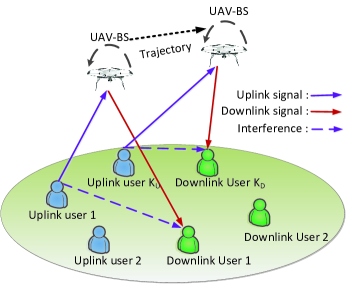
Figure 1: Full-duplex UAV aided small cell wireless systems

II System Model And Problem Formulation

We consider a UAV-enabled communication system where the UAV serves as a full-duplex BS that can communicate with $K_{D}$ single-antenna downlink users and $K_{U}$ single-antenna uplink users using the same and frequency resource as shown in Fig. 1. The UAV is equipped with two antennas, in which one is used for data transmission in the downlink and the other is used for data reception in the uplink. Define ${{\cal K}_{D}}{\rm{=}}\left\{{1,2,\ldots,{K_{D}}}\right\}$ and ${{\cal K}_{U}}{\rm{=}}\left\{{1,2,\ldots,{K_{U}}}\right\}$ as the sets of downlink and uplink users, respectively. We denote the horizontal coordinate of user $k$ as ${\bf w}_{k}$, $k\in{{\cal K}_{D}}\cup{{\cal K}_{U}}$. The UAV altitude is fixed at $H$. The given time period $T$ is equally divided into $N$ time slots with duration $\delta=T/N$. Then, the horizontal location of UAV at any slot $n$ is denoted as ${\bf q}[n]$.

As pointed out by the 3GPP, the UAV-ground channel model depends on the environmental scenarios, such as the suburban with less scattering and the macro urban with rich scattering. Especially when the UAV flies above $40\rm m$ in the rural area, the UAV offers a nearly 100% LoS probability for UAV-ground channel as shown in the 3GPP specification [10]. As a consequence, the downlink channel gain of UAV to the $j\text{-}\rm{th}$ downlink user at time slot $n$ is given by [11, 12, 9, 13]

$$h_{b,j}[n]={\beta_{0}}{\left({{{\left\|{{\bf{q}}\left[n\right]-{{\bf{w}}_{j}}}\right\|}^{2}}+{H^{2}}}\right)^{-1}},j\in{{\cal K}_{D}},$$ (1)

where $\beta_{0}$ represents the reference channel gain at $d=1{\rm m}$. Similarly, the uplink channel gain from the $i\text{-}\rm{th}$ uplink user to the UAV at time slot $n$ is denoted as $h_{i,b}[n]$, $i\in{{\cal K}_{U}}$.

The channel model from the $i\text{-}\rm{th}$ uplink user to the $j\text{-}\rm{th}$ downlink user follows Rayleigh fading with channel power gain denoted by ${g_{i,j}[n]}={\beta_{0}}d_{i,j}^{-\alpha}\xi$, where $d_{i,j}$ is the distance between the $i\text{-}\rm{th}$ uplink user and the $j\text{-}\rm{th}$ downlink user, $\alpha$ denotes the path loss exponent, and $\xi$ is a random variable following the exponential distribution with unit mean.

We adopt a TDMA manner for both downlink and uplink users, and assume that the UAV can only communicate with at most one user at one time slot in the uplink/downlink [4],[11], which yields the following user scheduling constraints

$$\sum\limits_{j=1}^{{K_{D}}}{x_{j}^{d}\left[n\right]}\leq 1,\forall n,$$ (2)

$$x_{j}^{d}\left[n\right]\in\left\{{0,1}\right\},\forall j,n,$$ (3)

$$\sum\limits_{i=1}^{{K_{U}}}{x_{i}^{u}\left[n\right]}\leq 1,\forall n,$$ (4)

$$x_{i}^{u}\left[n\right]\in\left\{{0,1}\right\},\forall i,n,$$ (5)

where (2)-(3) denote the downlink scheduling constraints, and (4)-(5) denote the uplink scheduling constraints.

The lower bound for the downlink ergodic capacity from the UAV to the $j\text{-}\rm{th}$ downlink user at time slot $n$ is given by

$$R_{j}^{d}\left[n\right]={\log_{2}}\left({1+\frac{{{p_{b}}{h_{b,j}}\left[n\right]}}{{\sum\limits_{i=1}^{{K_{U}}}{x_{i}^{u}\left[n\right]{\beta_{0}}d_{i,j}^{-\alpha}{p_{i}}\left[n\right]+{\sigma^{2}}}}}}\right),$$ (6)

where $\sigma^{2}$ denotes the noise power, and $p_{b}$ represents the UAV transmit power. Similarly, the uplink capacity from the $i\text{-}\rm{th}$ uplink user to the UAV is given by

$$R_{i}^{u}\left[n\right]={\log_{2}}\left({1+\frac{{{p_{i}}\left[n\right]{h_{i,b}}\left[n\right]}}{{{f_{b}}\left[n\right]+{\sigma^{2}}}}}\right),$$ (7)

where $f_{b}[n]$ denotes the self-interference at time slot $n$ from the transmit antenna to the receive antenna at the full-duplex UAV (Here, we assume that $f_{b}[n]$ is a constant to represent the maximal self-interference on the UAV [9]), and $p_{i}[n]$ denotes the $i\text{-}\rm{th}$ uplink user transmit power at time slot $n$.

Let ${{\bf{A}}_{\rm D}}=\left\{{x_{j}^{d}\left[n\right],\forall j,n}\right\},{{\bf{A}}_{\rm U}}=\left\{{x_{i}^{u}\left[n\right],\forall i,n}\right\},{\bf{P}}=\left\{{{p_{i}}\left[n\right],\forall i,n}\right\},{\bf{Q}}=\left\{{{\bf{q}}\left[n\right],\forall n}\right\}$. We aim at maximizing the total system capacity, including uplink and downlink links capacity, which is formulated as follows

$$\left({\rm{P}}\right) \mathop{\max}\limits_{{\bf{P}},{\bf{Q}},{{\bf{A}}_{\rm{D}}},{{\bf{A}}_{\rm{U}}}}\sum\limits_{n=1}^{N}{\sum\limits_{j=1}^{{K_{D}}}{x_{j}^{d}\left[n\right]}}R_{j}^{d}\left[n\right]+\sum\limits_{n=1}^{N}{\sum\limits_{i=1}^{{K_{U}}}{x_{i}^{u}\left[n\right]}}R_{i}^{u}\left[n\right]$$

$${\rm s.t.}~{}~{}0\leq{p_{i}}\left[n\right]\leq{P_{\max}},\forall i,n,$$ (8)

$$\quad\left\|{{\bf{q}}\left[n\right]-{\bf{q}}\left[{n-1}\right]}\right\|\leq{V_{\max}}\delta,\forall n,$$ (9)

$$\quad{{\bf{q}}_{I}}={\bf{q}}\left[0\right],{{\bf{q}}_{F}}={\bf{q}}\left[N\right],$$ (10)

$$\quad\eqref{const1},\eqref{const2},\eqref{const3},\eqref{const4},$$

where $P_{\rm max}$ and $V_{\rm max}$ respectively denote the maximum uplink user transmit power and UAV speed, ${\bf{q}}_{I}$ and ${\bf{q}}_{F}$ represent UAV’s initial and final location, respectively.

III Proposed Algorithm

The objective function is a function of $\bf Q$, $\bf P$, ${\bf A}_{\rm D}$, and ${\bf A}_{\rm U}$, which is not jointly convex with these variables. In addition, the binary constraints of (3) and (5) make the optimization more difficult to solve. The optimal solution is hard to obtain even using exhaustive search. First, the search space is ${\cal O}\left({{{\left({{K_{D}}{K_{U}}}\right)}^{N}}}\right)$ for solving downlink/uplink user scheduling, which means the complexity is exponentially increasing with the number of time slots $N$. Second, even with the fixed downlink and uplink user scheduling, the sub-problem is still non-convex with respective to uplink user transmit power and UAV trajectory, which indicates that the optimal solution still can not be obtained.

To deal with these issues, we first relax the binary variables ${\bf A}_{\rm D}$ and ${\bf A}_{\rm U}$ into continuous ones, and transform the binary constraints (3) and (5) into the linear constraints, which are respectively given by

$$0\leq x_{j}^{d}\left[n\right]\leq 1,\forall j,n,$$ (11)

$$0\leq x_{i}^{u}\left[n\right]\leq 1,\forall i,n.$$ (12)

Then, we propose a four-stage iterative optimization algorithm for solving problem $(\rm P)$, and a local solution is obtained.

III-A Stage 1: Downlink user scheduling design

First, we consider the downlink user scheduling problem with the given uplink user scheduling ${\bf A}_{\rm U}$, transmit power $\bf P$, and UAV trajectory $\bf Q$. Then, Problem $\rm P$ becomes the following optimization problem

$$\left({{\rm{P1}}}\right) \mathop{\max}\limits_{{{\bf{A}}_{\rm{D}}}}\sum\limits_{n=1}^{N}{\sum\limits_{j=1}^{{K_{D}}}{x_{j}^{d}\left[n\right]}}R_{j}^{d}\left[n\right]$$

$${\rm s.t.}~{}~{}\eqref{const2NEW}.$$

Obviously, problem $(\rm P1)$ is a standard linear programming problem, and can be efficiently solved by using standard optimization packages such as CVX.

III-B Stage 2: Uplink user scheduling design

Second, we study the uplink user scheduling problem with the given transmit power $\bf P$, downlink user scheduling ${\bf A}_{\rm D}$, and UAV trajectory $\bf Q$, which can be formulated as

$$\left({{\rm{P2}}}\right) \mathop{\max}\limits_{{{\bf{A}}_{\rm{U}}}}\sum\limits_{n=1}^{N}{\sum\limits_{j=1}^{{K_{D}}}{x_{j}^{d}\left[n\right]}}R_{j}^{d}\left[n\right]+\sum\limits_{n=1}^{N}{\sum\limits_{i=1}^{{K_{U}}}{x_{i}^{u}\left[n\right]}}R_{i}^{u}\left[n\right]$$

$${\rm s.t.}~{}~{}\eqref{const4NEW}.$$

The term $R_{j}^{d}\left[n\right]$ in objective function of problem $(\rm P2)$ is a strictly convex with respect to (w.r.t.) $x_{i}^{u}[n]$ and hence not concave. Hence, problem $(\rm P2)$ is a non-convex optimization problem. To deal with this issue, we approximate the convex function as its lower bound, which is linear function of the optimization variables that is much easier to solve. By taking the first-order Taylor expansion at any feasible point $\{x_{i}^{u,r}\}$, we have

$$R_{j}^{d}\left[n\right]\geq R_{j}^{d,lb}\left[n\right]\overset{\triangle}{=}{\log_{2}}\left({1+\frac{{{p_{b}}{h_{b,j}}\left[n\right]}}{{I_{j}^{r}\left[n\right]}}}\right)-$$

$$\quad\sum\limits_{i=1}^{{K_{U}}}{\frac{{{\beta_{0}}d_{i,j}^{-\alpha}{p_{i}}\left[n\right]{p_{b}}{h_{b,j}}\left[n\right]\log_{2}^{e}}}{{I_{j}^{r}\left[n\right]\left({I_{j}^{r}\left[n\right]+{p_{b}}{h_{b,j}}\left[n\right]}\right)}}\left({x_{i}^{u}\left[n\right]-x_{i}^{u,r}\left[n\right]}\right),}$$ (13)

where $I_{j}^{r}\left[n\right]=\sum\limits_{i=1}^{{K_{U}}}{x_{i}^{u,r}\left[n\right]{\beta_{0}}d_{i,j}^{-\alpha}{p_{i}}\left[n\right]+{\sigma^{2}}}$. As a result, for any given local point $\{{x_{i}^{u,r}}\}$, define the following problem

$$\left({{\rm{{\bar{P}}2}}}\right) \mathop{\max}\limits_{{{\bf{A}}_{\rm{U}}}}\sum\limits_{n=1}^{N}{\sum\limits_{j=1}^{{K_{D}}}{x_{j}^{d}\left[n\right]}}R_{j}^{d,lb}\left[n\right]+\sum\limits_{n=1}^{N}{\sum\limits_{i=1}^{{K_{U}}}{x_{i}^{u}\left[n\right]}}R_{i}^{u}\left[n\right]$$

$${\rm s.t.}~{}~{}\eqref{const4NEW}.$$

Now, problem $(\rm{\bar{P}}2)$ can be readily shown to be a convex optimization problem that can be efficiently solved. Then, $(\rm{P}2)$ can be approximately solved by successively updating the uplink user scheduling ${{{\bf{A}}_{\rm{U}}}}$ obtained from $(\rm{\bar{P}}2)$.

III-C Stage 3: UAV trajectory design

Third, we study the UAV trajectory optimization problem with the given transmit power $\bf P$, downlink user scheduling ${\bf A}_{\rm D}$, and uplink user scheduling ${\bf A}_{\rm U}$, which is given by

$$\left({{\rm{P3}}}\right) \mathop{\max}\limits_{\bf{Q}}\sum\limits_{n=1}^{N}{\sum\limits_{j=1}^{{K_{D}}}{x_{j}^{d}\left[n\right]}}R_{j}^{d}\left[n\right]+\sum\limits_{n=1}^{N}{\sum\limits_{i=1}^{{K_{U}}}{x_{i}^{u}\left[n\right]}}R_{i}^{u}\left[n\right]$$

$${\rm s.t.}~{}~{}\eqref{const6},\eqref{const7}.$$

Problem $(\rm{P}3)$ is a non-convex optimization problem since the objective function is non-convex. To handle the non-convex objective function, the successive convex approximation technique is applied. It can be observed that $R_{j}^{d}\left[n\right]$ is convex w.r.t. ${\left\|{{\bf{q}}\left[n\right]-{{\bf{w}}_{j}}}\right\|^{2}}$, but it is not convex w.r.t. ${\bf q}[n]$. By taking the first-order Taylor expansion at any given local point ${\left\|{{{\bf{q}}^{r}}\left[n\right]-{{\bf{w}}_{i}}}\right\|^{2}}$, we can obtain its convex lower bound as follows

$$R_{j}^{d}\left[n\right]\geq{\log_{2}}\left({1+\frac{{{C_{j}}\left[n\right]}}{{{{\left\|{{{\bf{q}}^{r}}\left[n\right]-{{\bf{w}}_{j}}}\right\|}^{2}}+{H^{2}}}}}\right)-{\Sigma_{j}}\left[n\right]\times$$

$$\left({{{\left\|{{\bf{q}}\left[n\right]-{{\bf{w}}_{j}}}\right\|}^{2}}-{{\left\|{{{\bf{q}}^{r}}\left[n\right]-{{\bf{w}}_{j}}}\right\|}^{2}}}\right)\overset{\triangle}{=}{\psi^{lb}}\left({R_{j}^{d}\left[n\right]}\right),$$ (14)

where ${\Sigma_{j}}\left[n\right]=\frac{{{C_{j}}\left[n\right]\log_{2}^{e}}}{{\left({{C_{j}}\left[n\right]+{{\left\|{{{\bf{q}}^{r}}\left[n\right]-{{\bf{w}}_{j}}}\right\|}^{2}}+{H^{2}}}\right)\left({{{\left\|{{{\bf{q}}^{r}}\left[n\right]-{{\bf{w}}_{j}}}\right\|}^{2}}+{H^{2}}}\right)}}$ and ${C_{j}}\left[n\right]=\frac{{{p_{b}}{\beta_{0}}}}{{\sum\limits_{i=1}^{{K_{U}}}{x_{i}^{u}\left[n\right]{\beta_{0}}d_{i,j}^{-\alpha}{p_{i}}\left[n\right]+{\sigma^{2}}}}}$. Similarly, to tackle the non-convexity of $R_{i}^{u}\left[n\right]$, for any given local point ${\left\|{{{\bf{q}}^{r}}\left[n\right]-{{\bf{w}}_{i}}}\right\|^{2}}$, we have

$$R_{i}^{u}\left[n\right]\geq{\log_{2}}\left({1+\frac{{{E_{i}}\left[n\right]}}{{{{\left\|{{{\bf{q}}^{r}}\left[n\right]-{{\bf{w}}_{i}}}\right\|}^{2}}+{H^{2}}}}}\right)-{F_{i}}\left[n\right]\times$$

$$\left({{{\left\|{{\bf{q}}\left[n\right]-{{\bf{w}}_{i}}}\right\|}^{2}}-{{\left\|{{{\bf{q}}^{r}}\left[n\right]-{{\bf{w}}_{i}}}\right\|}^{2}}}\right)\overset{\triangle}{=}{\varphi^{lb}}\left({R_{i}^{u}\left[n\right]}\right),$$ (15)

where ${F_{i}}\left[n\right]=\frac{{\log_{2}^{e}}{E_{i}[n]}}{{\left({{E_{i}}\left[n\right]+{{\left\|{{{\bf{q}}^{r}}\left[n\right]-{{\bf{w}}_{i}}}\right\|}^{2}}+{H^{2}}}\right)\left({{{\left\|{{{\bf{q}}^{r}}\left[n\right]-{{\bf{w}}_{i}}}\right\|}^{2}}+{H^{2}}}\right)}}$ and ${E_{i}}\left[n\right]=\frac{{{p_{i}}\left[n\right]{\beta_{0}}}}{{{f_{b}}\left[n\right]+{\sigma^{2}}}}$. As a result, with (14) and (15), problem $(\rm{P}3)$ can be simplified as

$$\left({{\rm{\bar{P}3}}}\right)\mathop{\max}\limits_{\bf{Q}}\sum\limits_{n=1}^{N}{\sum\limits_{j=1}^{{K_{D}}}{x_{j}^{d}\left[n\right]}}{\psi^{lb}}\left({R_{j}^{d}\left[n\right]}\right)+$$

$$\qquad\qquad\qquad\qquad\qquad\qquad\sum\limits_{n=1}^{N}{\sum\limits_{i=1}^{{K_{U}}}{x_{i}^{u}\left[n\right]}}{\varphi^{lb}}\left({R_{i}^{u}\left[n\right]}\right)$$

$${\rm s.t.}~{}~{}\eqref{const6},\eqref{const7}.$$

Problem $(\rm{\bar{P}}3)$ is now a convex optimization problem. Then, we can obtain the locally optimal solution of $(\rm{P}3)$ by iteratively solving problem $(\rm{\bar{P}}3)$ to update the UAV trajectory.

III-D Stage 4: Uplink user transmit power control

Finally, we study the uplink user transmit power optimization problem with the given UAV trajectory $\bf Q$, downlink user scheduling ${\bf A}_{\rm D}$, and uplink user scheduling ${\bf A}_{\rm U}$, which is given by

$$\left({{\rm{P4}}}\right) \mathop{\max}\limits_{\bf{P}}\sum\limits_{n=1}^{N}{\sum\limits_{j=1}^{{K_{D}}}{x_{j}^{d}\left[n\right]}}R_{j}^{d}\left[n\right]+\sum\limits_{n=1}^{N}{\sum\limits_{i=1}^{{K_{U}}}{x_{i}^{u}\left[n\right]}}R_{i}^{u}\left[n\right]$$

$${\rm s.t.}~{}~{}\eqref{const5}.$$

The term $R_{j}^{d}\left[n\right]$ is convex w.r.t. $p_{i}[n]$ which makes problem ${(\rm P}4)$ be a non-convex optimization problem. Similar to that of $(\rm{\bar{P}}2)$, by taking the first-order Taylor expansion at local point $\{p_{i}^{r}[n]\}$, we can approximate it as its lower bound as follows

$$R_{j}^{d}\left[n\right]\geq{\phi^{lb}}\left({R_{j}^{d}\left[n\right]}\right)\overset{\triangle}{=}{\log_{2}}\left({1+\frac{{{p_{b}}{h_{b,j}}\left[n\right]}}{{G_{j}^{r}\left[n\right]}}}\right)-$$

$$\qquad\sum\limits_{i=1}^{{K_{U}}}{\frac{{{\beta_{0}}x_{i}^{u}\left[n\right]d_{i,j}^{-\alpha}{p_{b}}{h_{b,j}}\left[n\right]\log_{2}^{e}}}{{G_{j}^{r}\left[n\right]\left({G_{j}^{r}\left[n\right]+{p_{b}}{h_{b,j}}\left[n\right]}\right)}}\left({{p_{i}}\left[n\right]-p_{i}^{r}\left[n\right]}\right)},$$ (16)

where $G_{j}^{r}\left[n\right]=\sum\limits_{i=1}^{{K_{U}}}{x_{i}^{u}\left[n\right]{\beta_{0}}d_{i,j}^{-\alpha}p_{i}^{r}\left[n\right]+{\sigma^{2}}}$. Then, with (16), problem $(\rm{P}4)$ is simplified as

$$\left({{\rm{\bar{P}4}}}\right) \mathop{\max}\limits_{\bf{P}}\sum\limits_{n=1}^{N}{\sum\limits_{j=1}^{{K_{D}}}{x_{j}^{d}\left[n\right]}}{\phi^{lb}}\left({R_{j}^{d}\left[n\right]}\right)+\sum\limits_{n=1}^{N}{\sum\limits_{i=1}^{{K_{U}}}{x_{i}^{u}\left[n\right]}}R_{i}^{u}\left[n\right]$$

$${\rm s.t.}~{}~{}\eqref{const5}.$$

Problem $(\rm{\bar{P}}4)$ is a convex optimization problem. Then, $(\rm{P}4)$ can be approximately solved by successively updating the uplink user transmit power obtained from problem $(\rm{\bar{P}}4)$.

III-E Overall algorithm

Based on the above four-stage sub-problems, we optimize the four-stage sub-problems in an iterative way, which is summarized in Algorithm 1. Note that Algorithm 1 is guaranteed to converge a local solution, which can be found in [4],[9]. At last, the continuous user scheduling variable is reconstructed into binary one by adopting the following simple criteria [11]: $x=\left\{\begin{array}[]{l}1,\;\;\;{\rm{if}}\;\;x\geq 0.5,\\ 0,\;\;\;{\rm{if}}\;\;x<0.5,\end{array}\right.$ where $x\in\left\{{x_{i}^{u}\left[n\right],x_{j}^{d}\left[n\right],\forall i,j,n}\right\}$.

Algorithm 1 Alternating optimization for problem $(\rm P)$

1:  Initialize ${{\bf{q}}^{r}[n]}$, $x_{i}^{u,r}[n]$, $p_{i}^{r}[n]$, and set $r\leftarrow 0$ as well as tolerance $\epsilon>0$.

2:  repeat.

3:   Solve $(\rm P1)$ for given $\{{\bf q}^{r}[n],x_{i}^{u,r}[n],p_{i}^{r}[n]\}$, and  denote the optimal solution as $\{{x_{j}^{d,r+1}\left[n\right]}\}$.

4:   Solve $(\rm P2)$ for given $\{{\bf q}^{r}[n],{x_{j}^{d,r+1}\left[n\right]},p_{i}^{r}[n]\}$, and  denote the optimal solution as $\{x_{i}^{u,r+1}[n]\}$.

5:   Solve $(\rm P3)$ for given $\{x_{i}^{u,r+1}[n],{x_{j}^{d,r+1}\left[n\right]},p_{i}^{r}[n]\}$, and  denote the optimal solution as $\{{\bf q}^{r+1}[n]\}$.

6:   Solve $(\rm P4)$ for given $\{x_{i}^{u,r+1}[n],{x_{j}^{d,r+1}\left[n\right]},{\bf q}^{r+1}[n]\}$, and denote the optimal solution as $\{p_{i}^{r+1}[n]\}$.

7:   $r\leftarrow r+1$.

8:  until the fractional increase of the objective value of $\left({{\rm{P}}}\right)$ is less than tolerance $\epsilon$.

It is worth pointing out that all the sub-problems $\rm(P1)$, $\rm(\bar{P}2)$, $\rm(\bar{P}3)$, and $\rm(\bar{P}4)$ are convex, thus the computational complexity of Algorithm is ${\cal O}\Big{(}{{L_{4}}}\left({{{\left({{K_{D}}N}\right)}^{3.5}}+{L_{1}}{{\left({{K_{U}}N}\right)}^{3.5}}+{L_{2}}{{\left({2N}\right)}^{3.5}}+}\right.$ $\left.{\left.{{L_{3}}{{\left({{K_{U}}N}\right)}^{3.5}}}\right)}\right)$ with $L_{1}$, $L_{2}$, $L_{3}$, and $L_{4}$ being the iterative numbers.

IV Simulation Results

Fig. 2 UAV trajectory for different period $T$.

Fig. 3 Uplink user transmit power.

In this section, we evaluate the performance of full-duplex UAV system by our proposed algorithm. In our example, we consider four downlink users and four uplink users, i.e., $K_{D}=4$ and $K_{U}=4$. The channel gain of the system and noise power are respectively set as ${\beta_{0}}=-60{\rm{dB}}$ and $\sigma^{2}=-110{\rm dBm}$ [4]. The system bandwidth is assumed to be $B=1{\rm MHz}$. The UAV maximum transmit power and speed are respectively assumed to be $p_{b}=0.1{\rm W}$ and $V_{\rm max}=50{\rm{m/s}}$ [12]. We set $\alpha=3$, $\delta=0.5s$, $P_{\rm max}=0.1{\rm W}$. Unless otherwise specified, we set ${H=100\rm{m}}$ and $f_{b}[n]=-130{\rm dB}$, $\epsilon=10^{-3}$.

Fig. 2 shows the obtained UAV trajectories by our proposed Algorithm for three different periods, i.e., $T=30s$, $T=50s$, and $T=150s$. The UAV’s initial and final location are ${\bf q}_{I}=\left({0,500{\rm m}}\right)^{T}$ and ${\bf q}_{F}=\left({1000{\rm m},500{\rm m}}\right)^{T}$, respectively. The circle and square represent locations of uplink and downlink users, respectively. $D_{i}$ and $U_{i}$ denotes the $i$-th downlink and uplink user, respectively. It is observed that the UAV prefers moving closer to the downlink users rather than the uplink users for all the three different periods. The reason is that the downlink users are exposed to the strong interference from the uplink users, and the UAV moving closer to the downlink users can enlarge the downlink capacity. To illustrate it clearly, the uplink user transmit power for $T=50s$ is plotted in Fig. 3. We can observe from this figure that for the proximity of two uplink users, one transmits with the maximal power and the other transmits with a lower power in order to reduce the interference to the nearby downlink users.

Fig. 4 Self-interference versus capacity.

Fig. 5 UAV altitude versus capacity.

In Fig. 4, we investigate the impact of self-interference on the sum of system capacity for period $T=70s$. It is observed that the sum of capacity is monotonically non-increasing with the self-interference. Especially, when the power of self-interference $f_{b}[n]$ below $-150\rm dB$, the sum of capacity is not be changed. This is because the power level of self-interference is much smaller than the noise power, i.e., $\sigma^{2}=-110{\rm dBm}$, thus the impact of self-interference on the system can be neglected. However, when the power of self-interference $f_{b}[n]$ exceeds $-150\rm dB$, the power of interference can not be ignored compared to the noise power, which results in a poor system performance.

In Fig. 5, the effect of UAV altitude on the system performance is studied. It is observed that the system performance is significantly decreasing with the UAV altitude. This is expected since the higher UAV altitude resulting in a lower signal-to-noise (SNR) for uplink and downlink. This result can also be directly seen in expressions (6) and (7).

In Fig. 6, we compare our proposed design with the following benchmarks: 1) Ideal no interference: in this scheme when calculating the objective function value, we ignore the interference from the uplink users to the downlink users. Hence, this scheme can serve as the performance upper bound. 2) Proposed design: we jointly optimize the UAV trajectory, downlink/uplink user scheduling, and uplink transmit power. 3) No power control scheme: we assume that the uplink users transmit with the maximal power, and other variables are still optimized. 4) Straight flight scheme: the UAV flies in a straight line from ${\bf q}_{I}$ to ${\bf q}_{F}$ with constant speed $\frac{{\left\|{{{\bf{q}}_{F}}-{{\bf{q}}_{I}}}\right\|}}{T}$. 5) Static scheme: UAV stays at a position with a fixed UAV altitude $H$ that minimizes the sum of distance to all the users, i.e., the horizontal UAV location is calculated from ${\bf{q}}_{static}^{opt}=\mathop{\min}\limits_{{{\bf{q}}_{static}}}\sum\limits_{i=1}^{{{\cal K}_{U}}\cup{{\cal K}_{D}}}{{{\left\|{{{\bf{q}}_{static}}-{{\bf{w}}_{i}}}\right\|}^{2}}}$. 6) Half-duplex scheme (HD): UAV operates in a half-duplex mode, the interference imposed on the downlink users is disappeared. Note that each time slot is further divided into two time sub-slots with the same duration ${\delta\mathord{\left/{\vphantom{\delta 2}}\right.\kern-1.2pt}2}$, and at each time slot, one time sub-slot is assigned to uplink users and the other is assigned to uplink users. In addition, for straight flight and static benchmarks, the downlink/uplink user scheduling and uplink user transmit power are still optimized. Several insights can be made from Fig. 6. First, we can observe that the interference from the uplink users to the downlink users severely deteriorates the system capacity. Second, the system capacity can be prominently improved by designing the UAV trajectory. Third, the half-duplex UAV performs worst over other benchmarks. This result shows that with the help of full-duplex technique, it provides much system performance gain compared to the half-duplex technique. At last, we find that the system capacity gain of our proposed algorithm over the power control scheme is marginal. This is because that the downlink capacity can be improved by reducing the uplink user transmit power while the uplink capacity will be decreased. Therefore, the sum of downlink and uplink capacity will not improve too much. However, if we consider a fairness metric over the users, we will show that the uplink user transmit power will significantly impact on the system performance in the next figure .

Fig. 6 Sum of capacity versus $T$.

Fig. 7 Max-min rate versus period $T$.

In Fig. 7, the benchmarks are the same for that of Fig. 6, but the goal of this design is to maximize the minimum average capacity over both uplink users and downlink users for a fair consideration. Similar results can be obtained from that of Fig. 6 except for the last insight. It is observed from Fig. 7 that the proposed scheme with uplink user power control significantly outperforms no power control scheme in terms of achievable rate. This is because for achieving a fairness of system performance over the uplink and downlink users, the uplink user transmit should be carefully optimized.

V Conclusion

This paper studied the UAV acted as a full-duplex base station to serve the ground users. We formulated a sum of uplink and downlink throughput maximization problem by alternately optimizing the UAV trajectory, downlink/uplink user scheduling, and uplink user transmit power. To address the resulting optimization problem, we developed an efficient iterative algorithm to solve it. The simulation results showed that a significant performance gain is improved compared to that of half-duplex UAV. In addition, the results also showed that the system performance was prominently improved by optimizing the uplink user transmit power as well as UAV trajectory in terms of average capacity.

References

• [1] C. Zhan, Y. Zeng, and R. Zhang, “Energy-efficient data collection in UAV enabled wireless sensor network,” IEEE Wireless Communications Letters, vol. 7, no. 3, pp. 328–331, 2018.
• [2] J. Xu, Y. Zeng, and R. Zhang, “UAV-enabled wireless power transfer: Trajectory design and energy optimization,” IEEE Transactions on Wireless Communications, vol. 17, no. 8, pp. 5092–5106, 2018.
• [3] J. Lyu, Y. Zeng, and R. Zhang, “UAV-aided offloading for cellular hotspot,” IEEE Transactions on Wireless Communications, vol. 17, no. 6, pp. 3988–4001, 2018.
• [4] Q. Wu, Y. Zeng, and R. Zhang, “Joint trajectory and communication design for multi-UAV enabled wireless networks,” IEEE Transactions on Wireless Communications, vol. 17, no. 3, pp. 2109–2121, 2018.
• [5] Y. Sun, D. Xu, D. W. K. Ng, L. Dai, and R. Schober, “Optimal 3D-trajectory design and resource allocation for solar-powered UAV communication systems,” IEEE Transactions on Communications, vol. 67, no. 6, pp. 4281–4298, 2019.
• [6] S. Zhang, H. Zhang, Q. He, K. Bian, and L. Song, “Joint trajectory and power optimization for UAV relay networks,” IEEE Communications Letters, vol. 22, no. 1, pp. 161–164, 2018.
• [7] J. I. Choi, M. Jain, K. Srinivasan, P. Levis, and S. Katti, “Achieving single channel, full duplex wireless communication,” in Proceedings of the sixteenth annual international conference on Mobile computing and networking.   ACM, 2010, pp. 1–12.
• [8] M. Hua, Y. Wang, Z. Zhang, C. Li, Y. Huang, and L. Yang, “Outage probability minimization for low-altitude UAV-enabled full-duplex mobile relaying systems,” China Communications, vol. 15, no. 5, pp. 9–24, 2018.
• [9] H. Wang, J. Wang, G. Ding, J. Chen, Y. Li, and Z. Han, “Spectrum sharing planning for full-duplex UAV relaying systems with underlaid D2D communications,” IEEE Journal on Selected Areas in Communications, vol. 36, no. 9, pp. 1986–1999, 2018.
• [10] 3GPP, “Enhanced LTE support for aerial vehicles,” accessed on Nov. 1, 2019, [Online] Available: https://portal.3gpp.org/ngppapp/CreateTdoc.aspx?mode=view&contributionUid=RP-172779.
• [11] M. Hua, Y. Wang, Z. Zhang, C. Li, Y. Huang, and L. Yang, “Power-efficient communication in UAV-aided wireless sensor networks,” IEEE Communications Letters, vol. 22, no. 6, pp. 1264–1267, 2018.
• [12] Y. Zeng and R. Zhang, “Energy-efficient UAV communication with trajectory optimization,” IEEE Transactions on Wireless Communications, vol. 16, no. 6, pp. 3747–3760, 2017.
• [13] B. Duo, Q. Wu, X. Yuan, and R. Zhang, “Energy efficiency maximization for full-duplex UAV secrecy communication,” arXiv preprint arXiv:1906.07346, 2019.