Error analysis of mixed THz-RF wireless systems

Abstract

In this letter, we introduce a novel mixed terahertz (THz)-radio frequency (RF) wireless system architecture, which can be used for backhaul/fronthaul applications, and we deliver the theoretical framework for its performance assessment. In more detail, after identifying the main design parameters and characteristics, we derive novel closed-form expressions for the end-to-end signal-to-noise ratio cumulative density function, the outage probability and the symbol error rate, assuming that the system experiences the joint effect of fading and stochastic antenna misalignment. The derived analytical framework is verified through simulations and quantifies the system’s effectiveness and reliability. Finally, our results contribute to the extraction of useful design guidelines.

I Introduction

Terahertz (THz) wireless systems have become a topic of much hype both in academia and industry, due to the high spectrum availability that they offer [1, 2, 3]. In addition, they are license-free; hence, they are cost-effective relative to the radio frequency (RF) ones. Therefore, THz wireless systems are expected to become attractive backhaul solutions. On the other hand, they have considerably high sensitivity to blockage; especially, in urban environment with high obstacles density. Thus, their usage in fronthaul scenarios is questionable. This observation aspires the investigation of mixed THz-radio frequency (RF) wireless systems as promising backhaul-fronthaul solutions. This concept is envisioned to allow multiple RF links to feed one THz link. Such a use case may be employed in harsh environments, where the fiber optic structure is under development in order to increase the installation flexibility and last mile quality of experience.

Scanning the technical literature, a great amount of research effort has been put on modeling and evaluating the performance of both THz [4, 5, 6, 7, 8, 9, 10, 11] and RF wireless systems (see e.g., [12] and references therein). In particular, in [4], the authors reported a novel THz-band propagation model, whereas, in [5], a simplified molecular absorption loss model was delivered. The latter model was used in [6] for the quantification of the THz link capacity. The con of the above mentioned contributions is that they overestimated the THz system performance, since they neglect the impact of fading, which can be generated due to scattering on aerosols [7]. On the contrary, in [8] and [9], the authors modeled fading as stochastic processes. In particular, in [8], they experimentally proved that the envelope of the fading coefficient follows Nakagami-m distribution under both non-line-of-sight and line-of-sight conditions. Similarly, in [9], the authors delivered experimental verifications of the existence of shadowing in the $300\text{ }\mathrm{GHz}$ band. Likewise, in [10], the impact of antenna misalignment was investigated, while, in [11], the joint impact of antenna misalignment and fading in THz wireless systems was evaluated in terms of outage probability (OP) and capacity. On the other hand, the performance of relaying systems operating in the RF band have been studied in several works (see e.g.,[13, 14, 15] and references therein). The aforementioned contributions assumed that the links at both hops operate in the same frequency band; hence, the same fading distribution was assumed for both of them. However, this is not a valid assumption for links, which are established in different bands.

To the best of the authors knowledge, despite their paramount importance, mixed THz-RF wireless systems have not been proposed and their performance has not been studied. Motivated by this, in this letter, we introduce the mixed THz-RF wireless system architecture, we present the theoretical framework that quantifies its outage as well as error performance and provides useful design guidelines. In more detail, we report the system model that take into consideration the main design parameters as well as both the THz and RF channels particularities. In this direction, it is worth-noting that the fading coefficient envelope of the THz channel, in this work, is modeled as an $\alpha-\mu$ distribution. This distribution is configurable and can be simplified into Rayleigh, Nakagami-$m$ as well as Gamma in order to accommodate both the impact of multipath fading and shadowing. Moreover, in order to incorporate the effect of antenna misalignment, we modeled the elevation and horizontal displacement at the THz receiver plane as independent and identical Gaussian distributions. Building upon the system and channel models, we derive novel exact closed-form expressions for the cumulative density function (CDF) of the end-to-end (e2e) SNR, the OP and symbol error rate (SER). These expressions are verified through respective simulations and can be used to accurately evaluate the mixed THz-RF wireless system performance.

Notations

The absolute value and exponential function are denoted by $|\cdot|$, and $\exp\left(x\right)$, respectively. Likewise, $\sqrt{x}$ returns the square root of $x$ and $\min\left(\cdot,\cdot\right)$ represented the minimum operator. Moreover, $P_{r}\left(\mathcal{A}\right)$ is the probability that the event $\mathcal{A}$ is valid. The upper incomplete Gamma [16, eq. (8.350/2)] and Gamma [16, eq. (8.310)] functions are respectively denoted by $\Gamma\left(\cdot,\cdot\right)$, and $\Gamma\left(\cdot\right)$, while the Q-function is reprented by $Q\left(\cdot\right)$ [17]. Finally, $G_{p,q}^{m,n}\left(x\left|\begin{array}[]{c}a_{1},a_{2},\cdots,a_{p}\\ b_{1},b_{2},\cdots,b_{q}\end{array}\right.\right)$ returns the Meijer G-function [16, eq. (9.301)], and $H_{p,q}^{m,n}\left[z\left|\begin{array}[]{c}(a_{1},b_{1}),\cdots,(a_{p},b_{p})\\ (c_{1},d_{1}),\cdots,(c_{p},d_{p})\end{array}\right.\right]$ stands for the Fox H-function [18, eq. (8.3.1/1)].

II System model

We consider a mixed THz-RF dual-hop decode-and-forward (DF) system that is used for downlink. The direct link between the source (S) and destination (D) is assumed to be weak enough to be ignored. Moreover, a relay (R) is employed, which is equipped with a THz receiver and an RF transmitter. We assume that the S-R link is established in the THz band, whereas the R-D link is utilized in the RF band. Likewise, it is assumed that R operates in half-duplex mode. Thus, in the first timeslot, R listens to S, whereas in the second timeslot, R, decodes, re-encodes and forwards to D the received signal.

II-A THz link

The received signal at R can be expressed as

$$y_{r}=h_{r}s+w_{r},$$ (1)

where $s$ and $w_{r}$ are respectively the signal transmitted by S and the zero-mean additive white Gaussian noise (AWGN), with variance $N_{o,1}$. Additionally, $h_{r}$ represents the THz channel coefficient that can be analyzed as

$$h_{r}=h_{l}h_{pf}.$$ (2)

In (2), $h_{l}$ is the deterministic path-gain and can be obtained, according to [11, eqs. (5)-(17)], as

$$h_{l}=\frac{c\sqrt{G_{t,1}G_{r,1}}}{4\pi f_{1}d_{1}}\exp\left(-\frac{1}{2}\kappa(f_{1},T,\psi,p)d_{1}\right),$$ (3)

where $c$, $f_{1}$, and $d_{1}$ respectively denote the speed of light, the transmission frequency, and distance, while $G_{t,1}$, and $G_{r,1}$ are the THz transmission and reception antenna gains. Likewise, $\kappa(f_{1},T,\psi,p)$ is the molecular absorption coefficient, depends on the temperature, $T$, the relative humidity, $\psi$, as well as the atmospheric pressure, $p$, and can be calculated as

$$\kappa(f_{1},T,\psi,p) =\frac{q_{1}v(q_{2}v+q_{3})}{(q_{4}v+q_{5})^{2}+\left(\frac{f_{1}}{100c}-p_{1}\right)^{2}}$$

$$+\frac{q_{6}v(q_{7}v+q_{8})}{(q_{9}v+q_{10})^{2}+\left(\frac{f_{1}}{100c}-p_{2}\right)^{2}}$$

$$+c_{1}f_{1}^{3}+c_{2}f_{1}^{2}+c_{3}f+c_{4},$$ (4)

with $q_{1}=0.2205$, $q_{2}=0.1303$, $q_{3}=0.0294$, $q_{4}=0.4093$, $q_{5}=0.0925$, $q_{6}=2.014$, $q_{7}=0.1702$, $q_{8}=0.0303$, $q_{9}=0.537$, $q_{10}=0.0956$, $c_{1}=5.54\times 10^{-37}\text{ }\mathrm{Hz}^{-3}$, $c_{2}=-3.94\times 10^{-25}\text{ }\mathrm{Hz}^{-2}$, $c_{3}=9.06\times 10^{-14}\text{ }\mathrm{Hz}^{-1}$, $c_{4}=-6.36\times 10^{-3}\text{ }\mathrm{Hz}^{-3}$, $p_{1}=10.835\text{ }\mathrm{cm}^{-1}$, $p_{2}=12.664\text{ }\mathrm{cm}^{-1}$, $v=\frac{\psi}{100}\frac{p_{w}(T,p)}{p}$, and $p_{w}(T,p)$ is the saturated water vapor partial pressure in temperature T, which can be evaluated based on Buck’s equation.

Moreover, $h_{pf}$ is a random variable that accommodates the joint impact of fading and antenna misalignment, with probability density function (PDF) and CDF that can be respectively expressed as [11, eqs. (26), and (27)]

$$f_{|h_{fp}|}(x)=\phi S_{0}^{-\phi} \frac{\mu^{\frac{\phi}{\alpha}}}{\hat{h}_{f}^{\alpha}\Gamma\left(\mu\right)}x^{\phi-1}$$

$$\times\Gamma\left(\frac{\alpha\mu-\phi}{\alpha},\mu\frac{x^{\alpha}}{\hat{h}_{f}^{\alpha}}S_{0}^{-\alpha}\right).$$ (5)

and

$$F_{|h_{fp}|}(x) =1-\frac{1}{\alpha}\frac{x^{\phi}}{\hat{h}_{f}^{\phi}}\frac{\phi}{S_{0}^{\phi}}$$

$$\times\sum_{k=0}^{\mu-1}\frac{\mu^{\frac{\phi}{\alpha}}}{k!}\Gamma\left(\frac{\alpha k-\phi}{\alpha},{\mu\frac{x^{\alpha}}{\hat{h}_{f}^{\alpha}}}S_{0}^{-\alpha}\right),$$ (6)

where $\alpha>0$ is the distribution parameter and $\mu$ is the normalized variance of the fading channel envelope that follows $\alpha-\mu$ distribution, $\hat{h}_{f}$ is the $\alpha$-root mean value of the fading channel envelope, $S_{0}$ is the fraction of the collected power when the transceivers antennas are fully-aligned and can be evaluated as $S_{0}=\left|\operatorname{erf}\left(\zeta\right)\right|^{2},$ with $\zeta=\sqrt{\frac{\pi}{2}}\frac{r_{1}}{w_{d1}}$, $r_{1}$ and $w_{d1}$ respectively representing the radius of the reception antenna effective area and the transmission beam footprint radius at distance $d_{1}$. Additionally, $\phi$ is the squared ratio of the equivalent beam width radius at R, $w_{e}$, to the doubled spatial jitter standard deviation, $\sigma_{s}$, and can be defined as $\phi=\frac{w_{e}^{2}}{2\sigma_{s}^{2}}$, where $w_{e}^{2}=w_{d1}^{2}\frac{\sqrt{\pi}\operatorname{erf}(\zeta)}{2\zeta\exp(-\zeta^{2})}$.

II-B RF link

The received signal at D is given by

$$y_{2}=h_{2}\tilde{s}+w_{2},$$ (7)

where $\tilde{s}$, $h_{2}$ and $w_{2}$ denote respectively the R transmitted signal, the RF channel coefficient and the zero-mean AWGN with variance $N_{o,2}$. The channel coefficient of the RF link, $h_{2}$, can be expressed as $h_{2}=h_{g}h_{f},$ where $h_{g}$ stands for the deterministic path-gain and can be obtained as $h_{g}=\xi d_{2}^{-\eta_{2}/2}$, with $\xi$, $\eta_{2}$, and $d_{2}$ respectively being the deterministic path-gain coefficient, the RF link path-loss exponent, and the R-D distance, while $h_{f}$ denotes the fading channel coefficient. We assume that the envelope of $h_{f}$ follows Rayleigh distribution. Note that in urban environments, there are several objects that scatter the radio signal, before it arrives at the RX; hence, Rayleigh is a reasonable model for the RF link.

III Performance analysis

III-A End-to-end SNR statistics

The e2e SNR of the mixed THz-RF wireless system can be expressed as

$$\gamma_{e}=\min\left(\gamma_{1},\gamma_{2}\right),$$ (8)

where

$$\gamma_{1}=\frac{\left|h_{l}\right|^{2}\left|h_{pf}\right|^{2}E_{s}}{N_{o,1}}\text{ and }\gamma_{2}=\frac{\left|h_{g}\right|^{2}\left|h_{f}\right|^{2}E_{r}}{N_{o,2}},$$ (9)

with $E_{s}$ and $E_{r}$ denoting the S and R transmission powers, respectively.

The following theorem returns an insightful closed-form expression for the CDF of the e2e SNR of the mixed THz-RF link.

Theorem 1.

The CDF of the e2e SNR of the mixed THz-RF link can be obtained as in (10), given at the top of the next page.

$$F_{\gamma_{e}}\left(x\right)=1-\frac{\phi}{\alpha}\left(\frac{N_{o,1}}{S_{0}^{2}\hat{h}_{f}^{2}\left|h_{l}\right|^{2}E_{s}}\right)^{\phi/2}\sum_{k=0}^{\mu-1}\frac{\mu^{\frac{\phi}{\alpha}}}{k!}x^{\phi/2}\exp{\left(-\frac{N_{o,2}x}{|h_{g}|^{2}E_{r}}\right)}\Gamma\left(\frac{\alpha k-\phi}{\alpha},{\mu\left(\frac{N_{o,1}}{\left|h_{l}\right|^{2}E_{s}}\right)^{\alpha/2}\frac{x^{\alpha/2}}{\hat{h}_{f}^{\alpha}S_{0}^{\alpha}}}\right)$$ (10)

Proof:

Please refer to Appendix A. ∎

Remark 1. From (10), the OP can be evaluated as $P_{o}\left(\gamma_{th}\right)=F_{\gamma_{e}}\left(\gamma_{th}\right),$ where $\gamma_{th}$ is the SNR threshold.

III-B Average SER

The following theorem returns a closed-form expression for the average SER.

Theorem 2.

The average SER of the mixed THz-RF wireless system can be analytically evaluated as in (13), given at the top of the next page.

$$\overline{P}_{e} =\frac{a}{2}-a\sqrt{\frac{b}{4\pi}}\frac{\phi\mu^{\frac{\phi}{\alpha}}}{\alpha}\left(\frac{N_{o,1}}{S_{0}^{2}\hat{h}_{f}^{2}\left|h_{l}\right|^{2}E_{s}}\right)^{\phi/2}\left(\frac{N_{o,2}}{|h_{g}|^{2}E_{r}}+b\right)^{-\frac{\phi+1}{2}}$$

$$\times\sum_{k=0}^{\mu-1}\frac{1}{k!}H_{3,3}^{2,2}\left(\frac{\mu\left(\frac{N_{o,1}}{\left|h_{l}\right|^{2}E_{s}}\right)^{\alpha/2}\frac{1}{\hat{h}_{f}^{\alpha}S_{0}^{\alpha}}}{\left(\frac{N_{o,2}}{|h_{g}|^{2}E_{r}}+b\right)^{\alpha/2}}\left|\begin{array}[]{c}\left(-\frac{\phi+1}{2},\frac{\alpha}{2}\right),\left(\frac{1-\phi}{2},\frac{\alpha}{2}\right),\left(1,1\right)\\ \left(\frac{\alpha k-\phi}{\alpha},1\right),\left(0,1\right),\left(-\frac{\phi+1}{2},\frac{\alpha}{2}\right)\end{array}\right.\right)$$ (13)

In (13), $a$ and $b$ are modulation-specific constants (e.g., binary shift keying (BPSK): $a=1$ and $b=0.5$, quadrature phase shift keying (QPSK) $a=1$ and $b=0.25$, and $M-$ quadrature amplitude modulation (QAM): $a=4$ and $b=\frac{3}{M-1}$).

Proof:

Please refer to Appendix B. ∎

IV Results & Discussion

In this section, we illustrate the outage and error performance of the mixed THz-RF wireless system by providing analytical and simulation results for different design parameters. In particular, we consider the following insightful scenario. Unless otherwise stated, it is assumed that $\alpha=1$, $\mu=2$, while the relative humidity, the atmospheric pressure and temperature are respectively $50\text{ }\%$, $101325\text{ }\mathrm{Pa}$, and $296\text{ }^{o}K$. Moreover, the operation frequency of the THz link is $275\text{ }\mathrm{THz}$, while the THz antenna gains in both S and R equal $55\text{ }\mathrm{dBi}$. Moreover, the spatial jitter standard deviation, $\sigma_{s}$, is assumed to be equal to $10\text{ }\mathrm{mm}$. Likewise, the S-R transmission distance is assumed to be equal to $20\text{ }\mathrm{m}$, while, for the R-D link, $\eta_{2}=2$, and $\xi$ can be obtained as $\xi=\frac{cG_{t}^{r}G_{r}^{r}}{4\pi f_{r}}$, where $f_{r}$, $G_{t}^{r}$ and $G_{r}^{r}$ are respectively the transmission frequency of the RF link, which is set to $800\text{ }\mathrm{MHz}$, the transmission and reception antenna gains at S and R. Finally, it is assumed that $\frac{G_{t}^{r}G_{r}^{t}}{d_{2}^{2}}=1\text{ }\mathrm{m}^{-2}$. In the following figures, the numerical results are shown with continuous or/and dashed lines, while markers are employed to illustrate the simulation results.

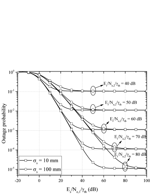
Figure 1: OP vs $\frac{E_{s}/N_{o,1}}{\gamma_{th}}$, for different values of $\frac{E_{r}/N_{o,2}}{\gamma_{th}}$ and $\sigma_{s}$.

Fig. 1 presents the outage performance of the mixed THz-RF wireless system as a function of $\frac{E_{s}/N_{o,1}}{\gamma_{th}}$, for different values of $\frac{E_{r}/N_{o,1}}{\gamma_{th}}$ and $\sigma_{s}$. As expected, for a given $\frac{E_{r}/N_{o,2}}{\gamma_{th}}$ and $\sigma_{s}$, as $\frac{E_{s}/N_{o,1}}{\gamma_{th}}$ increases, the OP decreases. Moreover, for a fixed $\frac{E_{s}/N_{o,1}}{\gamma_{th}}$ and $\sigma_{s}$, as $\frac{E_{r}/N_{o,2}}{\gamma_{th}}$, the outage performance improves. Interestingly, the outage performance are constrained by the worst link. Finally, from this figure, it is seen that, for a given $\frac{E_{s}/N_{o,1}}{\gamma_{th}}$ and $\frac{E_{r}/N_{o,2}}{\gamma_{th}}$, as $\sigma_{s}$ increases, the outage performance degrades. This indicates the importance of taking into consideration the impact of antenna misalignment in the performance assessment of the mixed THz-RF wireless system.

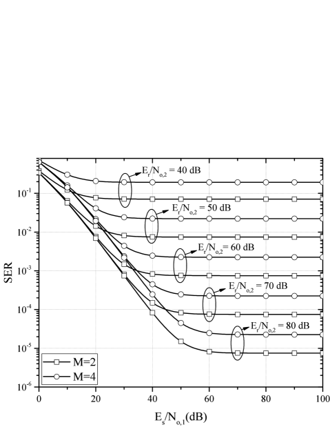
Figure 2: SER vs ${E_{s}/N_{o,1}}$, for different values of ${E_{r}/N_{o,2}}$ and $M$.

Fig. 2, the SER of a mixed THz-RF wireless system, which employs $M-$QAM, as a function of ${E_{s}/N_{o,1}}$, for different values of ${E_{r}/N_{o,2}}$ and $M$ is plotted. Note that $M=2$ corresponds to the SER performance of BPSK. We observe that, for a given ${E_{r}/N_{o,2}}$ and $M$, as ${E_{s}/N_{o,1}}$ increases, the error performance improves. Similarly, for a fixed ${E_{s}/N_{o,1}}$ and $M$, as ${E_{r}/N_{o,2}}$ increases, the SER decreases. Meanwhile, we observe that the minimum SER is determined by the transmission SNR of the worst link. Finally, for given ${E_{s}/N_{o,1}}$ and ${E_{r}/N_{o,2}}$, as $M$ increases, the error performance degrades. This indicates that in order to improve the error performance of the mixed THz-RF wireless system, we can either increase the transmission SNR of the worst link, or decrease $M$.

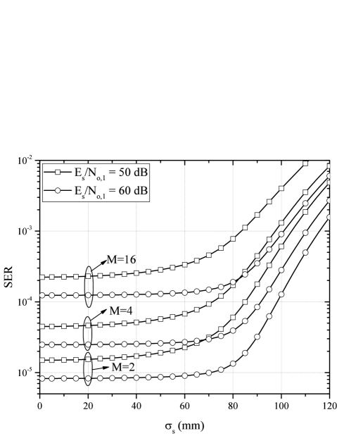
Figure 3: SER vs $\sigma_{s}$, for different values of ${E_{s}/N_{o,1}}$ and $M$.

Fig. 3, the SER of a mixed THz-RF wireless system, which employs $M-$QAM, as a function of $\sigma_{s}$, for different values of ${E_{s}/N_{o,1}}$ and $M$, assuming ${E_{r}/N_{o,2}}=80\text{ }\mathrm{dB}$, is depicted. From this figure, we observe that, for fixed ${E_{s}/N_{o,1}}$ and $M$, as $\sigma_{s}$ increases, the error performance degrades. Moreover, for given $\sigma_{s}$ and $M$, as ${E_{s}/N_{o,1}}$ increases, the error performance improves, whereas, for fixed $\sigma_{s}$ and ${E_{s}/N_{o,1}}$, as $M$ increases, the SER also increases. Finally, it is noticeable that in the relatively low $\sigma_{s}$ regime, the decrease of $M$ causes a more significantly boost in the error performance of the mixed THz-RF wireless system compared to the one that is caused by the increase of ${E_{s}/N_{o,1}}$. The reverse happens in the high $\sigma_{s}$ regime. This reveals the importance of taking into account the impact of antenna misalignment in the design of adaptive modulation and power allocation algorithms.

V Conclusions

This letter introduced the mixed THz-RF wireless system architecture and provided its outage and error performance assessment study. Specifically, novel closed-form expressions for the OP and SER were extracted, which accurately quantify the system performance and takes into consideration the transceivers characteristics and both the THz and RF channel particularities. Our results revealed that the performance of the mixed THz-RF wireless system are constrained from the quality of the worst link as well as the importance of taking into account the impact of the THz antenna misalignment, when assessing the system reliability.

Appendix

Appendix A

Based on (8), the CDF of $\gamma_{e}$ can be obtained as

$$F_{\gamma_{e}}\left(x\right)=F_{\gamma_{1}}\left(x\right)+F_{\gamma_{2}}\left(x\right)-F_{\gamma_{1}}\left(x\right)F_{\gamma_{2}}\left(x\right),$$ (14)

where $F_{\gamma_{1}}\left(\cdot\right)$ and $F_{\gamma_{2}}\left(\cdot\right)$ are respectively the CDFs of $\gamma_{1}$ and $\gamma_{2}$. Next, we provide closed form expressions for $F_{\gamma_{1}}\left(\cdot\right)$ and $F_{\gamma_{2}}\left(\cdot\right)$.

The CDF of $\gamma_{1}$ can be analytically evaluated as $F_{\gamma_{1}}\left(x\right)=P_{r}\left(\gamma_{1}\leq x\right),$ which, according to (9), can be rewritten as

$$F_{\gamma_{1}}\left(x\right)=F_{\left|h_{pf}\right|}\left(\sqrt{\frac{xN_{o,1}}{\left|h_{l}\right|^{2}E_{s}}}\right),$$ (15)

or equivalently

$$F_{\gamma_{1}}\left(x\right)=1-\frac{1}{\alpha}\left(\frac{N_{o,1}}{\left|h_{l}\right|^{2}E_{s}}\right)^{\phi/2}\frac{x^{\phi/2}}{\hat{h}_{f}^{\phi}}\frac{\phi}{S_{0}^{\phi}}$$

$$\times\sum_{k=0}^{\mu-1}\frac{\mu^{\frac{\phi}{\alpha}}}{k!}\Gamma\left(\frac{\alpha k-\phi}{\alpha},{\mu\left(\frac{N_{o,1}}{\left|h_{l}\right|^{2}E_{s}}\right)^{\alpha/2}\frac{x^{\alpha/2}}{\hat{h}_{f}^{\alpha}S_{0}^{\alpha}}}\right).$$ (16)

Similarly, since $|h_{f}|$ follows a Rayleigh distribution, $|h_{f}|^{2}$ follows an exponential distribution; hence, $\gamma_{2}$ also follows an exponential distribution with CDF that can be obtained as

$$F_{\gamma_{2}}\left(x\right)=1-\exp{\left(-\frac{N_{o,2}x}{|h_{g}|^{2}E_{r}}\right)}.$$ (17)

By substituting (16) and (17) into (14) and after some algebraic manipulations, we get (10). This concludes the proof.

Appendix B

By assuming two-dimensional modulation, the conditional SER can be obtained as [19]

$$P_{e}(x)=a\mathrm{Q}\left(\sqrt{2bx}\right).$$ (18)

Note that for several Gray bit-mapped constellations, the conditional SER can be expressed in this form [20, 21]. Thus, the average SER can be expressed as

$$\overline{P}_{e}=\int_{0}^{\infty}P_{e}\left(x\right)f_{\gamma_{e}}(x)\mathrm{dx},$$ (19)

or equivalently

$$\overline{P}_{e}=-\int_{0}^{\infty}F_{\gamma_{e}}(x)f_{e}(x)\mathrm{dx}$$ (20)

where $f_{{e}}(x)$ can be evaluated as $f_{e}(x)=\frac{\mathrm{d}P_{e}\left(x\right)}{\mathrm{dx}},$ or

$$f_{e}(x)=-a\sqrt{\frac{b}{4\pi}}x^{-1/2}\exp\left(-bx\right).$$ (21)

By substituting (10) and (21) into (20), we can write (20) as

$$\overline{P}_{e} =\mathcal{I}_{1}-a\sqrt{\frac{b}{4\pi}}\frac{\phi}{\alpha}\left(\frac{N_{o,1}}{S_{0}^{2}\hat{h}_{f}^{2}\left|h_{l}\right|^{2}E_{s}}\right)^{\phi/2}\sum_{k=0}^{\mu-1}\frac{\mu^{\frac{\phi}{\alpha}}}{k!}\mathcal{I}_{2}(k),$$ (22)

where

$$\mathcal{I}_{1}=a\sqrt{\frac{b}{4\pi}}\int_{0}^{\infty}x^{-1/2}\exp\left(-bx\right)\mathrm{dx}$$ (23)

and

$$\mathcal{I}_{2}(k) =\int_{0}^{\infty}x^{\left(\phi-1\right)/2}\exp{\left(-\left(\frac{N_{o,2}}{|h_{g}|^{2}E_{r}}+b\right)x\right)}$$

$$\times\Gamma\left(\frac{\alpha k-\phi}{\alpha},{\mu\left(\frac{N_{o,1}}{\left|h_{l}\right|^{2}E_{s}}\right)^{\alpha/2}\frac{x^{\alpha/2}}{\hat{h}_{f}^{\alpha}S_{0}^{\alpha}}}\right)\mathrm{dx}.$$ (24)

By employing [16, eq. (3.326/2)], (23) can be analytically evaluated as

$$\mathcal{I}_{1}=\frac{a}{2},$$ (25)

while by using [16, eq. (8.352/2)], (24) can be rewritten as

$$\mathcal{I}_{2}(k) =\int_{0}^{\infty}x^{\left(\phi-1\right)/2}\Gamma\left(1,\left(\frac{N_{o,2}}{|h_{g}|^{2}E_{r}}+b\right)x\right)$$

$$\times\Gamma\left(\frac{\alpha k-\phi}{\alpha},{\mu\left(\frac{N_{o,1}}{\left|h_{l}\right|^{2}E_{s}}\right)^{\alpha/2}\frac{x^{\alpha/2}}{\hat{h}_{f}^{\alpha}S_{0}^{\alpha}}}\right)\mathrm{dx}.$$ (26)

Moreover, by employing [22, eq. (5)], (26) can be obtained as

$$\mathcal{I}_{2}(k)=\int_{0}^{\infty}x^{\left(\phi-1\right)/2}G_{1,2}^{2,0}\left(\left(\frac{N_{o,2}}{|h_{g}|^{2}E_{r}}+b\right)x\left|\begin{array}[]{c}1\\ 1,0\end{array}\right.\right)$$ (29)

$$\times G_{1,2}^{2,0}\left(\left(\frac{N_{o,1}}{\left|h_{l}\right|^{2}E_{s}}\right)^{\alpha/2}\frac{\mu}{\hat{h}_{f}^{\alpha}S_{0}^{\alpha}}x^{\alpha/2}\left|\begin{array}[]{c}1\\ \frac{\alpha k-\phi}{\alpha},0\end{array}\right.\right)\mathrm{dx},$$ (32)

which, based on [23, Ch. 2.3], can be written in closed-form as

$$\mathcal{I}_{2}(k)=\left(\frac{N_{o,2}}{|h_{g}|^{2}E_{r}}+b\right)^{-\frac{\phi+1}{2}}$$

$$\times H_{3,3}^{2,2}\left(\frac{\mu\left(\frac{N_{o,1}}{\left|h_{l}\right|^{2}E_{s}}\right)^{\alpha/2}\frac{1}{\hat{h}_{f}^{\alpha}S_{0}^{\alpha}}}{\left(\frac{N_{o,2}}{|h_{g}|^{2}E_{r}}+b\right)^{\alpha/2}}\left|\begin{array}[]{c}\left(-\frac{\phi+1}{2},\frac{\alpha}{2}\right),\left(\frac{1-\phi}{2},\frac{\alpha}{2}\right),\left(1,1\right)\\ \left(\frac{\alpha k-\phi}{\alpha},1\right),\left(0,1\right),\left(-\frac{\phi+1}{2},\frac{\alpha}{2}\right)\end{array}\right.\right).$$ (35)

Finally, by substituting (23) and (35) into (22), we obtain (13). This concludes the proof.

References

- [1] A.-A. A. Boulogeorgos, A. Alexiou, T. Merkle, C. Schubert, R. Elschner, A. Katsiotis, P. Stavrianos, D. Kritharidis, P. K. Chartsias, J. Kokkoniemi, M. Juntti, J. Lehtomäki, A. Teixeirá, and F. Rodrigues, “Terahertz technologies to deliver optical network quality of experience in wireless systems beyond 5G,” IEEE Commun. Mag., vol. 56, no. 6, pp. 144–151, Jun. 2018.
- [2] A.-A. A. Boulogeorgos, A. Alexiou, D. Kritharidis, A. Katsiotis, G. Ntouni, J. Kokkoniemi, J. Lethtomaki, M. Juntti, D. Yankova, A. Mokhtar, J.-C. Point, J. Machodo, R. Elschner, C. Schubert, T. Merkle, R. Ferreira, F. Rodrigues, and J. Lima, “Wireless terahertz system architectures for networks beyond 5G,” TERRANOVA CONSORTIUM, White paper 1.0, Jul. 2018.
- [3] A.-A. A. Boulogeorgos, S. Goudos, and A. Alexiou, “Users association in ultra dense THz networks,” in IEEE International Workshop on Signal Processing Advances in Wireless Communications (SPAWC), Kalamata, Greece, Jun. 2018.
- [4] J. M. Jornet and I. F. Akyildiz, “Channel modeling and capacity analysis for electromagnetic wireless nanonetworks in the terahertz band,” IEEE Trans. Wireless Commun., vol. 10, no. 10, pp. 3211–3221, Oct. 2011.
- [5] J. Kokkoniemi, J. Lehtomäki, and M. Juntti, “Simplified molecular absorption loss model for 275-400 gigahertz frequency band,” in 12th European Conference on Antennas and Propagation (EuCAP), London, UK, Apr. 2018.
- [6] A.-A. A. Boulogeorgos, E. N. Papasotiriou, J. Kokkoniemi, J. Lehtomäki, A. Alexiou, and M. Juntti, “Performance evaluation of THz wireless systems operating in 275-400 GHz band,” IEEE Vehicular Technology Conference (VTC), 2018.
- [7] J. Kokkoniemi, J. Lehtomäki, and M. Juntti, “Frequency domain scattering loss in THz band,” in Global Symposium on Millimeter-Waves (GSMM), Montreal, Canada, May 2015, pp. 1–3.
- [8] A. R. Ekti, A. Boyaci, A. Alparslan, . Ünal, S. Yarkan, A. Görçin, H. Arslan, and M. Uysal, “Statistical modeling of propagation channels for terahertz band,” in IEEE Conference on Standards for Communications and Networking (CSCN), Helsinki, Finland, Sep. 2017, pp. 275–280.
- [9] S. Priebe, C. Jastrow, M. Jacob, T. Kleine-Ostmann, T. Schrader, and T. Kurner, “Channel and propagation measurements at 300 GHz,” IEEE Trans. Antennas Propag., vol. 59, no. 5, pp. 1688–1698, May 2011.
- [10] C. Han and I. F. Akyildiz, “Three-dimensional end-to-end modeling and analysis for graphene-enabled terahertz band communications,” IEEE Trans. Veh. Technol., vol. 66, no. 7, pp. 5626–5634, Jul. 2017.
- [11] A.-A. A. Boulogeorgos, E. N. Papasotiriou, and A. Alexiou, “Analytical performance assessment of THz wireless systems,” IEEE Access, vol. 7, no. 1, pp. 1–18, Jan. 2019.
- [12] M. K. Simon and M. S. Alouini, Digital Communication over Fading Channels, 2nd ed. Newark, NJ: Wiley, 2005. [Online]. Available: https://cds.cern.ch/record/994549
- [13] T. T. Duy, T. Duong, D. Benevides da Costa, V. N. Q. Bao, and M. Elkashlan, “Proactive relay selection with joint impact of hardware impairment and co-channel interference,” IEEE Trans. Commun., vol. 63, no. 5, pp. 1594–1606, May 2015.
- [14] E. Björnson, M. Matthaiou, and M. Debbah, “A new look at dual-hop relaying: Performance limits with hardware impairments,” IEEE Trans. Commun., vol. 61, no. 11, pp. 4512–4525, Nov. 2013.
- [15] A. E. Canbilen, S. S. Ikki, E. Basar, S. S. Gultekin, and I. Develi, “Impact of I/Q imbalance on amplify-and-forward relaying: Optimal detector design and error performance,” IEEE Trans. Commun., vol. 67, no. 5, pp. 3154–3166, May 2019.
- [16] I. S. Gradshteyn and I. M. Ryzhik, Table of Integrals, Series, and Products, 6th ed. New York: Academic, 2000.
- [17] N. V. Savoschenko, Special Integral Functions Used in Wireless Communications Theory. Singapore: World Scientific Publishing Co. Pte. Ltd., 2014.
- [18] A. P. Prudnikov, Y. A. Brychkov, and O. I. Marichev, Integral and Series: Volume 3, More Special Functions. CRC Press Inc., 1990.
- [19] J. Proakis, Digital Communications, 4th ed. NY: McGraw-Hill, 2001.
- [20] O. Amin, S. S. Ikki, and M. Uysal, “On the performance analysis of multirelay cooperative diversity systems with channel estimation errors,” IEEE Trans. Veh. Technol., vol. 60, no. 5, pp. 2050–2059, Jun. 2011.
- [21] S. S. Ikki and M. H. Ahmed, “Performance analysis of adaptive decode-and-forward cooperative diversity networks with best-relay selection,” IEEE Trans. Commun., vol. 58, no. 1, pp. 68–72, Jan. 2010.
- [22] S. Kumar, “Exact evaluations of some Meijer G-functions and probability of all eigenvalues real for the product of two gaussian matrices,” J. Phys. A: Math. Theor., vol. 48, no. 44, p. 445206, Oct. 2015.
- [23] A. M. Mathai, R. K. Saxena, and H. J. Haubold, The H-Function: Theory and Applications. New York Dordrecht Heidelberg London: Springer, 2010.