Inverse LDM^T and LU Factorizations of a Partitioned Matrix with the Square-root and Division Free Version for V-BLAST

Abstract

This letter proposes the inverse LDM^T and LU factorizations of a matrix partitioned into $2\times 2$ blocks, which include the square-root and division free version. The proposed square-root and division free inverse LDM^T factorization is applied to compute the initial estimation error covariance matrix $\mathbf{Q}$ for the recursive V-BLAST algorithm, which can save $K-1$ divisions (where $K$ is the number of transmit antennas), and requires about the same computational complexity as the corresponding algorithm to compute $\mathbf{Q}$ in the existing recursive V-BLAST algorithm [8, 9]. The proposed square-root and division free inverse LDM^T factorization can also be applied to propose the square-root and division free implementation for the square-root V-BLAST algorithm in [5], where the wide-sense Givens rotation in [14] is utilized. With respect to the existing square-root V-BLAST algorithms [5, 6], the proposed square-root and division free V-BLAST algorithm requires about the same computational complexity, and can avoid the square-root and division operations.

I Introduction

Multiple-input multiple output (MIMO) wireless communication systems can achieve very high spectral efficiency in rich multi-path environments [1]. Bell Labs Layered Space-Time architecture (BLAST), including the relative simple vertical BLAST (V-BLAST), is such a system that transmits independent data streams simultaneously from multiple antennas [2] to maximize the data rate. V-BLAST usually utilizes the ordered successive interference cancellation (OSIC) detector [2], to detect the data streams iteratively with the optimal ordering. In each iteration, the OSIC detector utilizes a zero-forcing (ZF) or minimum mean-square error (MMSE) filter to detect the data stream with the highest signal-to-noise ratio (SNR) among all undetected data streams, and then subtracts the effect of the detected data stream in the received signal vector.

The OSIC detector for V-BLAST requires high computational complexity. Thus fast algorithms have been proposed for V-BLAST [3]-[9], of which typical examples are the square-root algorithms [3]-[6] and the recursive algorithms [7]-[9]. In the OSIC detection phase, the recursive V-BLAST algorithms update the estimation error covariance matrix $\mathbf{Q}={\mathbf{R}}^{-1}$ recursively, while the square-root V-BLAST algorithms update the square-root of $\mathbf{Q}$, i.e., ${\bf{\Gamma}}$ satisfying ${\bf{\Gamma}}{\bf{\Gamma}}^{H}={\bf{Q}}$.

In fixed-point implementations, it is highly desirable to avoid square-root and division operations, since they are demanding in terms of the required bit precision and clock cycles [10, 11]. To compute the initial square-root ${\bf{\Gamma}}$, the inverse Cholesky factorization in [5] and the corresponding algorithm in [6] (by the Cholesky factorization and the back-substitution [12]) both reduce half divisions. Moreover, to implement a spherical MIMO detector, the alternative Cholesky factorization was proposed in [10] to avoid both square-root and division operations. This letter makes progress along this direction, and gives an efficient square-root and division free algorithm to compute the initial square-root for the square-root V-BLAST algorithm, which can also be utilized to compute the initial $\mathbf{Q}$ for the recursive V-BLAST algorithm.

In Matlab, the “inv” function [13] for the matrix inversion computes the $\mathbf{LU}$ factors of a matrix $\mathbf{R}$, inverts the $\mathbf{LU}$ factors, and multiplies the inverses to obtain $\mathbf{Q}=\mathbf{R}^{-1}$. When $\mathbf{R}$ is Hermitian, the $\mathbf{LU}$ factors become the ${\mathbf{LDL}}^{T}$ factors [13]. This letter proposes the improved implementations for the inversion algorithm in the Matlab “inv” function, which can be utilized in V-BLAST. We propose an efficient inverse ${\mathbf{LDM}}^{T}$ factorization to compute the $(k+i)^{th}$ order inverse ${\mathbf{LDM}}^{T}$ factors from the $k^{th}$ order inverse ${\mathbf{LDM}}^{T}$ factors by just one iteration, where $k$ and $i$ can be any positive integers. Then the proposed inverse ${\mathbf{LDM}}^{T}$ factorization is transformed into the proposed inverse ${\mathbf{LU}}^{T}$ factorization. Moreover, from the proposed inverse ${\mathbf{LDM}}^{T}$ factorization, we deduce the alternative division-free inverse ${\mathbf{LDM}}^{T}$ factorization, which is utilized by the recursive V-BLAST algorithm [8, 9] to compute the initial ${\mathbf{Q}}$, and is also applied to develop a full square-root and division free implementation of the square-root V-BLAST algorithm in [5].

The V-BLAST System model is overviewed in Section ii@. Section iii@ proposes the inverse LDM^T and LU factorizations with the square-root and division free version. Then the proposed square-root and division free inverse LDM^T factorization is applied in V-BLAST in Section iv@. The complexity of the presented algorithms is evaluated in Section v@. Finally, we make conclusion in Section vi@.

II V-BLAST System Model

The considered V-BLAST system consists of $K$ transmit antennas and $N(\geq K)$ receive antennas in a rich-scattering and flat-fading wireless channel. At the transmitter, the data stream is de-multiplexed into $K$ sub-streams. Then each sub-stream is encoded and fed to its respective transmit antenna. Let ${\bf{s}}=[s_{1},s_{2},\cdots,s_{K}]^{T}$ denote the vector of transmit symbols from $K$ antennas, and assume $E({\bf{ss}}^{H})=\sigma_{{s}}^{2}{\bf{{\rm I}}}_{K}$ where ${\bf{{I}}}_{K}$ is the identity matrix with size $K$. Then the received symbol vector is

$${\bf{x}}={\bf{H}}\cdot{\bf{s}}+{\bf{n}},$$ (1)

where ${\bf{n}}$ is the $N\times 1$ complex Gaussian noise vector with zero mean and covariance $\sigma_{n}^{2}{\bf{{\rm I}}}_{N}$, and ${\bf{H}}$ is the $N\times K$ complex channel matrix with statistically independent entries.

The minimum mean-square error (MMSE) detection of $\bf{s}$ is

$${\bf{\hat{s}}}=\left({{\bf{H}}^{H}{\bf{H}}+\alpha{\bf{I}}_{K}}\right)^{-1}{\bf{H}}^{H}{\bf{x}},$$ (2)

where $\alpha=\sigma_{n}^{2}/\sigma_{s}^{2}$, $(\bullet)^{-1}$ and $(\bullet)^{H}$ denote matrix inversion and matrix conjugate transposition, respectively. Let

$${\bf{R}}={\bf{H}}^{H}\cdot{\bf{H}}+\alpha{\bf{I}}_{K}.$$ (3)

The estimation error covariance matrix is [3]

$${\bf{Q}}={\bf{R}}^{-1}=\left({{\bf{H}}^{H}{\bf{H}}+\alpha{\bf{I}}_{K}}\right)^{-1},$$ (4)

and the square-root of ${\bf{Q}}$ is ${\bf{\Gamma}}$ satisfying

$${\bf{\Gamma}}{\bf{\Gamma}}^{H}={\bf{Q}}.$$ (5)

The conventional V-BLAST detects $K$ entries of ${\bf{s}}$ by $K$ iterations with the optimal ordering. In the $k^{th}$ ($k=K,K-1,\cdots,2$) iteration, the entry with the highest post detection signal-to-noise ratio (SNR) among all the undetected $k$ entries is detected by a linear MMSE or zero-forcing (ZF) filter. Then its effect is subtracted from the received symbol vector [2, 3], and accordingly ${\bf{Q}}_{|(k-1)}$ or ${\bf{\Gamma}}_{|(k-1)}$ corresponding to all the undetected $k-1$ entries needs to be computed.

The first $k$ columns of ${\bf{H}}$ can be represented as

$${\bf{H}}_{k}=[{\bf{h}}_{1},{\bf{h}}_{2},...,{\bf{h}}_{k}],$$ (6)

where ${\bf{h}}_{m}$ ($1\leq m\leq k$) denotes the $m^{th}$ column of ${\bf{H}}$. Then ${\bf{R}}_{k}$ and ${\bf{Q}}_{k}$ are defined from ${\bf{H}}_{k}$ by (3) and (4), respectively, while ${\bf{R}}_{k+1}$ satisfies [7]

$${\bf{R}}_{k+1}=\\ \left[{\begin{array}[]{*{20}c}{{\bf{R}}_{k}}&{\bf{H}}_{k}^{H}{\bf{h}}_{k+1}\\ {\bf{h}}_{k+1}^{H}{\bf{H}}_{k}&{\bf{h}}_{k+1}^{H}{\bf{h}}_{k+1}+\alpha\\ \end{array}}\right]=\left[{\begin{array}[]{*{20}c}{{\bf{R}}_{k}}&{{\bf{v}}}\\ {{\bf{v}}^{H}}&t\\ \end{array}}\right].$$ (7)

III Efficient Inverse LDM^T and LU Factorizations of a Partitioned Matrix

Assume that $i$ rows and columns are added to a $k\times k$ general square matrix ${{\mathbf{R}}_{k}}$ to form a $(k+i)\times(k+i)$ matrix ${{\mathbf{R}}_{k+i}}$, which is written as a matrix partitioned into $2\times 2$ blocks, i.e.,

$$\mathbf{R}_{k+i}=\left[\begin{matrix}{{\mathbf{R}}_{k}}&\mathbf{V}\\ {{\mathbf{Y}}^{H}}&\mathbf{T}\\ \end{matrix}\right].$$ (8)

Obviously (7) is a special case of (8) with $i=1$ and the Hermitian $\mathbf{R}_{k+i}$. The upper-triangular LDM^T factors of ${{\mathbf{R}}}^{-1}={{\mathbf{Q}}}$ satisfy

$$\mathbf{LD}{{\mathbf{M}}^{H}}={{\mathbf{R}}^{-1}}={{\mathbf{Q}}},$$ (9)

from which we can deduce

$${{\mathbf{M}}^{-H}}{{\mathbf{D}}^{-1}}{{\mathbf{L}}^{-1}}=\mathbf{R},$$ (10)

where ${{\mathbf{M}}^{-H}}$ and ${{\mathbf{L}}^{-H}}$ are the conventional lower-triangular LDM^T factors [12] of ${{\mathbf{R}}}$.

III-A Inverse LDM^T Factorization of a Partitioned Matrix

Obviously the upper-triangular LDM^T factors of ${{\mathbf{R}}_{k+i}^{-1}}$ satisfy

$${{\mathbf{L}}_{k+i}}\text{=}\left[\begin{matrix}{{\mathbf{L}}_{k}}&\mathbf{A}\\ \mathbf{0}&\mathbf{F}\\ \end{matrix}\right]$$ (11a)

$${{\mathbf{D}}_{k+i}}=\left[\begin{matrix}{{\mathbf{D}}_{k}}&\mathbf{0}\\ \mathbf{0}&\mathbf{G}\\ \end{matrix}\right]$$ (11b)

$${{\mathbf{M}}_{k+i}}\text{=}\left[\begin{matrix}{{\mathbf{M}}_{k}}&\mathbf{B}\\ \mathbf{0}&\mathbf{E}\\ \end{matrix}\right].$$ (11c)

In (11c), $\mathbf{A}$, $\mathbf{F}$, $\mathbf{G}$, $\mathbf{B}$ and $\mathbf{E}$ can be computed by

$$\mathbf{A}=-\mathbf{L}_{k}\mathbf{D}_{k}\mathbf{M}_{k}^{H}\mathbf{VF}$$ (12a)

$${{\mathbf{B}}^{H}}=-{{\mathbf{E}}^{H}}{{\mathbf{Y}}^{H}}\mathbf{L}_{k}\mathbf{D}_{k}\mathbf{M}_{k}^{H}$$ (12b)

$$\mathbf{FG}{{\mathbf{E}}^{H}}={{(\mathbf{T}-{{\mathbf{Y}}^{H}}\mathbf{L}_{k}\mathbf{D}_{k}\mathbf{M}_{k}^{H}\mathbf{V})}^{-1}},$$ (12c)

where the diagonal $\mathbf{G}$, the upper-triangular $\mathbf{F}$ and ${{\mathbf{E}}}$ are the inverse $\mathbf{LD}\mathbf{M}^{H}$ factors of $\mathbf{T}-{{\mathbf{Y}}^{H}}\mathbf{L}_{k}\mathbf{D}_{k}\mathbf{M}_{k}^{H}\mathbf{V}$ in (12c). The derivation of (12c) is as follows.

From (11c) we can deduce $\mathbf{L}_{k+i}^{-1}\text{=}\left[\begin{matrix}\mathbf{L}_{k}^{-1}&\text{-}\mathbf{L}_{k}^{-1}\mathbf{A}{{\mathbf{F}}^{-1}}\\ \mathbf{0}&{{\mathbf{F}}^{-1}}\\ \end{matrix}\right]$, $\mathbf{D}_{k+i}^{-1}=\left[\begin{matrix}\mathbf{D}_{k}^{-1}&\mathbf{0}\\ \mathbf{0}&{{\mathbf{G}}^{-1}}\\ \end{matrix}\right]$ and $\mathbf{M}_{k+i}^{-1}\text{=}\left[\begin{matrix}\mathbf{M}_{k}^{-1}&\text{-}\mathbf{M}_{k}^{-1}\mathbf{B}{{\mathbf{E}}^{-1}}\\ \mathbf{0}&{{\mathbf{E}}^{-1}}\\ \end{matrix}\right]$, which are substituted into (10) to obtain

$$\left[\begin{matrix}\mathbf{M}_{k}^{-H}&\mathbf{0}\\ -{{\mathbf{E}}^{-H}}{{\mathbf{B}}^{H}}\mathbf{M}_{k}^{-H}&{{\mathbf{E}}^{-H}}\\ \end{matrix}\right]\left[\begin{matrix}\mathbf{D}_{k}^{-1}&\mathbf{0}\\ \mathbf{0}&{{\mathbf{G}}^{-1}}\\ \end{matrix}\right]\\ \times\left[\begin{matrix}\mathbf{L}_{k}^{-1}&-\mathbf{L}_{k}^{-1}\mathbf{A}{{\mathbf{F}}^{-1}}\\ \mathbf{0}&{{\mathbf{F}}^{-1}}\\ \end{matrix}\right]=\mathbf{R}_{k+i}.$$ (13)

We can substitute (8) into (13) to deduce

$$\left[{\begin{array}[]{*{20}{c}}{{\bf{M}}_{k}^{-H}{\bf{D}}_{k}^{-1}{\bf{L}}_{k}^{-1}}&{-{\bf{M}}_{k}^{-H}{\bf{D}}_{k}^{-1}{\bf{L}}_{k}^{-1}{\bf{A}}{{\bf{F}}^{-1}}}\\ {\left(\begin{array}[]{l}{\rm{-}}{{\bf{E}}^{-H}}\times\\ {{\bf{B}}^{H}}{\bf{M}}_{k}^{-H}\times\\ {\bf{D}}_{k}^{-1}{\bf{L}}_{k}^{-1}\end{array}\right)}&{\left(\begin{array}[]{l}{{\bf{E}}^{-H}}{{\bf{B}}^{H}}{\bf{M}}_{k}^{-H}\times\\ {\bf{D}}_{k}^{-1}{\bf{L}}_{k}^{-1}{\bf{A}}{{\bf{F}}^{-1}}+\\ {{\bf{E}}^{-H}}{{\bf{G}}^{-1}}{{\bf{F}}^{-1}}\end{array}\right)}\end{array}}\right]\\ =\left[{\begin{array}[]{*{20}{c}}{{{\bf{R}}_{k}}}&{\bf{V}}\\ {{{\bf{Y}}^{H}}}&{\bf{T}}\end{array}}\right],$$ (14)

from which we can obtain

$$-\mathbf{M}_{k}^{{\text{-}}H}\mathbf{D}_{k}^{{\text{-}}1}\mathbf{L}_{k}^{{\text{-}}1}\mathbf{A}{{\mathbf{F}}^{{\text{-}}1}}=\mathbf{V}$$ (15a)

$$-{{\mathbf{E}}^{{\text{-}}H}}{{\mathbf{B}}^{H}}\mathbf{M}_{k}^{{\text{-}}H}\mathbf{D}_{k}^{{\text{-}}1}\mathbf{L}_{k}^{{\text{-}}1}={{\mathbf{Y}}^{H}}$$ (15b)

$${{\mathbf{E}}^{{\text{-}}H}}{{\mathbf{B}}^{H}}\mathbf{M}_{k}^{{\text{-}}H}\mathbf{D}_{k}^{{\text{-}}1}\mathbf{L}_{k}^{{\text{-}}1}\mathbf{A}{{\mathbf{F}}^{{\text{-}}1}}+{{\mathbf{E}}^{{\text{-}}H}}{{\mathbf{G}}^{{\text{-}}1}}{{\mathbf{F}}^{{\text{-}}1}}=\mathbf{T}.$$ (15c)

From (15a) and (15b) , we can deduce (12a) and (12b) , respectively. Then we substitute (12a) and (12b) into (15c) to obtain ${{\mathbf{Y}}^{H}}\mathbf{L}_{k}\mathbf{D}_{k}\mathbf{M}_{k}^{H}\mathbf{V}+{{\mathbf{E}}^{-H}}{{\mathbf{G}}^{-1}}{{\mathbf{F}}^{-1}}=\mathbf{T}$, from which we can deduce (12c) .

III-B Inverse LU Factorization of a Partitioned Matrix

Substitute (12c) into (11c), and substitute (11c) into (9) to obtain

$$\left[\begin{matrix}{{\mathbf{L}}_{k}}&-\mathbf{L}_{k}\mathbf{D}_{k}\mathbf{M}_{k}^{H}\mathbf{VF}\\ \mathbf{0}&\mathbf{F}\\ \end{matrix}\right]\left[\begin{matrix}{{\mathbf{D}}_{k}}&\mathbf{0}\\ \mathbf{0}&\mathbf{G}\\ \end{matrix}\right]\times\\ \left[\begin{matrix}{{\mathbf{M}}_{k}^{H}}&\mathbf{0}\\ -{{\mathbf{E}}^{H}}{{\mathbf{Y}}^{H}}\mathbf{L}_{k}\mathbf{D}_{k}\mathbf{M}_{k}^{H}&\mathbf{E}^{H}\\ \end{matrix}\right]=\mathbf{R}_{k+i}^{-1}.$$ (16)

From (16) we can deduce

$$\left[\begin{matrix}{{\mathbf{L}}_{k}}&-{{\mathbf{L}}_{k}}{{\mathbf{D}}_{k}}{{\mathbf{M}}_{k}^{H}}\mathbf{VF}\\ \mathbf{0}&\mathbf{F}\\ \end{matrix}\right]\left[\begin{matrix}{{\mathbf{D}}_{k}}{{\mathbf{M}}_{k}^{H}}&\mathbf{0}\\ -\mathbf{G}{{\mathbf{E}}^{H}}{{\mathbf{Y}}^{H}}{{\mathbf{L}}_{k}}{{\mathbf{D}}_{k}}{{\mathbf{M}}_{k}^{H}}&\mathbf{G}{{\mathbf{E}}^{H}}\\ \end{matrix}\right]\\ =\mathbf{R}_{k+i}^{-1}.$$ (17)

Let ${{\mathbf{U}}_{k}}={{\mathbf{D}}_{k}}\mathbf{M}_{k}^{H}$, $\mathbf{P}=\mathbf{G}{{\mathbf{E}}^{H}}$, which can be substituted into (17) and (12c) to obtain

$$\left[\begin{matrix}{{\mathbf{L}}_{k}}&-{{\mathbf{L}}_{k}}{{\mathbf{U}}_{k}}\mathbf{VF}\\ \mathbf{0}&\mathbf{F}\\ \end{matrix}\right]\left[\begin{matrix}{{\mathbf{U}}_{k}}&\mathbf{0}\\ -\mathbf{P}{{\mathbf{Y}}^{H}}{{\mathbf{L}}_{k}}{{\mathbf{U}}_{k}}&\mathbf{P}\\ \end{matrix}\right]=\mathbf{R}_{k+i}^{-1}$$ (18)

and

$$\mathbf{FP}={{(\mathbf{T}-{{\mathbf{Y}}^{H}}{{\mathbf{L}}_{k}}{{\mathbf{U}}_{k}}\mathbf{V})}^{-1}},$$ (19)

respectively. From (18) we can deduce

$${{{{\mathbf{L}}_{k+i}}}}=\left[\begin{matrix}{{\mathbf{L}}_{k}}&-{{\mathbf{L}}_{k}}{{\mathbf{U}}_{k}}\mathbf{VF}\\ \mathbf{0}&\mathbf{F}\\ \end{matrix}\right]$$ (20a)

$${{\mathbf{U}}_{k+i}}=\left[\begin{matrix}{{\mathbf{U}}_{k}}&\mathbf{0}\\ -\mathbf{P}{{\mathbf{Y}}^{H}}{{\mathbf{L}}_{k}}{{\mathbf{U}}_{k}}&\mathbf{P}\\ \end{matrix}\right],$$ (20b)

where $\mathbf{F}$ and $\mathbf{P}$ are the inverse LU factors satisfying (19).

III-C Division Free Inverse LDM^T Factorization

Let us try to use the alternative LDM^T factors of ${{\mathbf{R}}_{k}^{-1}}={\mathbf{Q}}_{k}$, which are assumed to be

$${\mathbf{\tilde{L}}}_{k}({\mathbf{\tilde{D}}}_{k}/{\delta}_{k}){{\mathbf{\tilde{M}}}_{k}^{H}}={\mathbf{L}}_{k}{\mathbf{D}}_{k}{{\mathbf{M}}_{k}^{H}}={{\mathbf{R}}_{k}^{-1}}={{\mathbf{Q}}_{k}}.$$ (21)

Substitute (21) into (12c) to obtain $\mathbf{FG}{{\mathbf{E}}^{H}}={{\left(\mathbf{T}-{{\mathbf{Y}}^{H}}{\mathbf{\tilde{L}}}_{k}({\mathbf{\tilde{D}}}_{k}/{\delta}_{k}){{\mathbf{\tilde{M}}}_{k}^{H}}\mathbf{V}\right)}^{-1}}$, i.e.,

$$\mathbf{F}(\mathbf{G}/{\delta}_{k}){{\mathbf{E}}^{H}}={{\left({\delta}_{k}\mathbf{T}-{{\mathbf{Y}}^{H}}{\mathbf{\tilde{L}}_{k}}{\mathbf{\tilde{D}}_{k}}{{\mathbf{\tilde{M}}}_{k}^{H}}\mathbf{V}\right)}^{-1}}.$$ (22)

Assume that the division free LDM^T factorization (21) is also utilized to obtain

$$\mathbf{\tilde{F}}(\mathbf{\tilde{G}}/\eta){{\mathbf{\tilde{E}}}^{H}}={{\left({\delta}_{k}\mathbf{T}-{{\mathbf{Y}}^{H}}{\mathbf{\tilde{L}}_{k}}{\mathbf{\tilde{D}}_{k}}{{\mathbf{\tilde{M}}}_{k}^{H}}\mathbf{V}\right)}^{-1}}.$$ (23)

By comparing (23) and (22) , we can deduce

$$\mathbf{\tilde{F}}({\delta}_{k}\mathbf{\tilde{G}}/\eta){{\mathbf{\tilde{E}}}^{H}}=\mathbf{FG}{{\mathbf{E}}^{H}}.$$ (24)

From (21) and (24) , we can write $\frac{{\mathbf{\tilde{D}}}_{k}}{{\delta}_{k}}={\mathbf{D}}_{k}$, ${\mathbf{\tilde{L}}}_{k}={\mathbf{L}}_{k}$, ${{\mathbf{\tilde{M}}}_{k}}={{{\mathbf{M}}_{k}}}$, $\frac{{\delta}_{k}}{\eta}\mathbf{\tilde{G}}=\mathbf{G}$, $\mathbf{\tilde{F}}=\mathbf{F}$ and ${{\mathbf{\tilde{E}}}^{H}}={{\mathbf{E}}^{H}}$, which are substituted into (16) to obtain

$$\left[\begin{matrix}{{\mathbf{\tilde{L}}}_{k}}&-{\mathbf{\tilde{L}}}_{k}\frac{{\mathbf{\tilde{D}}}_{k}}{{\delta}_{k}}{{\mathbf{\tilde{M}}}_{k}^{H}}\mathbf{V\tilde{F}}\\ \mathbf{0}&{\mathbf{\tilde{F}}}\\ \end{matrix}\right]\left[\begin{matrix}\frac{{\mathbf{\tilde{D}}}_{k}}{{\delta}_{k}}&\mathbf{0}\\ \mathbf{0}&\frac{{\delta}_{k}}{\eta}\mathbf{\tilde{G}}\\ \end{matrix}\right]\times\\ \left[\begin{matrix}{{\mathbf{\tilde{M}}}_{k}^{H}}&\mathbf{0}\\ -{{{\mathbf{\tilde{E}}}}^{H}}{{\mathbf{Y}}^{H}}{\mathbf{\tilde{L}}}_{k}\frac{{\mathbf{\tilde{D}}}_{k}}{{\delta}_{k}}{{\mathbf{\tilde{M}}}_{k}^{H}}&{{{\mathbf{\tilde{E}}}}^{H}}\\ \end{matrix}\right]=\mathbf{R}_{k+i}^{-1}.$$ (25)

To verify (25), we only need to substitute (21) and (24) into the left side of (25) (with the matrix multiplications finished), to verify that it is equal to the left side of (16) (with the matrix multiplications finished).

From (25) we can deduce

$$\left[\begin{matrix}{{\mathbf{\tilde{L}}}_{k}}&-{\mathbf{\tilde{L}}_{k}}{\mathbf{\tilde{D}}_{k}}{{\mathbf{\tilde{M}}}_{k}^{H}}\mathbf{V\tilde{F}}\\ \mathbf{0}&{\delta}_{k}\mathbf{\tilde{F}}\\ \end{matrix}\right]\left[\begin{matrix}\frac{{\mathbf{\tilde{D}}}_{k}}{{\delta}_{k}}&\mathbf{0}\\ \mathbf{0}&\frac{\mathbf{\tilde{G}}}{{\delta}_{k}\eta}\\ \end{matrix}\right]\times\\ \left[\begin{matrix}{{\mathbf{\tilde{M}}}_{k}^{H}}&\mathbf{0}\\ -{{\mathbf{Y}}^{H}}{\mathbf{\tilde{L}}_{k}}{\mathbf{\tilde{D}}_{k}}{{\mathbf{\tilde{M}}}_{k}^{H}}&{\delta}_{k}{{{\mathbf{\tilde{E}}}}^{H}}\\ \end{matrix}\right]=\mathbf{R}_{k+i}^{-1}.$$ (26)

Finally from (26), we can obtain

$${{\mathbf{\tilde{L}}}_{k+i}}=\left[\begin{matrix}{{{\mathbf{\tilde{L}}}}_{k}}&-{{{\mathbf{\tilde{L}}}}_{k}}{{{\mathbf{\tilde{D}}}}_{k}}\mathbf{\tilde{M}}_{k}^{H}\mathbf{V\tilde{F}}\\ \mathbf{0}&{\delta}_{k}\mathbf{\tilde{F}}\\ \end{matrix}\right]$$ (27a)

$$\mathbf{\tilde{M}}_{k+i}^{H}=\left[\begin{matrix}\mathbf{\tilde{M}}_{k}^{H}&\mathbf{0}\\ -{{\mathbf{Y}}^{H}}{{{\mathbf{\tilde{L}}}}_{k}}{{{\mathbf{\tilde{D}}}}_{k}}\mathbf{\tilde{M}}_{k}^{H}&{\delta}_{k}{{{\mathbf{\tilde{E}}}}^{H}}\\ \end{matrix}\right]$$ (27b)

$${{\mathbf{\tilde{D}}}_{k+i}}=\left[\begin{matrix}\eta{{{\mathbf{\tilde{D}}}}_{k}}&\mathbf{0}\\ \mathbf{0}&{\mathbf{\tilde{G}}}\\ \end{matrix}\right]$$ (27c)

$${{\delta}_{k+i}}={{\delta}_{k}}\eta,$$ (27d)

where $\mathbf{\tilde{F}}$, $\mathbf{\tilde{G}}$, ${{\mathbf{\tilde{E}}}}$ and $\eta$ are the division free LDM^T factors computed by (23).

IV Square-root and Division Free Inverse LDL^T Factorization for V-BLAST

When $i=1$, $\mathbf{V}$, ${{\mathbf{Y}}}$ and ${{\mathbf{T}}}$ in (8) and (27d) can be written as ${{\mathbf{v}}}$, $\mathbf{y}$ and $t$, respectively. We can use (23) to obtain

$$\mathbf{\tilde{F}}=\mathbf{\tilde{G}}={{\mathbf{\tilde{E}}}^{H}}=1$$ (28a)

$$\eta=1/({{\delta}_{k}}t-\mathbf{y}^{H}{\mathbf{\tilde{L}}_{k}}{\mathbf{\tilde{D}}_{k}}{{\mathbf{\tilde{M}}}_{k}^{H}}{{\mathbf{v}}}).$$ (28b)

Then we can use (28b) and (27d) to compute ${{\mathbf{\tilde{L}}}_{k+1}}$, ${{\mathbf{\tilde{D}}}_{k+1}}$, ${{\mathbf{\tilde{M}}}_{k+1}}$ and ${{\delta}_{k+1}}$ from ${{\mathbf{\tilde{L}}}_{k}}$, ${{\mathbf{\tilde{D}}}_{k}}$, ${{\mathbf{\tilde{M}}}_{k}}$ and ${{\delta}_{k}}$ iteratively, and the iterations can start from the initial

$${\bf{{\tilde{L}}}}_{1}={\bf{{\tilde{M}}}}_{1}=1,$$ (29a)

$${\bf{{\tilde{D}}}}_{1}=1,$$ (29b)

$${\delta_{1}}={\bf{R}}_{1}=r_{1,1},$$ (29c)

where $r_{1,1}$ is the entry in the $1^{st}$ row and column of ${\bf{R}}$.

The iterations in (27d) will lead to numerically unlimited results, which may cause a problem in fixed-point implementations [10]. We can alleviate this problem by scaling, as in [10]. Scaling is achieved by dividing (or multiplying) only by powers of $2$ [10], which is a shift operation in binary fixed-point implementation. Since ${\delta_{k}}$ is complex, we can keep $\left|{\delta_{k}}\right|^{2}$ between $0.25$ and $4$, and scale the diagonal entries in ${\bf{\tilde{D}}}_{k}$ accordingly. Thus ${\delta_{k}}$ and ${\bf{\tilde{D}}}_{k}$ in (29c) or (27d) are multiplied by $c_{k}$, which is a power of $2$. Correspondingly in each iteration we end up with ${\delta_{k}}c_{k}$ and ${\bf{\tilde{D}}}_{k}c_{k}$, while $\left|{\delta_{k}}c_{k}\right|^{2}$ is always between $0.25$ and $4$.

Now we can apply (29c), (28b) and (27d) to compute the alternative LDL^T factors of the Hermitian ${\bf{{{Q}}}}$ in (4), i.e., ${\bf{L}}_{K}$, ${\bf{D}}_{K}$ and ${\delta_{K}}$ satisfying

$${\bf{L}}_{K}({\bf{D}}_{K}/{\delta_{K}}){\bf{L}}_{K}^{H}={\bf{Q}}_{K}={\bf{R}}_{K}^{-1}.$$ (30)

The initial ${\bf{L}}_{|K}={\bf{L}}_{K}$, ${\bf{D}}_{|K}={\bf{D}}_{K}$ and $\delta=\delta_{K}$ are obtained after $K-1$ iterations, which start from ${\bf{L}}_{1}$, ${\bf{D}}_{1}$ and $\delta_{1}$ in (29c).

The proposed recursive V-BLAST algorithm computes the initial ${\bf{Q}}_{|K}={\bf{Q}}_{K}$ by (30), and then computes ${\bf{Q}}_{|(k-1)}$ from ${\bf{Q}}_{|k}$ ($k=K,K-1,\cdots,2$) in the OSIC detection phase by the recursive algorithm proposed in [8].

With the initial ${\bf{L}}_{|K}$, ${\bf{D}}_{|K}$ and $\delta$, we can also propose a square-root and division free implementation of the square-root V-BLAST algorithm in [5]. In the $k^{th}$ ($k=K,K-1,\cdots,2$) iteration of the OSIC detection, we find a non-unitary transformation ${\bf{\Theta}}$ and the corresponding diagonal ${\bf{{D^{\prime}}}}_{|k}$ that satisfy

$$({\bf{L}}_{|k}{\bf{\Theta}}){\bf{{D^{\prime}}}}_{|k}\left({\bf{L}}_{|k}{\bf{\Theta}}\right)^{H}={\bf{L}}_{|k}{\bf{D}}_{|k}{\bf{L}}_{|k}^{H},$$ (31)

where ${\bf{\Theta}}$ block upper-triangularizes ${\bf{L}}_{|k}$, i.e.,

$${\bf{L}}_{|k}{\bf{\Theta}}=\left[{\begin{array}[]{*{20}c}{{\bf{L}}_{|k-1}}&{{\bf{\mu}}_{k-1}}\\ {{\bf{0}}_{k-1}^{T}}&{\lambda_{k}}\\ \end{array}}\right].$$ (32)

In (32), ${\bf{\mu}}_{k-1}$ and $\lambda_{k}$ denote a column vector and a scalar, respectively, and the transformation ${\bf{\Theta}}$ can be performed by a series of wide-sense Givens rotations proposed in [14], which are square-root and division free. ${\bf{L}}_{|k-1}$ for the next iteration is the sub-matrix in (32), and ${\bf{D}}_{|k-1}$ for the next iteration is obtained by removing the last row and column in ${\bf{{D^{\prime}}}}_{|k}$.

V Complexity Evaluation

As in [5], let ($j$, $k$) denote the complexity of $j$ complex multiplications and $k$ complex additions, and simplify ($j$, $k$) to ($j$) if $j=k$. The complexity to compute the initial ${\bf{L}}_{|K}$, ${\bf{D}}_{|K}$ and $\delta$ by (29c), (28b) and (27d) is $(\frac{1}{3}K^{3})$, which is about the same as the complexity of the Cholesky factorization with the back substitution [12, 15]. Moreover, the complexity to compute the initial ${\bf{Q}}_{|K}$ by (30) is $(\frac{1}{6}K^{3})$. Then the total complexity to compute the initial ${\bf{Q}}_{|K}$ is $(\frac{1}{2}K^{3})$, which is equal to the complexity of the recursive algorithm [8, 9] to compute ${\bf{Q}}_{|K}$. Accordingly with respect to the existing recursive V-BLAST algorithm [8, 9], the proposed recursive V-BLAST algorithm requires the same complexity, and saves $K-1$ divisions in the initial step to compute ${\bf{Q}}_{|K}$. Moreover, after a very large number of iterations, the recursive algorithm to compute ${\bf{Q}}_{|K}$ may introduce numerical instabilities [7] in the processor units with the finite precision, while usually the ${\bf{LD}}{{\bf{L}}^{T}}$ factorization is numerically stable [12].

With respect to the square-root V-BLAST algorithm in [5], the proposed square-root and division free V-BLAST algorithm requires about the same computational complexity, which ranges from [5, Table i@] ($\frac{2}{3}K^{3}+\frac{1}{2}K^{2}N,\frac{4}{9}K^{3}+\frac{1}{2}K^{2}N$) to ($\frac{1}{3}K^{3}+\frac{1}{2}K^{2}N$). To compute the initial square-root ${\bf{\Gamma}}$, we can also use the alternative Cholesky factorization in [10] plus the back substitution [12, 15], which requires $\frac{1}{2}K^{3}+O(K^{2})$ more of real multiplications [10] than the conventional Cholesky factorization with the back substitution, and still requires $K$ divisions for the back substitution [12, 15]. Moreover, the OSIC square-root V-BLAST algorithm in [6] still utilizes the conventional Cholesky factorization with the back substitution [12, 15] to compute the initial square-root ${\bf{\Gamma}}$, and the improvement in [6] is that the back-substitution reuses the results of the divisions in the Cholesky factorization, to reduce half divisions and compute the initial square-root ${\bf{\Gamma}}$ by only $K$ divisions. It can easily be seen that the OSIC V-BLAST algorithm in [6] requires the same complexity as the V-BLAST algorithm in [5], and they both spend only $K$ divisions to compute the initial square-root ${\bf{\Gamma}}$. Thus in the following Fig. 1, the V-BLAST algorithm in [6] is not simulated.

For different number of transmit/receive antennas, some numerical experiments were carried out to count the average flops of the presented algorithms. The results are shown in Fig. 1. It can be seen that they are consistent with the theoretical flops calculation.

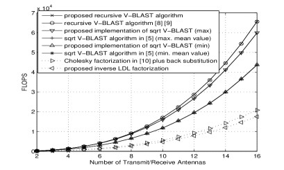
Figure 1: Complexity Comparison among the Presented Algorithms.

VI Conclusion

In this letter, the inverse LDM^T and LU factorizations are proposed for a matrix partitioned into $2\times 2$ blocks, which include the square-root and division free version. The proposed square-root and division free inverse LDM^T factorization is applied to compute the initial estimation error covariance matrix $\mathbf{Q}$ for the recursive V-BLAST algorithm, and is also applied to propose the square-root and division free implementation for the square-root V-BLAST algorithm in [5], where the wide-sense Givens rotation in [14] is utilized. With respect to the existing recursive V-BLAST algorithm [8, 9], the recursive V-BLAST algorithm with the initial $\mathbf{Q}$ computed by the proposed square-root and division free inverse LDM^T factorization requires about the same computational complexity, and can save $K-1$ divisions. With respect to the existing square-root V-BLAST algorithms [5, 6], the proposed square-root and division free V-BLAST algorithm requires about the same computational complexity, and can avoid the square-root and division operations.

References

• [1] G. J. Foschini and M. J. Gans, β€œOn limits of wireless communications in a fading environment when using multiple antennas”, Wireless Personal Commun., pp. 311-335, Mar. 1998.
• [2] P. W. Wolniansky, G. J. Foschini, G. D. Golden and R. A. Valenzuela, β€œV-BLAST: an architecture for realizing very high data rates over the rich-scattering wireless channel”, Proc. ISSSE 98, pp. 295-300, 1998.
• [3] B. Hassibi, β€œAn efficient square-root algorithm for BLAST”, IEEE ICASSP ’00, pp. 737-740, June 2000.
• [4] H. Zhu, Z. Lei, and F. P. S. Chin, β€œAn improved square-root algorithm for BLAST”, IEEE Signal Process. Lett., vol. 11, no. 9, pp. 772-775, Sep. 2004.
• [5] H. Zhu, W. Chen, B. Li, and F. Gao, β€œAn Improved Square-Root Algorithm for V-BLAST Based on Efficient Inverse Cholesky Factorization”, IEEE Trans. Wireless Commun., vol. 10, no. 1, Jan. 2011.
• [6] K. Pham and K. Lee, β€œLow-Complexity SIC Detection Algorithms for Multiple-Input Multiple-Output Systems”, IEEE Trans. on Signal Processing, pp. 4625-4633, vol. 63, no. 17, Sept. 2015.
• [7] J. Benesty, Y. Huang and J. Chen, β€œA fast recursive algorithm for optimum sequential signal detection in a BLAST system”, IEEE Trans. on Signal Processing, pp. 1722-1730, July 2003.
• [8] Y. Shang and X. G. Xia, β€œOn fast recursive algorithms for V-BLAST with optimal ordered SIC detection”, IEEE Trans. Wireless Commun., vol. 8, pp. 2860-2865, June 2009.
• [9] H. Zhu, W. Chen and F. She, β€œImproved Fast Recursive Algorithms for V-BLAST and G-STBC with Novel Efficient Matrix Inversion,” IEEE ICC 2009, Dresden, Germany, June 2009.
• [10] L. M. Davis, β€œScaled and decoupled Cholesky and QR decompositions with application to spherical MIMO detection”, IEEE WCNC, 2003.
• [11] E. N. Frantzeskakis and K. J. R. Liu, β€œA class of square root and division free algorithms and architectures for QRD-based adaptive signal processing”, IEEE Trans. on Signal Processing, Sep 1994.
• [12] G. H. Golub and C. F. Van Loan, Matrix Computations, Johns Hopkins University Press, Baltimore, MD, 3rd edition, 1996.
• [13] https://ww2.mathworks.cn/help/matlab/ref/inv.html?lang=en.
• [14] H. Zhu, W. Chen, and B. Li, β€œEfficient Square-Root and Division Free Algorithms for Inverse $LDL^{T}$ Factorization and the Wide-Sense Givens Rotation with Application to V-BLAST”, IEEE Vehicular Technology Conference (VTC), 2010 Fall, 6-9 Sept., 2010.
• [15] A. Burian, J. Takala, M. Ylinen, β€œA fixed-point implementation of matrix inversion using Cholesky decomposition”, IEEE International Symposium on MHS, Dec. 2003, Vol. 3, pp. 1431-1434.