Universal Stego Post-processing for Enhancing Image Steganography

Abstract

It is well known that the designing or improving embedding cost becomes a key issue for current steganographic methods. Unlike existing works, we propose a novel framework to enhance the steganography security via post-processing on the embedding units (i.e., pixel values and DCT coefficients) of stego directly. In this paper, we firstly analyze the characteristics of STCs (Syndrome-Trellis Codes), and then design the rule for post-processing to ensure the correct extraction of hidden message. Since the steganography artifacts are typically reflected on image residuals, we try to reduce the residual distance between cover and the modified stego in order to enhance steganography security. To this end, we model the post-processing as a non-linear integer programming, and implement it via heuristic search. In addition, we carefully determine several important issues in the proposed post-processing, such as the candidate embedding units to be modified, the direction and amplitude of post-modification, the adaptive filters for getting residuals, and the distance measure of residuals. Extensive experimental results evaluated on both hand-crafted steganalytic features and deep learning based ones demonstrate that the proposed method can effectively enhance the security of most modern steganographic methods both in spatial and JPEG domains.

I Introduction

Image steganography is a technique to hide secret message into cover images via modifying some image components in an imperceptible manner. On the contrary, image steganalysis aims to detect the existence of secret message hidden by image steganography. During the past decade, many effective steganography methods have been proposed with the development of the steganalytic techniques.

Image steganography can be divided into two categories, that is, spatial steganography and JPEG steganography. In modern research, both of them are usually designed under the framework of distortion minimization [1], in which the design of embedding cost is the key issue. Typically, the embedding cost tries to measure the statistical detectability of each embedding unit (i.e. pixel or DCT coefficient). The smaller the embedding cost, the more likely the corresponding unit will be modified during the subsequent operation of Syndrome-Trellis Codes (STCs) [2]. Up to now, there are many effective cost have been proposed in spatial domain. Most of them such as HUGO [3], WOW [4], S-UNIWARD [5], HILL [6] and MIPOD [7] adopt an additive cost, meaning that they assume the embedding impact for each unit is independent. Some methods such as CMD (Clustering Modification Directions) [8], Synch [9] and DeJoin [10] improve the existing additive cost via sequentially embedding message and updating the cost to synchronize the modification direction. These methods usually achieve better security performance since the mutual impacts of adjacent embedding units are taken into consideration. For JPEG steganography, the additive cost-based methods include UED [11], J-UNIWARD [5], UERD [12], BET [13], and the non-additive one includes BBC [14], which aims to preserve the spatial continuity at block boundaries. To enhance security, some other steganography methods aim to adjust existing costs via highlighting the details in an image [15, 16] or reassigning lower costs to controversial units [17, 18]. Recently, some deep learning techniques such as Generative Adversarial Network (GAN) [19] and adversarial example [20] have been applied in steganography. For instance, ASDL-GAN [21] and UT-GAN [22, 23] can learn costs that are directly related to the undetectability against the steganalyzer. ADV-EMB [24] and method [25] adjust the costs according to the gradients back-propagated from the target Convolutional Neural Network (CNN)-based steganalyzer.

Note that above steganography methods mainly focus on designing embedding costs, and usually employ the STCs to minimize the total costs in subsequent data hiding. However, most existing embedding costs seem empirical, which would not be effective to measure the statistical detectability of embedding units. In addition, minimizing the total costs using STCs would not always produce high security stegos. Unlike existing works, we propose a novel framework to enhance the security of current steganography methods both in spatial and JPEG domains via stego post-processing, which aims to reduce the residual distance between cover and modified stego. We firstly formulate the stego post-processing as a non-linear integer programming problem, and solve it using a heuristic search method - Hill Climbing. To achieve good security performance, the adaptive filters for obtaining image residuals and the distance measure are carefully designed. In addition, four acceleration strategies according to the characteristics of post-modification are considered to speed up our algorithm. Experimental results show that the proposed method can significantly enhance the security performance of the existing steganography methods, especially when the payloads and/or quality factors are large. Note that this paper is an extension of our previous work [26]. Compared to our preliminary work [26], the main differences of this paper are as follows: 1) Instead of using a fixed filter in [26] to obtain image residuals, in this paper, we carefully design multiple adaptive filters which can better suppress image content while preserve the artifacts left by data hiding; 2) The method in this extended version significantly accelerates the post-processing via restricting the position of modified units, the direction and amplitude of modification, and adopting a fast method for convolution; 3) More extensive experimental results and analysis are given in this paper. For instance, both conventional and deep learning steganalytic models are used for security evaluation. In addition to BOSSBase [27], other two public databases (i.e., BOWS2 [28] and ALASKA [29]) which include 90,005 images are used for evaluation. We provide more analysis on statistical characteristics of post-modification and the processing time. In addition, both spatial and JPEG steganographic methods are considered in this paper; 4) The extensive experimental results show that the proposed method can achieve higher security than the work [26].

Compared to those works (e.g. CMD [8], BBC [14], and methods [15, 16, 17, 18]) which also aim to enhance existing steganography methods, the main differences of the proposed method are as follows:

• First of all, almost all related works try to modify embedding costs of existing steganography during data hiding, while the proposed method tries to modify embedding units (pixel values or DCT coefficients) directly after the data hiding with the existing steganopgraphy is completed. Note that the early steganography OutGuess [30] divides the cover into two non-overlapping parts: one part for data hiding, the other part for histogram correction. From this point of view, OutGuess can be regarded as an enhanced steganography based on post-processing. However, the embedding capacity of OutGuess is significantly reduced since it has to reserve a relatively high proportion of embedding units for histogram correction. What is more, it can be easily detected by the modern steganalytic methods based on higher order statistics.

• The principle of related works is quite different. For instance, CMD aims at clustering modification directions and BBC aims at preserving the block boundary continuity, OutGuess [30] aims at preserving the histogram, while the proposed method aims at reducing the residual distance between cover and the resulting stego. Since the proposed method is performed on the stego, it is not contradictory to those steganographic works based on STC embedding. As shown in Section IV, most modern steganographic methods, such as MIPOD, CMD-HILL, J-UNIWARD and BET-HILL, can be further improved after using the proposed post-processing.

• Most existing works are usually designed under a special domain. For instance, the spatial steganographic methods such as MIPOD and CMD are difficult to be adopted in JPEG with satisfactory results. Similarly, those effective works for JPEG steganography may not effective in spatial domain. Comparatively, the proposed method is effective in both domains.

The rest of this paper is arranged as follows. Section II describes STCs and their robustness against post-modification. Section III describes the proposed framework. Section IV presents experimental results and discussions. Finally, the concluding remarks of this paper are given in Section V.

II Robustness Analysis of STCs

Most current steganographic methods are constructed under the framework of distortion minimization. After the embedding costs are carefully designed, some coding methods are then used to embed secret message into cover image in order to minimize the total cost. In practical applications, STCs is widely used in modern steganography methods both in spatial and JPEG domains. Since the extraction of hidden message after using the proposed method is related to STCs, we will give a brief overview of STCs and its robustness against post-modification in the following.

II-A Review of Syndrome-Trellis Codes

STC is one of the popular coding methods which is able to embed secret message into the cover image efficiently while approaching the optimal coding performance. It can be used to solve binary or non-binary embedding problem under the steganography framework of distortion minimization. For binary problem, the message embedding and extraction for spatial steganography can be formulated as follows:

$$Emb(X,m)=\arg\min_{P(Y)\in C(m)}D(X,Y)$$ (1)

$$Ext(Y)=\mathbb{H}P(Y)$$ (2)

where $Emb()$ is the function for data embedding. $Ext()$ is the function for message extraction. $X$ is a cover image. $Y$ is a stego image. $m$ is a secret message. $P$ is a parity function such as $P(Y)=Y\mod 2$. $\mathbb{H}$ is a parity-check matrix of a binary linear code $C$. $C(m)=\{z|\mathbb{H}z=m\}$ is the coset corresponding to syndrome $m$. STCs constructs the parity-check matrix $\mathbb{H}$ by placing a small submatrix $\hat{\mathbb{H}}$ along the main diagonal. The height of the submatrix $\hat{\mathbb{H}}$ is a parameter that can be used to balance the algorithm performance and speed. Using parity-check matrix $\mathbb{H}$ constructed in this way, equation (1) can be solved optimally by Viterbi algorithm with linear time and space complexity w.r.t. $n$, which is the dimension of $X$.

For the q-ary (q $>$ 2) embedding problem, STCs solves it efficiently via multi-layered construction. It decomposes the q-ary problem into a sequence of similar binary problem and then applies the above solution for binary problem. The q-ary problem can be solved optimally if each binary problem is solve optimally. Refer to [2] for more details of STC.

II-B Analysis of Robustness of STCs

From equation (2), the value of extracted message is determined by $\mathbb{H}$ and $P(y)$. In a covert communication, since $\mathbb{H}$ is fixed for a cover image, the message extraction completely relies on $P(y)$. Therefore, if there exists a modification matrix $\Delta$ such that $P(Y+\Delta)=P(Y)$, we can extract exactly the same secret message from $Y+\Delta$ and $Y$, which shows the robustness of STCs against the modification $\Delta$ in this case. Generally, image steganography embeds message into lower bits of the cover image for not introducing visually perceptible artifacts. Therefore, the parity function $P$ of q-ary STCs returns the $1^{st}$ to $k^{th}$ LSBs of the input image, where $k=\lceil\log_{2}q\rceil$. Based on this characteristic, q-ary STCs’ robustness against post-modification can be formulated as follows:

$$Ext(Y)=Ext(Y+\Delta),\quad\Delta_{ij}=2^{k}\times n_{ij},n_{ij}\in\mathcal{Z}$$ (3)

where $Y$ and $\Delta$ are matrices of the same size $n_{1}\times n_{2}$, $\Delta_{ij}$ denotes the $ij^{th}$ element of the modification matrix $\Delta$

Taking a stego image $Y$ obtained by ternary STCs (i.e. $q=3$) for example, in this case, $k=\lceil\log_{2}q\rceil=2$. $\Delta_{i,j}=2^{2}\times n_{ij}=4n_{ij}$, $n_{ij}\in\mathcal{Z}$. Therefore, we conclude that adding a multiple of 4 to any elements of the stego image will not confuse the message extraction at all.

III Proposed Framework and Method

In this section, we first describe the framework of stego post-processing, and then present some implementation details, including the selection of some important parameters and four strategies to speed up processing. Finally, we will give the full description of the proposed algorithm under this framework.

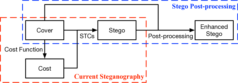
Figure 1: The framework of modern steganography vs. the proposed stego post-processing.

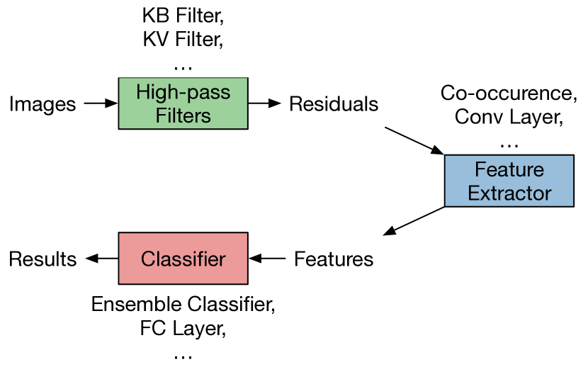
Figure 2: The framework of modern image steganalytic methods.

III-A Framework of Stego Post-processing

As shown in Fig. 1, the current steganography firstly designs costs for all embedding units of a cover image, and then uses STCs to embed secret message into cover to get the resulting stego. Quite different from the existing works, the proposed framework aims to enhance the steganography security via reducing image residual distance between cover and stego using stego post-processing. Since most current steganography methods, such as HILL [6] and UERD [12], employ ternary STCs for data embedding, the ternary case (i.e. $k=2$) is considered in our experiments. Please note that it is easy to extend our method for different $k$.

III-A1 Main Idea of Stego Post-processing

It is well known that the steganography will introduce detectable artifacts into image residuals, and thus most effective steganalyzers based on hand-crafted features (e.g. SRM [31], GFR [32]) and deep learning (e.g. Xu-Net [33], Ye-Net [34], and J-Xu-Net [35]) are mainly based on analyzing image residuals in spatial domain. As illustrated in Fig. 2, these steganalytic methods usually contain 3 components, that is, high-pass filters to obtain image residuals, feature extraction operator of image residuals and a classifier based on the features. Since the steganography signal is rather weak compared to image content, good high-pass filters can effectively suppress image content and improve the signal-to-noise ratio (note that for steganalysis, noise here is image content), which is very helpful for steganalysis. From this point of view, if the image residual distance between cover and modified stego image is smaller, the security performance is expected to be better. Therefore, the main idea of the proposed framework is to reduce such distance via stego post-processing. Combined with the robustness analysis on STCs in section II-B, the proposed stego post-processing can be formulated as the following optimization problem:

$$\underset{Z}{\text{minimize}} Dist(Res(Z),Res(X))$$ (4)

subject to $$Z=Y+2^{2}\times N,$$

$$N\in\mathcal{Z},$$

$$Z\in\mathcal{V}.$$

where $Res(X)$ denotes the image residual of image $X$ in spatial domain, $Dist(Res(Z),Res(X))$ denotes the distance between two image residuals $Res(Z)$ and $Res(X)$; $X$ is a cover image, $Y$ is a stego image obtained with an existing steganography method, $Z$ is a modified version of $Y$ with our post stego-processing; $N$ is an integer matrix; $\mathcal{V}$ denotes the available range of embedding units of $Z$. Taking spatial steganography for instance, every unit in $\mathcal{V}$ should be an integer in the range of $[0,255]$.

Note that the proposed framework tries to modify a resulting stego $Y$ obtained with an existing steganography method under the framework of distortion minimization, thus any modification on $Y$ will inevitably increase the total distortion. However, we expect that the steganography security would become better since the residual distance between cover $X$ and the resulting stego $Z$ is reduced after stego post-processing.

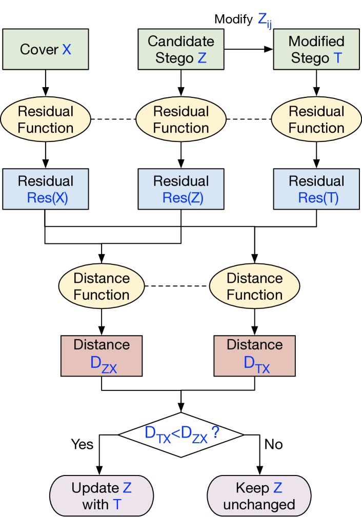
Figure 3: The proposed method to update a target embedding unit within a stego image.

III-A2 Implementation of the Framework

Since the modifications are limited on integers, and the distance function $Dist()$ is usually non-linear, the optimization problem described in the previous section is a non-linear integer programming, which is very hard to find the optimal solution. In our experiments, we employ a greedy algorithm, i.e., Hill Climbing, to find an approximate solution. Specifically, from an initial stego $Y$, we sequentially process the embedding units one by one to iteratively reduce its residual distance to cover $X$ until all embedding units are dealt with.

Fig. 3 illustrates how the proposed method updates a target embedding unit within a stego image. Let $X$ denote cover, $Z$ denote the candidate stego which is initialized as the stego $Y$ with an existing steganography method, $T$ denote the temporary variable for the modified version of $Z$ after changing a target unit $Z_{ij}$ according to the rule described in section II (i.e. $T=Z,T_{ij}=T_{ij}+2^{2}\times n,n\in\mathcal{Z}$). By doing so, we can assure that the secret messages extracted from $Z$ and $Y$ are exactly the same after modification. To determine whether the modified stego $T$ is better than the candidate one $Z$, we firstly apply $Res()$ function on cover image $X$ and two stego images $Z$, $T$, and get the corresponding image residuals $Res(X)$, $Res(Z)$ and $Res(T)$ separately. And then we calculate the distance between the residual of cover $Res(X)$ and the two image residuals $Res(Z)$ and $Res(T)$ separately according to a certain $Dist()$ function, denoted as $D_{ZX}$ and $D_{TX}$. Finally, we will update the candidate stego $Z$ as the temporary $T$ if $D_{ZX}>D_{TX}$, otherwise we keep $Z$ unchanged.

We repeat the above operations for all embedding units, and the whole pseudo-code of the proposed framework is illustrated in Algothrim 1. The inputs of the algorithm are cover $X$ and the corresponding stego $Y$ using an existing steganography method. The algorithm first initializes the candidate stego $Z$ as $Y$, and then updates $Z$ using three loops. In the first loop (i.e. line 6 - 22), it traverses all the embedding units row by row. In the second loop (i.e. line 7 - 21), it considers the direction of post-modification to an embedding unit (positive $+$ or negative $-$). In the third loop (i.e. line 8 - 20), it considers different amplitudes of post-modification to an embedding units (e.g. $4,8,12,\cdots$). After the three loops, the algorithm finally outputs a modified stego $Z$, which usually has smaller residual distance compared with the input stego $Y$.

Algorithm 1 Pseudo-code for the stego post-processing. $X,Y,Z$ denote the values are of size $n_{1}\times n_{2}$. The for loop in Line 6 traverses all embedding units row by row.

1:Input: cover image $X$; stego image $Y$

2:Output: modified stego image $Z$

3:Initialize $Z=Y$

4:$R_{X}=Res(X)$

5:$R_{Z}=Res(Z)$

6:for  $i\in\{1,...,n_{1}\},\ j\in\{1,...,n_{2}\}$  do

7:     for  $s\in\{+4,-4\}$  do

8:         while  $Z_{ij}+s\in\mathcal{V}$  do

9:              $T=Z$

10:              $T_{ij}=Z_{ij}+s$

11:              $R_{T}=Res(T)$

12:              $D_{TX}=Dist(R_{T},R_{X})$

13:              $D_{ZX}=Dist(R_{Z},R_{X})$

14:              if $D_{TX}<D_{ZX}$  then

15:                  Update $Z_{ij}=T_{ij}$

16:                  Update $R_{Z}=R_{T}$

17:              else

18:                  break

19:              end if

20:         end while

21:     end for

22:end for

23:return $Z$

III-A3 Hyper-Parameters

The residual function $Res()$ in Algorithm 1 is the key issue that would significantly affect the security performance of the proposed framework. In the following, we will discuss the design of adaptive filter.

As described in section III-A1, most modern steganalytic features are mainly derived from image residuals. Thus, the selection of high-pass filters is very important for steganalysis. Until now, there are many available filters in existing works, such as various filters in SRM [31] and GFR [32]. Note that these filters are fixed for all images. Inspired from [36], we employ an adaptive way to learn high-pass filters for each image. Specifically, we first compute the convolution of the image with a prediction filter whose center element is 0, which amounts to predicting target pixels via their surrounding pixels; and then we determine the elements in the prediction filter by minimizing the mean square error between the predicted pixels and actual ones via lease squares; finally, we set the center of prediction filter as -1 to obtain the final filter, which calculate the residual between the predicted and actual values. Different from work [36] which learns a filter of size $w\times w$ ($w>2$) with symmetry constraint, we first learn a base filter of size $1\times w$ without symmetry constraint for any given image and its transposed version. Thus, the resulting basic filter (denoted as $B$) is a predictor of horizontal direction while its transposed version $B^{T}$ is a predictor of vertical direction. And then we get the outer product of $B$ and $B^{T}$, denoted as $B\otimes B^{T}$, which can calculate the residual based on the prediction of both horizontal and vertical directions. In our method, we can obtain different residual functions via the combination of the elements in set $\{B,B^{T},B\otimes B^{T}\}$ with different size $w$. Based on our experiments, we finally select the filters $\{B,B^{T},B\otimes B^{T}\}$ of size 7 for spatial steganography while filters $\{B,B^{T}\}$ of size 3 for JPEG steganography. Please note that we take into account several residuals by summing them up. More experimental results on the hyper-parameter selection are shown in section IV-A.

In Algorithm 1 (line 12-13), the distance function $Dist()$ is used to measure the residual distance between cover and stego. Different distances will lead to different post-modification, and thus affect security performance. We have tested several typical distance measures, including Manhattan, Euclidean, Chebychev and Hamming, and found that the Manhattan distance usually performs well on various steganography methods in both spatial and JPEG domains. Thus, we employ the Manhattan distance as follows in our experiments.

$$d(p,q)=||p-q||_{1}=\sum_{i=1}^{n}|p_{i}-q_{i}|$$ (5)

where $p=(p_{1},p_{2},...,p_{n})$, $q=(q_{1},q_{2},...,q_{n})$.

III-B Acceleration Strategies

Several issues would significantly affect the processing time of the proposed Algorithm 1. First of all, there are three nested loops. The first loop will traverse all embedding units of the input stego $Y$. Taking an image of size $512\times 512$ for example, there are totally 262144 ($=512\times 512$) units to be dealt with. For each unit, two directions (i.e. positive or negative in the second loop) and different modification amplitudes (i.e. 4, 8, $\ldots$, in the third loop) need to be considered. If we can reduce the iteration number of these loops, the algorithm speed will be improved. Furthermore, the filtering operation to get image residuals in the innermost loop is time-consuming. As a result, a fast method for filtering is needed. In the following sections, we will describe four acceleration strategies separately.

III-B1 Restriction on Position of Post-Modification

To reduce the number of embedding units to be dealt with in the first loop, we conduct experiment to report the post-modification rate in the set of units modified with steganography. Table I and Table II show the average results on 10,000 images from BOSSBase [27] for steganography methods in spatial and JPEG domains. From Tables I and II, we observe that for those embedding units modified by the stego post-processing, more of them are located at the small set of the units modified with steganography. Taking S-UNIWARD for instance, over 65% of post-modification are located at the set of units modified with steganography, which occupies only 7.39% of all units. Since the steganography modification rate is relatively lower in the experiment (less than 11% for spatial steganography for payload 0.4 bpp, and less than 4% for JPEG steganography for payload 0.4 bpnz), we consider dealing with those embedding units that have been previously modified with the steganography while skipping most unchanged units.

TABLE I: The post-modification rate in the set of units modified with steganography (%) evaluated on different spatial steganography methods (0.4 bpp).

S-UNI	MIPOD	HILL	CMD-HILL	Average
65.18	66.31	65.93	65.56	65.75

TABLE II: The post-modification rate in the set of units modified with steganography (%) evaluated on different JPEG steganography methods (0.4 bpnz).

QF	J-UNI	UERD	BET-HILL	Average
75	68.18	52.26	50.22	56.89
95	65.30	54.67	53.70	57.89

III-B2 Restriction on Direction of Post-Modification

In the previous section, we limited the post-modification to be performed on those embedding units which have been modified with steganography. To speed up the second loop, we will analyze the relationship between the directions of post-modification and steganography modification. We consider the post-modification that locate in the units that has modified by steganography and report the ratio of the post-modifications whose direction is opposite to that of steganography modifications in Table III and Table IV. The two tables show the average results on 10,000 images from BOSSBase [27] in different cases. From the two tables, we observe that the direction of post-modification is usually contrary to that of steganography modification. On average, such ratio is over 98% and over 86% for spatial and JPEG steganography separately. In our method, therefore, we will limit the direction of post-modification. This property is reasonable since the detectable artifacts left by steganography usually become more obvious when the direction of post-modification is the same as that of steganography modification.

TABLE III: The ratio of the post-modifications whose direction is opposite to that of steganography modifications (%) evaluated on different spatial steganography methods (payload 0.4 bpp).

S-UNI	MIPOD	HILL	CMD-HILL	Average
99.59	98.91	99.01	96.28	98.45

TABLE IV: The ratio of the post-modifications whose direction is opposite to that of steganography modifications (%) evaluated on different JPEG steganography methods (payload 0.4 bpnz).

QF	J-UNI	UERD	BET-HILL	Average
75	95.76	92.42	89.53	92.57
95	90.70	85.11	83.54	86.45

III-B3 Restriction on Amplitude of Post-Modification

In section II-B, we showed that adding a multiple of 4 to any embedding unit of the stego image would not confuse the message extraction. However, most existing literatures have shown that the security performance of steganography usually becomes poorer when the steganography modification becomes relatively larger. To enhance steganography security, we expect that most amplitudes of the post-modification are the smallest ones, i.e. 4, for the ternary STCs. According to our experiments on 10,000 images from BOSSBase [27], we observe that the amplitude of 100% and over 98% post-modification is equal to 4 for spatial (i.e. S-UNIWARD, MIPOD, HILL, CMD-HILL) and JPEG (i.e. J-UNIWARD, UERD, BET-HILL) steganography methods separately, which fits our expectations very well. Therefore, we limit the amplitude for the post-modification to 4 in our method.

III-B4 Efficient Convolution

In the three previous subsections, we try to reduce the loop count of the three loops in Algorithm 1 separately. In this section, we will speed up the key operation - i.e. the $Res()$ function to obtain image residual in the innermost loop (i.e. line 11) in Algorithm 1.

In section III-A3, we determine to employ several adaptive convolution filters with a smaller size (i.e. $w=3$ or $w=7$, which is significantly smaller than the image size $n_{1}$ and $n_{2}$, i.e. $n_{1}=n_{2}=512$ or $256$ in our experiments) to update image residual of temporary stego $T$. Please note that the convolution is linear and it just affects a small region of embedding units that around the filter center. Thus, there is no need to perform the convolution on the whole temporary stego $T$ to obtain its residual, since just an element within $T$ is different from the candidate stego $Z$ (refer line 9-10 in Algorithm 1). An equivalent and efficient method is employed in our method. When the image residual of $Z$ is available (i.e. $R_{Z}$), the image residual of $T$ can be calculated based on the following formula:

$$R_{T} =conv(T,F)=conv(Z\pm\delta_{ij}\times 4,F)$$ (6)

$$=conv(Z,F)\pm conv(\delta_{ij},F)\times 4$$

$$=R_{Z}\pm conv(\delta_{ij},F)\times 4$$

where $\delta_{ij}$ is a matrix of the same size $n_{1}\times n_{2}$, and its elements are all 0 except that the element at position $(i,j)$ is 1.

Due to the characteristic of matrix $\delta_{ij}$, it is very fast to get the $R_{T}$ via modifying a small region corresponding to the position $(i,j)$ within $R_{Z}$, that is, a region of size $w\times w$ for spatial steganography or a region of size $(w+7)\times(w+7)$ for JPEG steganography. By doing so, we can obtain over 500 times acceleration both in spatial and JPEG steganography based on our experiments.

III-C The Proposed Method

The pseudo-code for the proposed stego post-processing is illustrated in Algorithm 2. Note that the source code of the Algorithm 2 can be available at GitHub. According to the first three acceleration strategies, we observe that only one loop (i.e. line 6-20 in Algorithm 2) is remaining here compared to Algorithm 1, and most embedding units in this loops will be skipped (i.e. line 10-12 in Algorithm 2). According to the analysis in Section III-B - 4), the execution time is unbearable without using the fast method for obtaining temporary image residual . Thus the fast method is employed in both Algorithm 1 and Algorithm 2. For a fair comparison, both algorithms are implemented with Matlab and on the same server with CPU Intel Xeon Gold 6130. The processing time and the security performance of two algorithms would be evaluated in the following.

Algorithm 2 Pseudo-code for the stego post-processing. Images $X,Y,Z$ are of size $n_{1}\times n_{2}$. $F$ is the adaptive filter generated based on predictor learned from $X$. The for loop in Line 6 traverses all embedding units row by row.

1:Input: cover image $X$; stego image $Y$

2:Output: enhanced stego images $Z$

3:Initialize $Z=Y$

4:$R_{X}=conv(X,F)$

5:$R_{Z}=conv(Z,F)$

6:for  $i\in\{1,...,n_{1}\},\ j\in\{1,...,n_{2}\}$  do

7:     $s=(X_{ij}-Y_{ij})\times 4$

8:     $T=Z$

9:     $T_{ij}=Z_{ij}+s$

10:     if  $s==0$ or $T_{ij}\notin\mathcal{V}$  then

11:         continue

12:     end if

13:     $R_{T}=$ Update a small region of $R_{Z}$

14:     $D_{ZX}=\sum|R_{Z}-R_{X}|$

15:     $D_{TX}=\sum|R_{T}-R_{X}|$

16:     if $D_{TX}<D_{ZX}$  then

17:         Update $Z_{ij}=T_{ij}$

18:         Update $R_{Z}=R_{T}$

19:     end if

20:end for

21:return $Z$

III-C1 Comparison on Processing Time

In this experiment, we will compare the processing time of the algorithm before and after using the first three acceleration strategies. Four spatial steganography methods and three JPEG steganograpy methods are considered . The comparative results are shown in Table V and Table VI. From the two tables, we observe that the processing time of the proposed method (i.e. Algorithm 2) is significantly shorter than the original one (i.e. Algorithm 1). On average, we gain over 12 and 9 times speed improvement for the spatial and JPEG steganography separately.

TABLE V: Processing time (s) for Algorithm 1 and Algorithm 2 in spatial domain (0.4 bpp).

	S-UNI	MIPOD	HILL	CMD-HILL	Average
Algorithm 1	3.75	3.72	3.75	3.72	3.74
Algorithm 2	0.27	0.29	0.29	0.33	0.30

TABLE VI: Processing time (s) for Algorithm 1 and Algorithm 2 in JPEG domain (0.4 bpnz).

QF	Strategy	J-UNI	UERD	BET-HILL	Average
75	Algorithm 1	4.65	4.66	4.64	4.65
	Algorithm 2	0.50	0.49	0.49	0.49
95	Algorithm 1	4.83	4.85	4.81	4.83
	Algorithm 2	0.54	0.53	0.53	0.53

III-C2 Comparison on Security Performance

In this experiment, we will compare the security performances of Algorithm 1 and Algorithm 2. The experimental results are shown in Table VII and Table VIII. From the two tables, we observe that both algorithms can enhance the steganography security in all cases. Although we have significantly simplified the Algorithm 1 for acceleration, the performance of Algorithm 2 would not drop. On the contrary, it is able to outperform Algorithm 1 slightly on average.

TABLE VII: Detection accuracies (%) for Algorithm 1 and Algorithm 2 in spatial domain (0.4 bpp). The steganalytic feature set is SRM. In all following tables, the value with an asterisk (*) denotes the best result.

	S-UNI	MIPOD	HILL	CMD-HILL	Average
Baseline	79.68	75.66	75.72	70.06	75.28
Algorithm 1	78.34	72.83*	72.96	69.35	73.37
Algorithm 2	78.31*	73.19	72.42*	68.93*	73.21*

TABLE VIII: Detection accuracies (%) for Algorithm 1 and Algorithm 2 in JPEG domain (0.4 bpnz). The steganalytic feature set is GFR.

QF	Strategy	J-UNI	UERD	BET-HILL	Average
75	Baseline	89.66	89.59	87.13	88.79
	Algorithm 1	88.81	88.15	84.76	87.24
	Algorithm 2	88.54*	87.48*	84.59*	86.87*
95	Baseline	72.79	76.00	69.22	72.67
	Algorithm 1	72.26	73.72	66.31*	70.76
	Algorithm 2	71.75*	73.46*	66.88	70.70*

IV Experimental Results and Discussions

In our experiments, we collect 10,000 gray-scale images of size $512\times 512$ from BOSSBase [27], and randomly divide them into two non-overlapping and equal parts, one for training and the other for testing. Like most existing literatures, we use the optimal simulator for data embedding. Four typical spatial steganography methods (i.e. S-UNIWARD [5], MIPOD [7], HILL [6] and CMD-HILL [8]) and three typical JPEG steganography methods (i.e. J-UNIWARD [5], UERD [12] and BET-HILL [13]) are considered. The spatial steganalytic detectors include two conventional feature sets (i.e. SRM [31], maxSRM [37]) and a CNN-based one (i.e. Xu-Net [33]). Similarly, the JPEG steganalytic detectors also include two conventional ones (i.e. GFR [32], SCA-GFR [38] ) and a CNN-based one (i.e. J-Xu-Net [35]). The ensemble classifier [39] is used for conventional steganalytic features.

IV-A Hyper-Parameter Selection

The residual function $Res()$ is the key issue in the proposed algorithm that will significantly affect the security performance. We employ several adaptive filters to get image residuals. In this section, we try to select proper hyper-parameter about the adaptive filters, including the adaptive filter set and the size of basic filter $B$.

TABLE IX: Detection accuracies (%) for different filter sets in spatial steganography (0.4 bpp). In all following tables, the underlined value denotes the pooper result compared to the baseline steganography.

Filter Set	S-UNI	MIPOD	HILL	CMD-HILL	Average
Baseline	79.68	75.66	75.72	70.06	75.28
$\{B\otimes B^{T}\}$	78.82*	74.58	73.87	70.37	74.41
$\{B,B^{T}\}$	79.42	75.69	75.13	70.02	75.07
$\{B,B^{T},B\otimes B^{T}\}$	79.16	74.37*	73.75*	69.95*	74.31*

TABLE X: Detection accuracies (%) for different filter sets in JPEG steganography (0.4 bpnz).

QF	Filter Set	J-UNI	UERD	BET-HILL	Average
75	Baseline	89.66	89.59	87.13	88.79
	$\{B\otimes B^{T}\}$	94.97	95.43	92.99	94.46
	$\{B,B^{T}\}$	88.54*	87.48*	84.59	86.87*
	$\{B,B^{T},B\otimes B^{T}\}$	88.56	87.67	84.54*	86.92
95	Baseline	72.79	76.00	69.22	72.67
	$\{B\otimes B^{T}\}$	80.56	85.42	75.81	80.60
	$\{B,B^{T}\}$	71.75*	73.46*	66.88	70.70*
	$\{B,B^{T},B\otimes B^{T}\}$	72.09	73.80	66.67*	70.85

TABLE XI: Detection accuracies (%) for different sizes of basic filter $B$ for spatial steganography (0.4 bpp). The filter set is $\{B,B^{T},B\otimes B^{T}\}$. The steganalytic feature set is SRM.

Size	S-UNI	MIPOD	HILL	CMD-HILL	Average
Baseline	79.68	75.66	75.72	70.06	75.28
3	79.16	74.37	73.75	69.95	74.31
5	78.28*	73.32	72.46	69.33	73.35
7	78.31	73.19*	72.42*	68.93*	73.21*
9	78.37	73.29	73.15	69.22	73.51

TABLE XII: Detection accuracies (%) for different sizes of basic filter $B$ for JPEG steganography (0.4 bpnz). The filter set is $\{B,B^{T}\}$. The steganalytic feature set is GFR.

QF	Size	J-UNI	UERD	BET-HILL	Average
75	Baseline	89.66	89.59	87.13	88.79
	3	88.54*	87.48*	84.59*	86.87*
	5	88.87	87.82	84.95	87.21
	7	88.81	87.99	85.35	87.38
	9	88.89	88.06	85.33	87.43
95	Baseline	72.79	76.00	69.22	72.67
	3	71.75*	73.46*	66.88	70.70*
	5	72.09	73.92	66.81*	70.94
	7	72.04	73.99	66.90	70.98
	9	72.34	74.17	66.90	71.14

TABLE XIII: Detection accuracies (%) for different steganography methods in spatial domain. In all following tables, we name the enhanced version of some steganography such as “A” with the proposed Stego Post-Processing as “A-SPP” for short.

Steganography	SRM					maxSRMd2					Xu-Net
	0.1	0.2	0.3	0.4	0.5	0.1	0.2	0.3	0.4	0.5	0.1	0.2	0.3	0.4	0.5
S-UNI	60.09	68.29	74.74	79.68	83.61	63.72	70.71	76.58	80.69	84.36	55.72	64.86	73.62	78.60	82.72
S-UNI-SPP	59.76*	67.55*	73.27*	78.31*	82.22*	63.31*	70.09*	75.16*	79.17*	82.75*	55.24*	63.71*	70.66*	75.37*	79.73*
MIPOD	58.25	65.68	71.44	75.66	80.20	60.77	67.37	72.92	77.41	81.34	58.06	65.52	71.11	75.66	80.43
MIPOD-SPP	58.37	63.83*	69.11*	73.19*	77.52*	59.36*	65.21*	70.15*	73.79*	78.33*	56.98*	62.38*	66.80*	71.36*	75.23*
HILL	56.65	64.14	70.44	75.72	79.67	62.43	69.32	73.72	78.30	81.92	58.04	65.50	71.40	77.26	80.23
HILL-SPP	56.09*	62.60*	67.68*	72.42*	76.47*	60.82*	66.82*	71.48*	75.72*	79.23*	56.29*	62.08*	66.92*	71.36*	75.50*
CMD-HILL	55.09	60.53	65.86	70.06	74.41	59.79	65.54	69.74	73.35	76.46	54.81	60.19	64.66	69.64	73.39
CMD-HILL-SPP	54.55*	60.13*	64.95*	68.93*	72.73*	59.40*	64.42*	68.81*	71.83*	75.50*	54.39*	59.07*	62.65*	67.44*	70.25*

TABLE XIV: Detection accuracies (%) for different steganography methods in JPEG domain.

QF	Steganography	GFR					SCA-GFR					J-Xu-Net
		0.1	0.2	0.3	0.4	0.5	0.1	0.2	0.3	0.4	0.5	0.1	0.2	0.3	0.4	0.5
75	J-UNI	59.03	71.00	81.82	89.66	94.50	64.33	76.91	85.94	91.75	95.47	65.28	77.66	86.13	91.72	95.01
	J-UNI-SPP	59.06	70.92*	81.23*	88.54*	93.46*	63.72*	76.36*	85.07*	90.87*	94.65*	65.23	77.53*	85.97*	91.46*	94.57*
	UERD	60.42	72.46	82.27	89.59	94.14	70.36	82.17	88.91	93.17	95.88	77.44	88.04	93.01	96.13	97.46
	UERD-SPP	59.60*	71.52*	81.11*	87.48*	92.54*	70.07*	81.08*	88.04*	92.10*	94.83*	77.06*	88.18	92.58*	95.95*	97.58
	BET-HILL	58.26	69.12	78.96	87.13	92.10	65.19	76.98	86.11	92.01	95.58	65.63	77.70	84.88	90.43	95.20
	BET-HILL-SPP	57.82*	67.58*	77.04*	84.59*	90.42*	64.08*	75.22*	83.85*	89.73*	93.59*	64.28*	76.62*	83.27*	89.57*	93.73*
95	J-UNI	52.41	57.92	65.15	72.79	80.63	53.59	59.94	67.21	73.90	80.00	50.26	57.88	66.43	73.38	79.03
	J-UNI-SPP	52.31*	57.66*	64.55*	71.75*	78.98*	53.52*	59.47*	65.98*	72.65*	78.27*	50.08*	57.72*	65.34*	72.42*	79.18
	UERD	54.18	60.62	68.49	76.00	82.77	59.33	67.89	74.57	80.53	85.44	50.12	73.37	82.39	88.97	92.79
	UERD-SPP	54.11*	60.01*	66.66*	73.46*	79.68*	59.06*	66.81*	72.85*	77.93*	82.65*	50.04*	72.74*	82.30*	88.17*	92.12*
	BET-HILL	52.24	56.75	62.30	69.22	75.59	54.14	59.47	65.36	71.73	77.81	50.47	58.49	65.36	73.01	80.00
	BET-HILL-SPP	52.06*	56.21*	61.22*	66.88*	72.86*	53.42*	58.19*	63.39*	69.18*	75.04*	49.90*	56.58*	64.09*	72.60*	78.07*

IV-A1 Adaptive Filter Set

As described in section III-A3, we first learn a basic filter $B$ for each image, and then produce two filters via transpose and outer product, and then we obtain three adaptive filters, that is, $B$, $B^{T}$ and $B\otimes B^{T}$. For simplification, three combinations of above filters are evaluated, that is, $\{B\otimes B^{T}\}$, $\{B,B^{T}\}$ and $\{B,B^{T},B\otimes B^{T}\}$. In addition, the filter size of $B$ is fixed as 3 in this experiment, and the steganalytic features SRM and GFR are used for security evaluation for the spatial (0.4 bpp) and JPEG steganography (0.4 bpnz) separately. The detection accuracies evaluated on test set are shown in Table IX and Table X. From Table IX, we observe that the three filter sets can improve the security performance of the four spatial steganography methods except using the filter $\{B\otimes B^{T}\}$ on CMD-HILL. On average, the set $\{B,B^{T},B\otimes B^{T}\}$ achieves the best performance, and it gains an average improvement of 0.97% compared to the baseline steganpgraphy. From Table X, we observe $\{B,B^{T}\}$ and $\{B,B^{T},B\otimes B^{T}\}$ can improve the security performance while $\{B\otimes B^{T}\}$ will significantly drop the performance. On average, the filter set $\{B,B^{T}\}$ performs the best and it achieves an improvement of around 1.90% for both quality factors. The above results show that different adaptive filter sets have a great influence on security performance. The filter sets $\{B,B^{T},B\otimes B^{T}\}$ and $\{B,B^{T}\}$ usually perform the best in spatial and JPEG domain separately.

IV-A2 Size of Basic Filter $B$

In previous section, we fixed the size of basic filter $B$ as 3, and selected the proper filter set for spatial and JPEG steganography separately. In this section, we first fixed the selected filter set, and evaluate their performances with different sizes of the basic filter $B$, including $w=3,5,7,9$. The detection accuracies are shown in Table XI and Table XII. From the two tables, we observe that the four filter sizes can improve the performance of various steganography methods in both spatial and JPEG domains. In spatial domain, the average performance becomes the best when the size of $B$ is 7 instead of 3, which will further gain an improvement of 1.10%. In JPEG domain, the proper size of $B$ is still 3 based on our experiments.

We should note that the hyper-parameter determined previously is just a suboptimal solution. Due to time constraint, we probably find a better solution via brute force method according to several important issues, such as the combinations of adaptive filters with different sizes, the specific steganography with a given payload, and the steganalytic models under investigation and so on. For simplicity, we just apply the filter set $\{B,B^{T},B\otimes B^{T}\}$ with filter size $w=7$ for spatial steganography, and the filter set $\{B,B^{T}\}$ with filter size $w=3$ for JPEG steganography for all embedding payloads and steganalytic models in the following section.

IV-B Steganography Security Evaluation

In this section, we will evaluate the security performance on different steganography methods for different payloads ranging from 0.1 bpp/bpnz to 0.5 bpp/bpnz. Three different steganalyzers in spatial domain, including SRM [31], maxSRM [37], and Xu-Net [33], and three steganalyzers in JPEG domain, including GFR [32], SCA-GFR [38], and J-Xu-Net [35], are used for security evaluation. The average detection accuracies on test set are shown in Table XIII and Table XIV. From the two tables, we obtain the three following observations:

• Almost in all cases, the proposed method can effectively improve the steganography security both in spatial and JPEG domains. The improvement usually increases with increasing embedding payload.

• In spatial domain, we can achieve greater improvements on MIPOD and HILL compared to S-UNIWARD and CMD-HILL. Taking the payload of 0.5 bpp for instance, we obtain about 3% improvement on both MIPOD and HILL, while less than 2% for two other steganography methods under two hand-crafted steganalytic feature sets, i.e. SRM and maxSRM. Furthermore, the proposed method seems more effective to the CNN-based steganalyzer (i.e. Xu-Net). For instance, we can obtain about 5% improvement for MIPOD and HILL for the payload of 0.5 bpp, which is a significant improvement on current steganography methods.

  

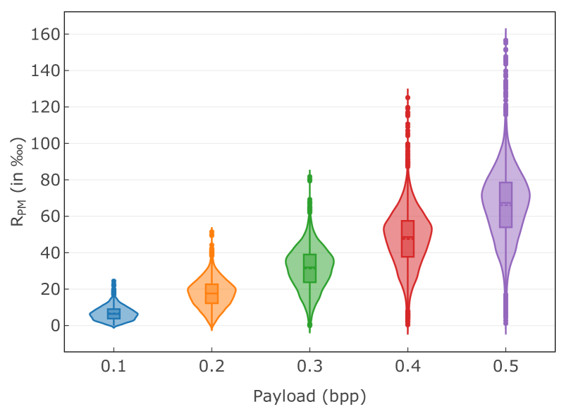
  (a) HILL

  

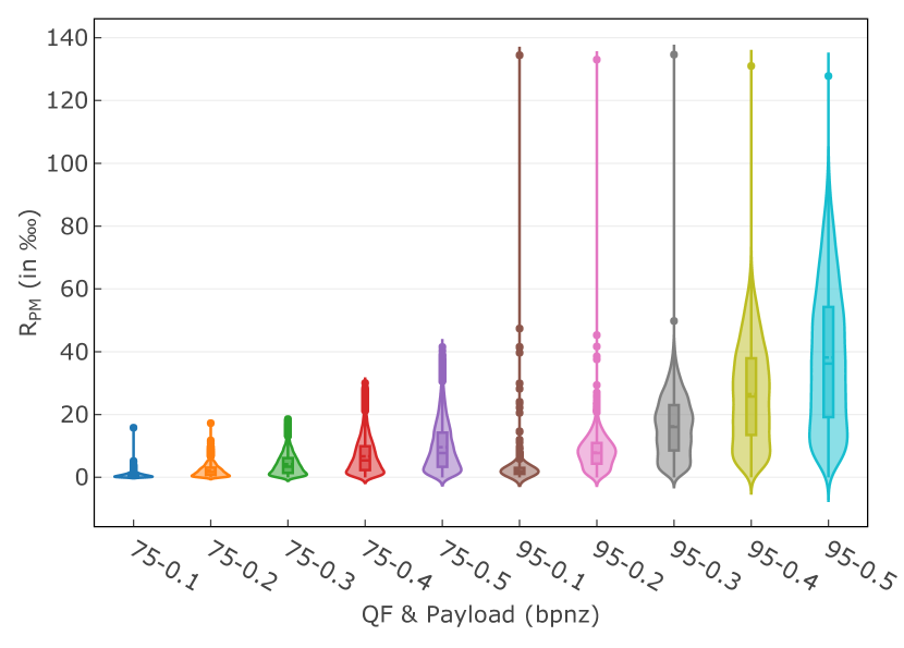
  (b) BET-HILL

  Figure 4: The violin plots of the Post-Modification Rates for HILL and BET-HILL

• In JPEG domain, the proposed method can gain more improvement on UERD and BET-HILL compared to J-UNIWARD. Taking the payload 0.5 bpnz and $QF=95$ for instance, it obtain an improvement of about 3% for both UERD and BET-HILL under the steganalytic feature GFR, while only 1.65% for J-UNIWARD. In addition, the proposed method seems less effective to CNN-based steganalyzer (i.e. J-Xu-Net) compared to the hand-crafted feature sets. In some cases, the security will drop slightly (less than 0.15%) after using the proposed method.

IV-C Analysis on Post-Modification

In this section, we will analyze some statistical characteristics on the post-modification with our method, including the modification rate and its relation to the density of steganography modification.

TABLE XV: Post-Modification Rate (‱) for steganography methods in spatial domain.

Steganography	0.1	0.2	0.3	0.4	0.5
S-UNI	3.81	11.21	21.30	33.92	48.89
MIPOD	3.26	12.87	27.14	45.17	66.34
HILL	6.64	17.53	31.30	47.54	66.09
CMD-HILL	2.67	7.44	13.81	21.91	31.78

TABLE XVI: Post-Modification Rate (‱) for steganography methods in JPEG domain.

QF	Steganography	0.1	0.2	0.3	0.4	0.5
75	J-UNI	0.37	1.42	3.07	5.21	7.87
	UERD	0.39	1.52	3.28	5.59	8.41
	BET-HILL	0.66	2.11	4.19	6.64	9.59
95	J-UNI	1.33	5.73	13.13	23.00	34.74
	UERD	1.84	7.16	15.48	26.09	38.48
	BET-HILL	2.21	7.87	16.24	26.53	38.23

IV-C1 Post-Modification Rate

We define the post-modification rate as follows:

$$R_{PM}=\frac{|Z\not=Y|}{|Y|}=\frac{|Z\not=Y|}{|X|}$$ (7)

where $X,Y,Z$ denote the set of embedding units in cover, stego, and the modified version with the proposed method separately. Note that $|X|=|Y|=|Z|$ since the number of embedding units is the same for the three images. Table XV and Table XVI show the average results evaluated on 10,000 images from BossBase. From the two tables, we observe that $R_{PM}$ will increase with increasing embedding payloads, and $R_{PM}$ is usually less than 67‱ and 39‱ for spatial and JPEG steganography separately even the embedding payload is as high as 0.5bpp / 0.50bpnz.

Fig. 4 shows the violin plots of $R_{PM}$ for HILL and BET-HILL in different cases. From the two figures, we observe that the median number of $R_{PM}$ usually increases with increasing payload. Even when the payload is as high as 0.5 bpp / 0.5 bpnz, the median number of $R_{PM}$ is less than 80‱ / 40‱, which means that we can achieve great improvement (refer to Table XIII and Table XIV) via just modifying a tiny fraction of embedding units for any given stego images $Y$.

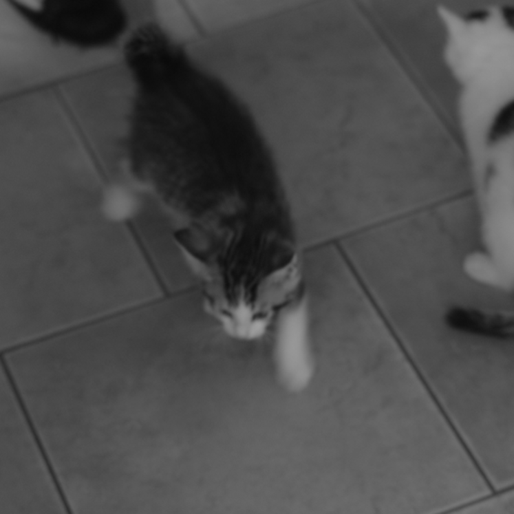
(a) No.7353

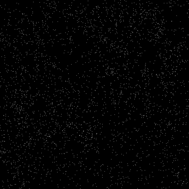
(b) Steganography Modification

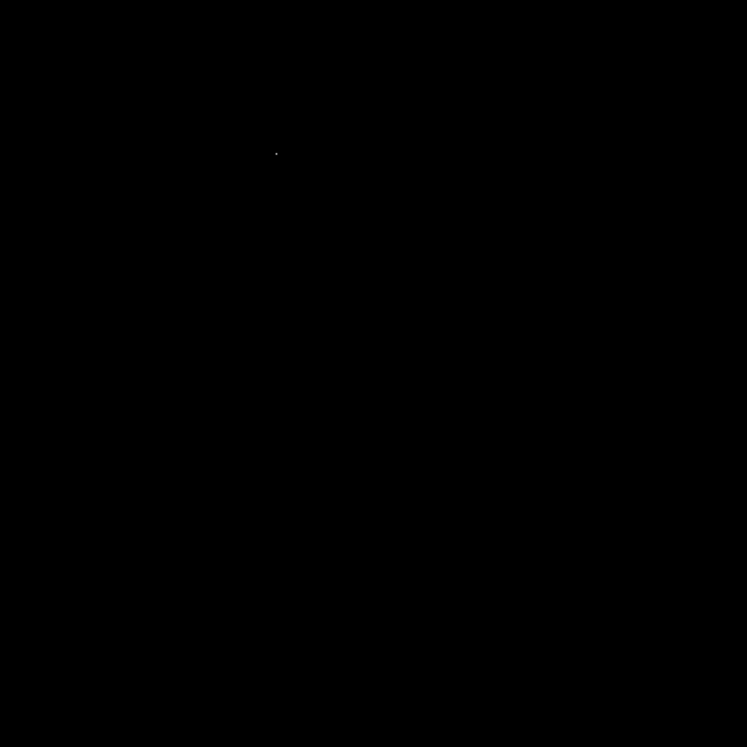
(c) Post-Modification

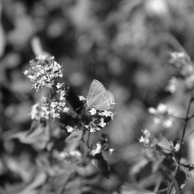
(d) No.1265

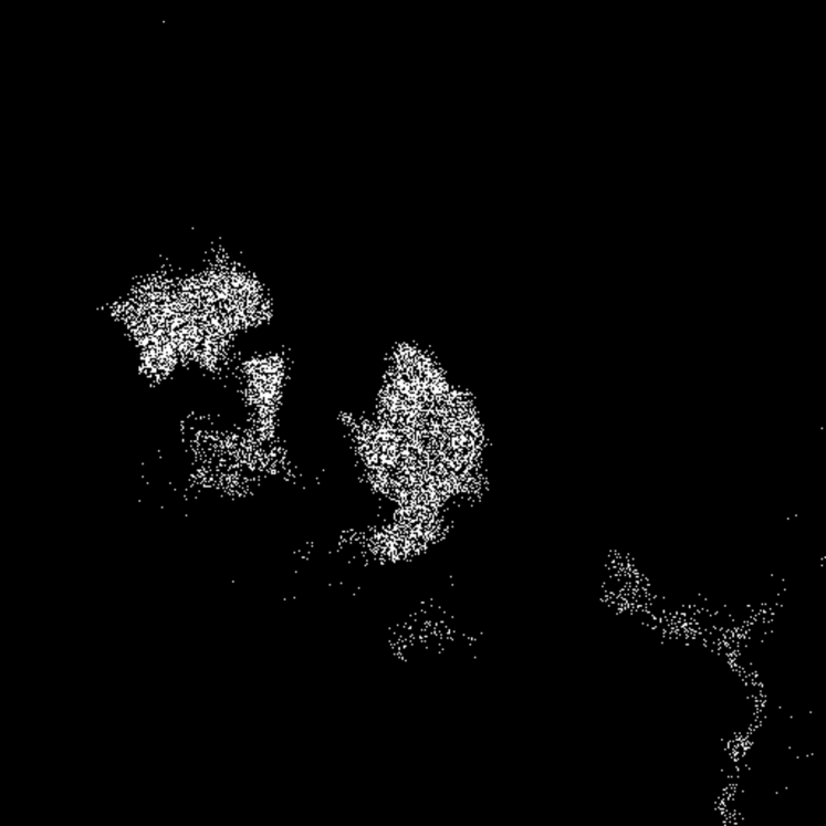
(e) Steganography Modification

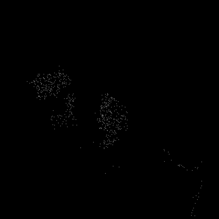
(f) Post-Modification

Figure 5: Steganography modification using HILL (0.1 bpp) and the proposed post-modification for two typical image examples. The densities of steganography modification for the two images are 0.05 and 0.27 respectively, and the corresponding numbers of post-modification are 1 and 523 respectively.

IV-C2 Post-Modification Rate vs. Density of Steganography Modification

(a) HILL for 0.1 bpp

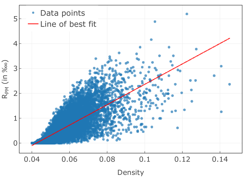
(b) BET-HILL for 0.1 bpnz (QF=75)

Figure 6: The scatter plot of $R_{PM}$ vs. the density of steganography modification, the corresponding Pearson correlation coefficients for the two cases are 0.95 and 0.70 respectively.

From Fig. 4, we also observe that for a given payload, the values of $R_{PM}$ will change a lot for different images. Taking HILL for 0.1 bpp for instance, the minimum of $R_{PM}$ is close to 0, while the maximum become close to 30, meaning the range of $R_{PM}$ is over 20 in this case. Furthermore, the range will increase with increasing payload or quality factor. In this section, we will analyze the factor which affects the values of $R_{PM}$.

Fig. 5 shows the steganography modifications and the post-modifications of two typical images using HILL for payload 0.1 bpp. From Fig. 5, we observe that for the first image, the steganography modifications seem uniformly dispersed throughout the whole image, while it is highly concentrated on a small part for the second one. After performing our method, the numbers of the post-modification are 1 and 523 separately. Thus we expect that there should be a positive correlation between the relative post-modification rate $R_{PM}$ and the density of steganography modification. To verify this, we define the density of steganography modification in the following way. We first compare the difference between cover $X$ and stego $Y$, and divide the difference (i.e. $Y\not=X$) into $5\times 5$ overlapping small blocks. And then we just consider those blocks which contain steganography modification, denoted as as $B_{i},i=1,2\ldots N$. For each block $B_{i}$, we calculate the proportion of steganography modification $|B_{i}|/25$, where $|B_{i}|$ denotes the number of steganography modification in block $B_{i}$, $0<|B_{i}|/25\leq 1$. Finally, we define the density of steganography modification for the stego image $Y$ as follows.

$$D_{Y}=\frac{1}{N}\sum_{n=1}^{N}\frac{|B_{i}|}{25}$$ (8)

Based on this definition, the densities of two images in Fig.5 are 0.05 and 0.27 respectively. We further calculate $R_{PM}$ and the density for 10,000 images in BOSSBase, and show the scatter plot for HILL (0.1 bpp) and BET-HILL (0.1 bpnz, QF=75) in Fig 6. For display purpose, we remove outlying data (less than 0.15% with larger values) in this figure. From Fig. 6, it is obvious that $R_{PM}$ increases with increasing density. In this case, the corresponding Pearson correlation coefficients are 0.95 and 0.70 respectively, meaning the linear relationships between the $R_{PM}$ and the density are relatively strong, which fits our expectation well. Similar results can be found for other steganographic methods and payloads.

IV-D Evaluation on Processing Time

TABLE XVII: Processing time (s) comparison with different methods in spatial domain.

	0.1	0.2	0.3	0.4	0.5
S-UNI	0.30	0.28	0.29	0.28	0.29
S-UNI-SPP	0.17	0.20	0.23	0.27	0.31
MIPOD	1.68	1.78	1.84	1.90	1.90
MIPOD-SPP	0.17	0.20	0.25	0.29	0.34
HILL	0.19	0.19	0.19	0.19	0.19
HILL-SPP	0.18	0.21	0.25	0.29	0.34
CMD-HILL Embed	0.32	0.33	0.32	0.32	0.32
CMD-HILL SPP	0.19	0.23	0.28	0.33	0.38

TABLE XVIII: Processing time (s) comparison with different methods in JPEG domain.

QF	Steganography	0.1	0.2	0.3	0.4	0.5
75	J-UNI	3.07	3.07	3.07	3.07	3.06
	J-UNI-SPP	0.47	0.48	0.49	0.50	0.50
	UERD	0.08	0.08	0.07	0.07	0.07
	UERD-SPP	0.47	0.48	0.49	0.49	0.50
	BET-HILL	0.68	0.69	0.69	0.69	0.69
	BET-HILL-SPP	0.47	0.48	0.48	0.49	0.50
95	J-UNI Embed	3.06	3.06	3.08	3.04	3.05
	J-UNI SPP	0.48	0.50	0.52	0.54	0.56
	UERD	0.08	0.07	0.07	0.07	0.07
	UERD SPP	0.48	0.50	0.51	0.53	0.55
	BET-HILL	0.69	0.74	0.71	0.71	0.71
	BET-HILL SPP	0.48	0.50	0.51	0.53	0.56

In this section, we will evaluate the processing time of the proposed method. To achieve convincing results, we report the average results on 100 images randomly selected from BOSSBase. For comparison, we also provide the processing time of the corresponding steganography method. The average results are shown in Table XVII and Table XVIII. From the two tables, we have two following observations:

• For a given steganography method, the processing time usually increases with increasing payload since more steganography modification should be dealt with. Taking HILL for instance, the time processing is 0.18s for 0.1 bpp, while it becomes 0.34s for 0.5 bpp.

• For the same reason, for a given JPEG steganography method and a payload, the processing time usually increases with increasing quality factor. Taking BET-HILL for 0.5 bpnz for instance, the processing time is 0.50s for QF=75, while it increases to 0.56s for QF=95.

Overall, the processing time of the proposed method is very short (less than 0.60s per image in all cases), which is comparable to or even much shorter than that of the current steganography method.

TABLE XIX: Detection accuracies improvements (%) for spatial steganography on three image databases (i.e. BOSSBase, BOWS2 and ALASKA).

Steganography	Database	SRM			maxSRMd2			Xu-Net			SRNet			Average
		0.1	0.3	0.5	0.1	0.3	0.5	0.1	0.3	0.5	0.1	0.3	0.5
S-UNI	BOSSBase	0.33	1.47	1.39	0.41	1.42	1.61	0.48	2.96	2.99	-	-	-	1.45
	BOWS2	0.23	2.33	1.97	1.66	2.73	2.11	1.00	4.66	2.98	-	-	-	2.19
	ALASKA	0.21	0.65	1.08	0.38	1.18	0.98	-0.14	2.48	3.48	0.72	0.60	0.57	1.02
MIPOD	BOSSBase	-0.12	2.33	2.68	1.41	2.77	3.01	1.08	4.31	5.20	-	-	-	2.52
	BOWS2	0.57	3.32	4.94	1.47	4.92	4.03	1.92	5.23	5.21	-	-	-	3.51
	ALASKA	0.25	1.34	1.86	0.64	1.82	2.17	1.32	4.47	4.61	0.55	0.81	1.16	1.75
HILL	BOSSBase	0.56	2.76	3.20	1.61	2.24	2.69	1.75	4.48	4.73	-	-	-	2.67
	BOWS2	1.52	4.75	5.04	2.76	4.54	4.22	2.66	5.92	5.67	-	-	-	4.12
	ALASKA	0.03	1.05	1.25	0.92	1.86	1.79	0.93	4.11	6.11	0.88	0.41	0.62	1.67
CMD-HILL	BOSSBase	0.54	0.91	1.68	0.39	0.93	0.96	0.42	2.01	3.14	-	-	-	1.22
	BOWS2	0.65	2.71	4.12	0.94	3.00	3.67	1.96	3.22	4.64	-	-	-	2.77
	ALASKA	0.46	0.46	1.11	0.30	1.18	1.58	-0.09	1.69	2.01	0.06	0.20	0.21	0.76

TABLE XX: Detection accuracies improvements (%) for JPEG steganography on three image databases (i.e. BOSSBase, BOWS2 and ALASKA).

QF	Steganography	Database	GFR			SCA-GFR			J-Xu-Net			SRNet			Average
			0.1	0.3	0.5	0.1	0.3	0.5	0.1	0.3	0.5	0.1	0.3	0.5
75	J-UNI	BOSSBase	-0.03	0.59	1.04	0.61	0.87	0.82	0.05	0.16	0.44	-	-	-	0.51
		BOWS2	-0.16	1.01	1.06	0.03	0.69	1.18	0.40	0.08	1.28	-	-	-	0.62
		ALASKA	0.06	0.38	1.44	0.28	1.18	1.20	0.06	0.92	1.58	-0.24	0.52	0.98	0.70
	UERD	BOSSBase	0.82	1.16	1.60	0.29	0.87	1.05	0.38	0.43	-0.12	-	-	-	0.72
		BOWS2	-0.11	1.07	1.43	0.63	0.96	1.08	1.25	2.35	0.52	-	-	-	1.02
		ALASKA	0.47	1.08	1.65	0.14	1.21	1.77	0.22	0.82	1.80	0.13	1.01	0.27	0.88
	BET-HILL	BOSSBase	0.44	1.92	1.68	1.11	2.26	1.99	1.35	1.61	1.47	-	-	-	1.54
		BOWS2	0.47	1.80	2.15	1.33	2.36	1.68	0.97	2.38	1.45	-	-	-	1.62
		ALASKA	-0.03	1.07	1.85	0.16	1.26	2.01	0.32	1.85	3.58	0.84	2.37	2.57	1.49
95	J-UNI	BOSSBase	0.10	0.60	1.65	0.07	1.23	1.73	0.18	1.09	-0.15	-	-	-	0.72
		BOWS2	0.03	0.95	2.66	0.08	1.27	2.60	-0.04	1.41	1.34	-	-	-	1.14
		ALASKA	0.06	0.36	1.47	0.04	0.23	1.52	0.03	0.47	1.76	0.00	0.36	1.23	0.63
	UERD	BOSSBase	0.07	1.83	3.09	0.27	1.72	2.79	0.08	0.09	0.67	-	-	-	1.18
		BOWS2	-0.11	1.50	3.85	0.27	2.20	2.96	0.01	1.93	-0.17	-	-	-	1.38
		ALASKA	0.14	0.96	2.26	0.02	1.58	2.58	-0.15	1.73	2.96	0.64	1.45	1.73	1.33
	BET-HILL	BOSSBase	0.18	1.08	2.73	0.72	1.97	2.77	0.57	1.27	1.93	-	-	-	1.47
		BOWS2	-0.04	1.08	4.13	0.23	2.09	3.05	0.20	2.32	1.64	-	-	-	1.63
		ALASKA	0.19	0.89	1.81	0.24	1.03	2.17	-0.03	0.42	1.91	0.02	1.68	3.21	1.13

IV-E Security Evaluation on Other Image Databases

In this section, we will evaluate the security performance on two other databases including 10,000 gray-scale images of size $512\times 512$ from BOWS2 [28] and 80,005 gray-scale images of size $256\times 256$ from ALASKA [29]. For BOWS2, the partition of image dataset and hyper-parameters are the same as previous ones used for the BOSSBase. For ALASKA, we randomly select 60,005 images for training while the other 20,000 for testing. In addition, the current best CNN-based steganalysis, i.e., SRNet [40], is used for security evaluation on ALASKA. For comparison, the detection accuracy improvements on the three image databases (i.e. BOSSBase, BOWS2 and ALASKA) are shown in Table XIX and Table XX. From the two tables, we obtain two following observations:

• Almost in all cases, the proposed method can effectively enhance the steganography security. In many cases, we can achieve over 3% and 2% for spatial and JPEG domains separately, which is a significant improvement on modern steganography. In a few cases, the security performance will drop slightly (less than 0.24%). On average, our method can enhance the steganography security for all cases (refer to the final column in two tables) .

• The improvement is different for the three image datasets. Compared to the results on BOSSBase and ALASKA, we can achieve greater improvements on BOWS2 in many cases, especially for steganography methods in spatial domain. In addition, the improvement would changes for different steganalytic methods. The improvement evaluated on the current best CNN-based steganalytic detector (i.e., SRNet) is relatively smaller than that on the there other detectors.

TABLE XXI: Detection accuracies improvements (%) of our previous method [26] and the proposed method for different steganography methods in spatial domain (0.4 bpp).

Steganography	S-UNI	MIPOD	HILL	CMD-HILL	Average
Method [26]	0.96	0.85	1.69	0.10	0.90
Proposed	1.37*	2.47*	3.30*	1.13*	2.07*

TABLE XXII: Detection accuracies improvements (%) of our previous method [26] and the proposed method for different steganography methods in JPEG domain (0.4 bpnz QF=95) .

Steganography	J-UNI	UERD	BET-HILL	Average
Method [26]	-0.19	-0.11	0.06	-0.08
Proposed	1.04*	2.54*	2.34*	1.97*

IV-F Comparison with Our Previous Method

In this section, we will compare the steganography security and the processing time with our previous work [26].

IV-F1 Comparison on Security Performance

For simplification, we evaluate spatial steganography methods for payload 0.4 bpp using SRM, and evaluate JPEG steganography methods for payload 0.4 bpnz with QF 95 using GFR both on BOSSBase. The experimental results are shown in Table XXI and Table XXII separately. From the two tables, we observe that in spatial domain, both methods can enhance steganography security. On average, the previous method and the proposed method achieve an improvement of about 1% and 2% separately. In JPEG domain, our previous method [26] does not work effectively, while the proposed method still achieves an average improvement of about 2%.

IV-F2 Comparison on Processing Time

The average processing time evaluated on 100 randomly selected images from BOSSBase are shown in Table XXIII and Table XXIV separately. From the two tables, we observe that the proposed method is significantly faster than the previous method. On average, the proposed method are able to achieve about 7 times acceleration in spatial domain, and about 5 times acceleration in JPEG domain.

The above results show that the proposed method is much more effective and faster than the previous one [26] .

TABLE XXIII: Processing time (s) for our previous method [26] and the proposed method for spatial steganography (0.4 bpp).

Steganography	S-UNI	MIPOD	HILL	CMD-HILL	Average
Method [26]	2.03	2.03	2.03	2.03	2.03
Proposed	0.27	0.29	0.29	0.33	0.30

TABLE XXIV: Processing time (s) for our previous method [26] and the proposed method for JPEG steganography (0.4 bpnz QF=95)

Steganography	J-UNI	UERD	BET-HILL	Average
Method [26]	2.79	2.78	2.78	2.78
Proposed	0.54	0.53	0.53	0.53

V Conclusion

In this paper, we propose a novel method to enhance the steganography security via stego post-processing. The main contributions of this paper are as follows.

• Unlike existing works which focus on embedding costs design (e.g., HILL and UNIWARD) or enhancement (e.g., CMD and BBC) according to some predetermined rules (such as complexity-first, spreading, clustering [41], and preserving the continuity of block boundary) during data embedding, the proposed method tries to directly modify embedding units of stego to reduce the residual distance when the embedding processing is completed with an existing steganography.

• The proposed method is universal, because it can be effectively applied in those steganographic methods using STCs for data hiding, including most modern image steganography methods both in spatial and JPEG domains. In addition, the number of modified embedding units is tiny with the proposed method.

• On average, the proposed method can enhance the steganography security in all cases. In many cases, we can even achieve over 3% and 2% for the modern steganographic methods in spatial and JPEG domain separately. Note that such an improvement is significant, especially for enhancing the advanced steganography, such as CMD-HILL and BET-HILL.

In our experiments, we try to reduce the Manhattan distance between cover residual and stego resudial via post-modification. Other steganalytic measures, such as the co-occurrence matrices of image residual in SRM and some deep learning based features will be considered in our future work. In addition, we will combine the technique of adversarial example to further improve the steganography security.

References

- [1] J. Fridrich and T. Filler, “Practical methods for minimizing embedding impact in steganography,” in Security, Steganography, and Watermarking of Multimedia Contents IX, vol. 6505, 2007, p. 650502.
- [2] T. Filler, J. Judas, and J. Fridrich, “Minimizing additive distortion in steganography using syndrome-trellis codes,” IEEE Transactions on Information Forensics and Security, vol. 6, no. 3, pp. 920–935, 2011.
- [3] T. Pevnỳ, T. Filler, and P. Bas, “Using high-dimensional image models to perform highly undetectable steganography,” in Springer International Workshop on Information Hiding, 2010, pp. 161–177.
- [4] V. Holub and J. Fridrich, “Designing steganographic distortion using directional filters,” in IEEE International Workshop on Information Forensics and Security, 2012, pp. 234–239.
- [5] V. Holub, J. Fridrich, and T. Denemark, “Universal distortion function for steganography in an arbitrary domain,” Springer EURASIP Journal on Information Security, vol. 2014, no. 1, p. 1, 2014.
- [6] B. Li, M. Wang, J. Huang, and X. Li, “A new cost function for spatial image steganography,” in IEEE International Conference on Image Processing, 2014, pp. 4206–4210.
- [7] V. Sedighi, R. Cogranne, and J. Fridrich, “Content-adaptive steganography by minimizing statistical detectability,” IEEE Transactions on Information Forensics and Security, vol. 11, no. 2, pp. 221–234, 2016.
- [8] B. Li, M. Wang, X. Li, S. Tan, and J. Huang, “A strategy of clustering modification directions in spatial image steganography,” IEEE Transactions on Information Forensics and Security, vol. 10, no. 9, pp. 1905–1917, 2015.
- [9] T. Denemark and J. Fridrich, “Improving steganographic security by synchronizing the selection channel,” in ACM Workshop on Information Hiding and Multimedia Security, 2015, pp. 5–14.
- [10] W. Zhang, Z. Zhang, L. Zhang, H. Li, and N. Yu, “Decomposing joint distortion for adaptive steganography,” IEEE Transactions on Circuits and Systems for Video Technology, vol. 27, no. 10, pp. 2274–2280, 2017.
- [11] L. Guo, J. Ni, and Y. Q. Shi, “Uniform embedding for efficient JPEG steganography,” IEEE transactions on Information Forensics and Security, vol. 9, no. 5, pp. 814–825, 2014.
- [12] L. Guo, J. Ni, W. Su, C. Tang, and Y.-Q. Shi, “Using statistical image model for JPEG steganography: uniform embedding revisited,” IEEE Transactions on Information Forensics and Security, vol. 10, no. 12, pp. 2669–2680, 2015.
- [13] X. Hu, J. Ni, and Y.-Q. Shi, “Efficient JPEG steganography using domain transformation of embedding entropy,” IEEE Signal Processing Letters, vol. 25, no. 6, pp. 773–777, 2018.
- [14] W. Li, W. Zhang, K. Chen, W. Zhou, and N. Yu, “Defining joint distortion for JPEG steganography,” in ACM Workshop on Information Hiding and Multimedia Security, 2018, pp. 5–16.
- [15] K. Chen, W. Zhang, H. Zhou, N. Yu, and G. Feng, “Defining cost functions for adaptive steganography at the microscale,” in IEEE International Workshop on Information Forensics and Security, 2016, pp. 1–6.
- [16] K. Chen, H. Zhou, W. Zhou, W. Zhang, and N. Yu, “Defining cost functions for adaptive JPEG steganography at the microscale,” IEEE Transactions on Information Forensics and Security, vol. 14, no. 4, pp. 1052–1066, 2018.
- [17] W. Zhou, W. Zhang, and N. Yu, “A new rule for cost reassignment in adaptive steganography,” IEEE Transactions on Information Forensics and Security, vol. 12, no. 11, pp. 2654–2667, 2017.
- [18] W. Zhou, W. Li, K. Chen, H. Zhou, W. Zhang, and N. Yu, “Controversial ’pixel’ prior rule for JPEG adaptive steganography,” IET Image Processing, vol. 13, no. 1, pp. 24–33, 2018.
- [19] I. Goodfellow, J. Pouget-Abadie, M. Mirza, B. Xu, D. Warde-Farley, S. Ozair, A. Courville, and Y. Bengio, “Generative adversarial nets,” in Advances in neural information processing systems, 2014, pp. 2672–2680.
- [20] C. Szegedy, W. Zaremba, I. Sutskever, J. Bruna, D. Erhan, I. Goodfellow, and R. Fergus, “Intriguing properties of neural networks,” arXiv preprint arXiv:1312.6199, 2013.
- [21] W. Tang, S. Tan, B. Li, and J. Huang, “Automatic steganographic distortion learning using a generative adversarial network,” IEEE Signal Processing Letters, vol. 24, no. 10, pp. 1547–1551, 2017.
- [22] J. Yang, D. Ruan, J. Huang, X. Kang, and Y.-Q. Shi, “An embedding cost learning framework using gan,” IEEE Transactions on Information Forensics and Security, 2019, To be appeared.
- [23] J. Yang, D. Ruan, X. Kang, and Y.-Q. Shi, “Towards automatic embedding cost learning for JPEG steganography,” in ACM Workshop on Information Hiding and Multimedia Security, 2019, pp. 37–46.
- [24] W. Tang, B. Li, S. Tan, M. Barni, and J. Huang, “Cnn-based adversarial embedding for image steganography,” IEEE Transactions on Information Forensics and Security, vol. 14, no. 8, pp. 2074–2087, 2019.
- [25] S. Bernard, T. Pevnỳ, P. Bas, and J. Klein, “Exploiting adversarial embeddings for better steganography,” in ACM Workshop on Information Hiding and Multimedia Security, 2019, pp. 216–221.
- [26] B. Chen, W. Luo, and P. Zheng, “Enhancing steganography via stego post-processing by reducing image residual difference,” in ACM Workshop on Information Hiding and Multimedia Security, 2019, pp. 63–68.
- [27] P. Bas, T. Filler, and T. Pevnỳ, “”break our steganographic system”: The ins and outs of organizing boss,” in Springer International Workshop on Information Hiding, 2011, pp. 59–70.
- [28] P. Bas and T. Furon, “Bows2,” http://bows2.ec-lille.fr, 2007.
- [29] R. Cogranne, Q. Giboulot, and P. Bas, “The alaska steganalysis challenge: A first step towards steganalysis ”into the wild”,” in ACM Workshop on Information Hiding and Multimedia Security, 2019, pp. 125–137.
- [30] N. Provos, “Defending against statistical steganalysis.” in Usenix security symposium, vol. 10, 2001, p. 323?336.
- [31] J. Fridrich and J. Kodovsky, “Rich models for steganalysis of digital images,” IEEE Transactions on Information Forensics and Security, vol. 7, no. 3, pp. 868–882, 2012.
- [32] X. Song, F. Liu, C. Yang, X. Luo, and Y. Zhang, “Steganalysis of adaptive JPEG steganography using 2d gabor filters,” in ACM Workshop on Information Hiding and Multimedia Security, 2015, pp. 15–23.
- [33] G. Xu, H.-Z. Wu, and Y.-Q. Shi, “Structural design of convolutional neural networks for steganalysis,” IEEE Signal Processing Letters, vol. 23, no. 5, pp. 708–712, 2016.
- [34] J. Ye, J. Ni, and Y. Yi, “Deep learning hierarchical representations for image steganalysis,” IEEE Transactions on Information Forensics and Security, vol. 12, no. 11, pp. 2545–2557, 2017.
- [35] G. Xu, “Deep convolutional neural network to detect j-uniward,” in ACM Workshop on Information Hiding and Multimedia Security, 2017, pp. 67–73.
- [36] A. D. Ker and R. Böhme, “Revisiting weighted stego-image steganalysis,” in Security, Forensics, Steganography, and Watermarking of Multimedia Contents X, vol. 6819, 2008, p. 681905.
- [37] T. Denemark, V. Sedighi, V. Holub, R. Cogranne, and J. Fridrich, “Selection-channel-aware rich model for steganalysis of digital images,” in IEEE International Workshop on Information Forensics and Security, 2014, pp. 48–53.
- [38] T. D. Denemark, M. Boroumand, and J. Fridrich, “Steganalysis features for content-adaptive JPEG steganography,” IEEE Transactions on Information Forensics and Security, vol. 11, no. 8, pp. 1736–1746, 2016.
- [39] J. Kodovsky, J. Fridrich, and V. Holub, “Ensemble classifiers for steganalysis of digital media,” IEEE Transactions on Information Forensics and Security, vol. 7, no. 2, pp. 432–444, 2012.
- [40] M. Boroumand, M. Chen, and J. Fridrich, “Deep residual network for steganalysis of digital images,” IEEE Transactions on Information Forensics and Security, vol. 14, no. 5, pp. 1181–1193, 2018.
- [41] B. Li, S. Tan, M. Wang, and J. Huang, “Investigation on cost assignment in spatial image steganography,” IEEE Transactions on Information Forensics and Security, vol. 9, no. 8, pp. 1264–1277, 2014.