Contributions of box diagrams and $\Delta(1940)$ resonance to $K^{0}\Sigma^{+}$ photoproduction

Abstract

We study first the box-diagram contribution to the $\gamma p\,\rightarrow\,K^{0}\Sigma^{+}$  process to understand the anomaly of the kaon photoproduction cross section from CBELSA/TAPS experiment at Electron Stretcher Accelerator (ELSA), where the imaginary part of the scattering amplitude from the box-diagrams is calculated by using Cutkosky’s rules in the on-shell approximation while the real part of the amplitude is derived by dispersion relation calculations. Together with the results of the K-MAID model, the contribution of the box-diagrams fails to provide the sudden drop of the differential cross-section between the $K^{*}\,\Lambda$ and $K^{*}\,\Sigma$ thresholds. In addition, we include the $\Delta(1940)$ resonance in the process to complete the description of the differential cross-section. Combining the contributions from the K-MAID model, the box-diagrams and the $\Delta(1940)$ resonance, we have obtained the theoretical differential cross-section the $\gamma p\,\rightarrow\,K^{0}\Sigma^{+}$  process, which is compatible with the CBELSA/TAPS experimental data.

I Introduction

The study of photoproduction processes is an effective tool to investigate the internal structures of the baryon excitations Hey and Kelly (1983); Glozman (1996); Anisovich et al. (2007); Klempt and Richard (2010); Aznauryan and Burkert (2012); Crede and Roberts (2013) as well as the hadronic interactions and its dynamical generated resonances and quasi-bound states Kaiser et al. (1997); Nacher et al. (1999); Soyeur and Lutz (2005); Liu et al. (2008); Wang et al. (2015); Chen et al. (2016); Guo et al. (2018); Liu et al. (2019). One of the theoretical milestone was accomplished by Kroll and Rundermann Kroll and Ruderman (1954). The Kroll-Runderman theorem provides model-independent predictions of cross sections for pion photoproduction, i.e., $\gamma N\rightarrow\pi N$, in the threshold region by applying the gauge and Lorentz invariance. Later, the general formalism of scattering amplitudes is constructed by Chew, Goldberger, Low and Nambu Chew et al. (1957), known as CGLN amplitudes for single-pion photoproduction from the nucleon, which provides a systematic and convenient framework of theoretical calculations to compare with the experimental observables at the low-energies regime. Numerous research works on both theoretical and phenomenological approaches have been done so far, for example, phenomenological Lagrangian Dalitz et al. (1967); Thom (1966); Berends et al. (1967); Walker (1969); Adelseck et al. (1985); Workman (1989); Adelseck and Saghai (1990); Drechsel and Tiator (1992); Steininger and Meissner (1997); Guidal et al. (1997), coupled-channel dynamics Kaiser et al. (1997); Borasoy et al. (2007); Julia-Diaz et al. (2008); Huang et al. (2012); Ronchen et al. (2013) and quark models Copley et al. (1969); Li (1995); Li et al. (1997); Zhao et al. (2002); Zhong and Zhao (2011). One of the reasonably successful models of the meson photoproduction is the so-called MAID which is developed by a research group at Mainz University Knochlein et al. (1995); Drechsel et al. (1999); Kamalov et al. (2001); Chiang et al. (2002, 2003); Drechsel et al. (2007); Hilt et al. (2013) (see Tiator et al. (2011); Tiator (2018) for recent reviews) based on chiral effective Lagrangian in the Born approximation with observed resonant channels. The model has been extended to the strangeness sector of the meson photoproduction (called K-MAID Lee et al. (2001)), and the theoretical predictions of the K-MAID are well consistent with the experimental data at the center of mass energy below 2 GeV Mart and Bennhold (2000); Bennhold et al. (2000, 1999).

The CBELSA/TAPS experiment at the Electron Stretcher Accelerator (ELSA) of Bonn University has investigated the excitation spectrum of the nucleon in the $\gamma p\rightarrow K^{0}\Sigma^{+}$ photoproduction reaction at low-energy region, i.e., the center of mass energy from 1.70 to 2.25 GeV Ewald et al. (2012). The differential cross section raises with increasing the energy up to the $K^{*}\Lambda$ threshold, and then drops rapidly in the energy region of 2.0074 $-$ 2.0855 GeV, and finally turns to a rather flat distribution at high energies. This result reveals the anomaly of the different cross-section at forward angle in the $K^{*}\Lambda$ and $K^{*}\Sigma$ regime. The K-MAID result is expected to describe the $\gamma p\rightarrow K^{0}\Sigma^{+}$ data. According to the differential cross-section in Ref. Ewald et al. (2012), however, one finds that the theoretical result of the K-MAID model is in line with the data at the very low energy region only. The modification of the parameters of the K-MAID (modified K-MAID) is also taken into account and the result of the modified K-MAID is compatible with the differential cross-section data at beyond the $K^{*}\Sigma$ threshold region. The discrepancy between the experimental data and the theoretical results from both the K-MAID and modified K-MAID models indicates that it is necessary to further improve the K-MAID model by adding new physics or more mechanism to the $\gamma p\rightarrow K^{0}\Sigma^{+}$ photoproduction reaction. The solution of this discrepancy has been speculated in Ewald et al. (2012) that the contributions of the dynamically generated quasi-bound states for $K^{*}\Lambda$ and $K^{*}\Sigma$ should play crucial role to the differential cross-section in the $K^{*}\Lambda$ and $K^{*}\Sigma$ thresholds. To include this physical mechanism to the reaction, one may calculate the coupled-channel effects of the vector-meson and baryon interactions or box-diagram in the on-shell approximation of the intermediated states. In addition, the similar results of the $K^{0}\Sigma^{+}$ photoproduction have been found previously in Crystal Barrel experiment Castelijns et al. (2008).

After the speculation of the anomaly of $K^{0}\Sigma^{+}$ photoproduction was proposed in Ref. Ewald et al. (2012), the cross-section of the $\gamma p\rightarrow K^{0}\Sigma^{+}$ reaction is investigated Ramos and Oset (2013), by applying a chiral unitary coupled-channel approach with the effective chiral vector-meson and baryon interactions from hidden gauge formalism. The results in Ref. Ramos and Oset (2013) exhibit the sudden drop of the cross-section in the region of the $K^{*}\Lambda$ and $K^{*}\Sigma$ thresholds and it is compatible with the experimental data.

In this work, we will carry out detailed calculations for the one-loop box-diagrams of the $\gamma p\rightarrow K^{0}\Sigma^{+}$ reaction in chiral effective Lagrangians by using the Cutkosky rules or the on-shell approximation of the intermediated states. In addition, we also include relevant Born diagrams with modified parameters of the K-MAID as well as contributions from $N^{*}$ and $\Delta^{*}$ resonances. We expect to shed some light on the understanding of the anomaly of the different cross-section from the CBELSA/TAPS experiment and the work would be of some value for the understanding of hadronic structures and interactions in the $K^{0}\Sigma$ photoproduction process. We outline this work as follows: the ingredients of the box-diagrams and related formalisms are presented in the section II. The numerical results of the box-diagrams in on-shell approximation, modified K-MAID and additional baryon resonance are shown in the section III. In the last section, we will give the discussions and conclusions of this work.

II Formalism

In this section, we present the formalisms for studying the differential cross-section in the $\gamma p\,\rightarrow\,K^{0}\Sigma^{+}$ process. We divide the ingredients of our formalisms into three parts as the box-diagrams, modified K-MAID and baryon resonance. The details of these ingredients are given in the following subsections.

II.1 The box-diagram calculations in the on-shell scheme

II.1.1 Effective Lagrangian for kaon-photoproduction process

The relevant Feynman box-diagrams for the $\gamma p\,\rightarrow\,K^{0}\Sigma^{+}$ process are depicted in Fig. 1. The chiral effective Lagrangian for the $\gamma\,K^{*}\,K$ coupling is given by Hyodo et al. (2004); Oh et al. (2004)

$$\mathscr{L}_{\gamma\,\bar{K}^{*}\,K} = g_{\gamma\,\bar{K}^{*}\,K}\,\epsilon_{\mu\nu\alpha\beta}\,\partial^{\mu}\,A^{\nu}\,\partial^{\alpha}\,\bar{K}^{*,\,\beta}\,K+{\rm h.c.}\,,$$ (1)

and the chiral effective Lagrangian for the $\pi\,K^{*}\,K$ coupling reads Hyodo et al. (2004); Palomar and Oset (2003)

$$\mathscr{L}_{\pi\,K^{*}\,\bar{K}} = -\,i\,g_{\pi\,K^{*}\,\bar{K}}\Big{\{}\,\bar{K}\,\vec{\tau}\cdot\,\partial_{\mu}\,\vec{\pi}\,K^{*\,\mu}$$ (2)

$$\qquad\qquad\quad\;-\,(\partial_{\mu}\,\bar{K})\,\vec{\tau}\cdot\,\vec{\pi}\,K^{*\,\mu}\,\Big{\}}+{\rm h.c.}\,.$$

For the meson-baryon interactions, we employ the axial-coupling vertices which are written in terms of the isospin basis Chiang et al. (2004)

$$\mathscr{L}_{K\,N\,\Lambda} = -\,\frac{g_{K\,N\,\Lambda}}{M_{\pi}}\,\bar{\Lambda}\,\gamma^{\mu}\,\gamma_{5}\,(\partial_{\mu}\,\bar{K})\,N+{\rm h.c.}\,,$$

$$\mathscr{L}_{K\,N\,\Sigma} = -\,\frac{g_{K\,N\,\Sigma}}{M_{\pi}}\,\,\vec{\bar{\Sigma}}\,\cdot(\,\gamma^{\mu}\,\gamma_{5}\,\partial_{\mu}\,\bar{K}\,\vec{\tau}\,N)+{\rm h.c.}\,,$$

$$\mathscr{L}_{\pi\,\Lambda\,\Sigma} = -\,\frac{g_{\pi\,\Lambda\,\Sigma}}{M_{\pi}}\,\,(\vec{\bar{\Sigma}}\,\gamma^{\mu}\,\gamma_{5}\,\Lambda)\,\cdot\,\partial_{\mu}\,\vec{\pi}+{\rm h.c.}\,,$$

$$\mathscr{L}_{\pi\,\Sigma\,\Sigma} = i\,\frac{g_{\pi\,\Sigma\,\Sigma}}{M_{\pi}}\,\big{(}\vec{\bar{\Sigma}}\,\gamma^{\mu}\,\gamma_{5}\,\times\,\vec{\Sigma}\big{)}\,\cdot\,\partial_{\mu}\,\vec{\pi}\,,$$ (3)

where the phase convention of mesons and baryons in the isospin basis is defined by

$$N = \left(\begin{array}[]{c}p\\ n\end{array}\right)\,,~{}~{}~{}~{}K=\left(\begin{array}[]{c}K^{+}\\ K^{0}\end{array}\right)\,,~{}~{}~{}~{}K^{*}=\left(\begin{array}[]{c}K^{+\,*}\\ K^{0\,*}\end{array}\right)\,,$$ (10)

$$\vec{\pi} = \left\{{\textstyle{\frac{1}{\sqrt{2}}}}\,(\pi^{+}+\pi^{-})\,,\;{\textstyle{\frac{i}{\sqrt{2}}}}\,(\pi^{+}-\pi^{-})\,,\;\pi^{0}\right\}\,,$$

$$\vec{\Sigma} = \left\{{\textstyle{\frac{1}{\sqrt{2}}}}\,(\Sigma^{+}+\Sigma^{-})\,,\;{\textstyle{\frac{i}{\sqrt{2}}}}\,(\Sigma^{+}-\Sigma^{-})\,,\;\Sigma^{0}\right\}$$

The isospin generators $\vec{\tau}$  are usual Pauli matrices,

$$\vec{\tau}=\left\{\tau_{1}\,,\;\tau_{2}\,,\;\tau_{3}\right\}=\left\{\left(\begin{array}[]{cc}0&1\\ 1&0\end{array}\right)\,,\;\left(\begin{array}[]{cc}0&-i\\ i&0\end{array}\right)\,,\;\left(\begin{array}[]{cc}1&0\\ 0&-1\end{array}\right)\right\}.$$

II.1.2 Imaginary part of the scattering amplitudes in the on-shell scheme

We calculate here the scattering amplitudes of the box-diagrams for $K^{0}\Sigma$-photoproduction in the on-shell approximation.

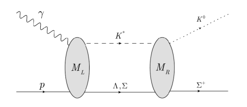
Figure 1: Box-diagrams: Vector kaons and hyperons generated as the intermediated particles, and then inelastically re-scattered to the $K^{0}\Sigma^{+}$ final state.

First of all, we assign the four-momenta for each particles as

$$\gamma=\gamma(k)\,,\quad p=p(p)\,,\quad K^{0}=K^{0}(q)\,,\quad$$

$$\Sigma^{+}=\Sigma(\bar{p})\,,\quad K^{*}=K^{*}(l)\,.$$ (11)

In this work, we apply the Cutkosky rules to our box-diagram calculations. The formalism is to calculate the imaginary part of scattering amplitudes based on the optical theorem of the Feynman diagrams (for more detailed discussion see Ref. Peskin and Schroeder (1995)). The physical meaning of the scheme is that there are re-scattering effects between mesons and baryons in the intermediate states. The imaginary part of scattering amplitudes of the box-diagrams takes the generic form

$${\rm Im}\,\mathcal{M}_{\rm box}=-\frac{\widetilde{l}}{32\,\pi^{2}\,\sqrt{s}}\int d\,\Omega\,\sum_{K^{*},Y}\,M_{L}\big{(}\gamma p\,\rightarrow\,K^{*}Y\big{)}\,M_{R}^{\dagger}\big{(}K^{0}\Sigma^{+}\rightarrow K^{*}Y\,\big{)}$$ (12)

where the summation of overall intermediated particles spin is implied, $Y=\Lambda,\,\Sigma$, and $\widetilde{l}$ is the 3-momentum magnitude in the c.m. frame of intermediate $K^{*}$ particle, reading as

$$\widetilde{l}=\sqrt{\frac{\big{[}s-(m_{K^{*}}-m_{Y})^{2}\big{]}\big{[}s-(m_{K^{*}}+m_{Y})^{2}\big{]}}{4\,s}}\,.$$ (13)

We obtain, from the above effective Lagrangians, the amplitudes $M_{L}$ and $M_{R}$  (see Fig. 2 for corresponding Feynman diagrams of $M_{L}$  and $M_{R}$),

$$M_{L}^{(1)}\big{(}\gamma p\,\rightarrow\,K^{*,+}\Lambda\big{)} = -\,g_{\gamma\,\bar{K}^{*}\,K}^{(c)}\,\frac{g_{K\,N\,\Lambda}}{m_{\pi}}\,\epsilon_{\mu\nu\alpha\beta}\,k^{\mu}\,\epsilon_{(\gamma)}^{\nu}\,l^{\alpha}\,\epsilon_{(K^{*})}^{*\beta}\,\frac{\bar{u}_{\Lambda}\,(k\!\!\!/-l\!\!\!/)\,\gamma_{5}\,u_{p}}{(k-l)^{2}-m_{\bar{K}}^{2}}\,F_{K}^{2}(k-l)\,,$$ (14)

$$M_{L}^{(2)}\big{(}\gamma p\,\rightarrow\,K^{*,0}\Sigma^{+}\big{)} = -\sqrt{2}\,g_{\gamma\,\bar{K}^{*}\,K}^{(0)}\,\frac{g_{K\,N\,\Sigma}}{m_{\pi}}\,\epsilon_{\mu\nu\alpha\beta}\,k^{\mu}\,\epsilon_{(\gamma)}^{\nu}\,l^{\alpha}\,\epsilon_{(K^{*})}^{*\beta}\,\frac{\bar{u}_{\Sigma}\,(k\!\!\!/-l\!\!\!/)\,\gamma_{5}\,u_{p}}{(k-l)^{2}-m_{\bar{K}}^{2}}\,F_{K}^{2}(k-l)\,,$$ (15)

$$M_{L}^{(3)}\big{(}\gamma p\,\rightarrow\,K^{*,+}\Sigma^{0}\big{)} = -\,g_{\gamma\,\bar{K}^{*}\,K}^{(c)}\,\frac{g_{K\,N\,\Sigma}}{m_{\pi}}\,\epsilon_{\mu\nu\alpha\beta}\,k^{\mu}\,\epsilon_{(\gamma)}^{\nu}\,l^{\alpha}\,\epsilon_{(K^{*})}^{*\beta}\,\frac{\bar{u}_{\Sigma}\,(k\!\!\!/-l\!\!\!/)\,\gamma_{5}\,u_{p}}{(k-l)^{2}-m_{\bar{K}}^{2}}\,F_{K}^{2}(k-l)\,,$$ (16)

$$M_{R}^{(1),\dagger}\big{(}K^{0}\Sigma^{+}\rightarrow\,K^{*,+}\Lambda\,\big{)} = 2\,\sqrt{2}\,g_{\pi\,K^{*}\,\bar{K}}\,\frac{g_{\pi\,\Lambda\,\Sigma}}{m_{\pi}}\,q_{\mu}\,\epsilon_{(K^{*})}^{\mu}\,\frac{\bar{u}_{\Sigma}\,(l\!\!\!/-q\!\!\!/)\,\gamma_{5}\,u_{\Lambda}}{(l-q)^{2}-m_{\pi}^{2}}\,F_{\pi}^{2}(l-q)\,,$$ (17)

$$M_{R}^{(2),\dagger}\big{(}K^{0}\Sigma^{+}\rightarrow\,K^{*,0}\Sigma^{+}\big{)} = -\,2\,g_{\pi\,K^{*}\,\bar{K}}\,\frac{g_{\pi\,\Sigma\,\Sigma}}{m_{\pi}}\,q_{\mu}\,\epsilon_{(K^{*})}^{\mu}\,\frac{\bar{u}_{\Sigma}\,(l\!\!\!/-q\!\!\!/)\,\gamma_{5}\,u_{\Sigma}}{(l-q)^{2}-m_{\pi}^{2}}\,F_{\pi}^{2}(l-q)\,,$$ (18)

$$M_{R}^{(3),\dagger}\big{(}K^{0}\Sigma^{+}\rightarrow\,K^{*,+}\Sigma^{0}\big{)} = 2\,g_{\pi\,K^{*}\,\bar{K}}\,\frac{g_{\pi\,\Sigma\,\Sigma}}{m_{\pi}}\,q_{\mu}\,\epsilon_{(K^{*})}^{\mu}\,\frac{\bar{u}_{\Sigma}\,(l\!\!\!/-q\!\!\!/)\,\gamma_{5}\,u_{\Sigma}}{(l-q)^{2}-m_{\pi}^{2}}\,F_{\pi}^{2}(l-q)\,,$$ (19)

where $u_{p,\Sigma,\Lambda}$ stand for the spinors of the proton, $\Sigma$ and $\Lambda$ baryons respectively, and $\epsilon_{(\gamma,K^{*})}^{\mu}$ are the polarization vectors of the photon and vector $K^{*}$ meson respectively. $F_{X}(q)$ are form-factors introduced to regularize the high momentum behavior of the meson-baryon couplings, taking the form,

$$F_{X}(q)=\frac{\Lambda_{X}^{2}-m_{X}^{2}}{\Lambda_{X}^{2}-q^{2}}\,,$$ (20)

where $X=K\,,~{}\pi$ . Here we take $\Lambda_{K}=900$ MeV and $\Lambda_{\pi}=450$ MeV. Note that the identity $l^{\mu}\,\epsilon_{\mu}^{*}(l\,,m_{K^{*}})=0$  is applied to above equations.

As the data analysis of the experimental results and the speculation from Ref. Ewald et al. (2012) indicate that the $t$-channel is dominant, we consider the $t$-channel amplitudes for the on-shell intermediate states only. Then the imaginary part of scattering amplitude can be written in the following form,

$${\rm Im}\,\mathcal{M}_{\rm box}={\rm Im}\,\mathcal{M}_{\rm box}^{(1)}+{\rm Im}\,\mathcal{M}_{\rm box}^{(2)}+{\rm Im}\,\mathcal{M}_{\rm box}^{(3)}\,.$$ (21)

The ${\rm Im}\,\mathcal{M}_{\rm box}^{(1)}$ amplitude reads,

$${\rm Im}\,\mathcal{M}_{\rm box}^{(1)} = -\frac{\widetilde{l}}{32\,\pi^{2}\,\sqrt{s}}\int d\,\Omega\,\sum_{K^{*,+},\Lambda}\,M_{L}^{(1)}\big{(}\gamma p\rightarrow K^{*,+}\Lambda\big{)}\,M_{R}^{(1)\;\dagger}\big{(}K^{0}\Sigma^{+}\rightarrow K^{*,+}\Lambda\big{)}$$

$$= \frac{\widetilde{l}}{64\,\pi^{2}\,\sqrt{s}}\,G_{1}\int d\,\Omega\;\frac{F_{K}^{2}(k-l)}{(k-l)^{2}-m_{\bar{K}}^{2}}\,\frac{F_{\pi}^{2}(l-q)}{(l-q)^{2}-m_{\pi}^{2}}$$

$$\times\,\bar{u}_{\Sigma}\,\big{(}k\!\!\!/\,\epsilon\!\!\!/\,q\!\!\!/\,l\!\!\!/-l\!\!\!/\,k\!\!\!/\,\epsilon\!\!\!/\,q\!\!\!/-k\cdot q\,l\!\!\!/\,\epsilon\!\!\!/+k\cdot l\,\epsilon\!\!\!/\,l\!\!\!/-q\cdot\epsilon\,k\!\!\!/\,l\!\!\!/+q\cdot\epsilon\,l\!\!\!/\,k\!\!\!/\big{)}\,\gamma_{5}\,(l\!\!\!/-q\!\!\!/)\,\gamma_{5}\,(p\!\!\!/+k\!\!\!/-l\!\!\!/+m_{\Lambda})\,(k\!\!\!/-l\!\!\!/)\,\gamma_{5}\,u_{p}\,,$$

where  $l^{2}=m_{K^{*}}^{2}$,  $k^{2}=0$,  and  $G_{1}=-\,2\,\sqrt{2}\,g_{\gamma\,\bar{K}^{*}\,K}^{(c)}\,g_{\pi\,K^{*}\,\bar{K}}\,\frac{g_{K\,N\,\Lambda}}{m_{\pi}}\,\frac{g_{\pi\,\Lambda\,\Sigma}}{m_{\pi}}\,$, and the scalar dot production of the four-vector is used by the notation $A\cdot B=A_{\mu}\,B^{\mu}=g_{\mu\nu}A^{\mu}\,B^{\nu}=g^{\mu\nu}A_{\mu}\,B_{\nu}$ . With the same manner, one obtains the imaginary part of scattering amplitudes, ${\rm Im}\,\mathcal{M}_{\rm box}^{(2)}$  and ${\rm Im}\,\mathcal{M}_{\rm box}^{(3)}$. They are given by

$${\rm Im}\,\mathcal{M}_{\rm box}^{(2)} = -\frac{\widetilde{l}}{32\,\pi^{2}\,\sqrt{s}}\int d\,\Omega\,\sum_{K^{*,0},\Sigma^{+}}\,M_{L}^{(2)}\big{(}\gamma p\,\rightarrow\,K^{*,0}\Sigma^{+}\big{)}\,M_{R}^{(2)\;\dagger}\big{(}K^{0}\Sigma^{+}\,\rightarrow\,K^{*,0}\Sigma^{+}\big{)}$$

$$= \frac{\widetilde{l}}{64\,\pi^{2}\,\sqrt{s}}\,G_{2}\int d\,\Omega\;\frac{F_{K}^{2}(k-l)}{(k-l)^{2}-m_{\bar{K}}^{2}}\,\frac{F_{\pi}^{2}(l-q)}{(l-q)^{2}-m_{\pi}^{2}}$$

$$\times\,\bar{u}_{\Sigma}\,\big{(}k\!\!\!/\,\epsilon\!\!\!/\,q\!\!\!/\,l\!\!\!/-l\!\!\!/\,k\!\!\!/\,\epsilon\!\!\!/\,q\!\!\!/-k\cdot q\,l\!\!\!/\,\epsilon\!\!\!/+k\cdot l\,\epsilon\!\!\!/\,l\!\!\!/-q\cdot\epsilon\,k\!\!\!/\,l\!\!\!/+q\cdot\epsilon\,l\!\!\!/\,k\!\!\!/\big{)}\,\gamma_{5}\,(l\!\!\!/-q\!\!\!/)\,\gamma_{5}\,(p\!\!\!/+k\!\!\!/-l\!\!\!/+m_{\Sigma})\,(k\!\!\!/-l\!\!\!/)\,\gamma_{5}\,u_{p}\,,$$

where  $G_{2}=2\,\sqrt{2}\,g_{\gamma\,\bar{K}^{*}\,K}^{(0)}\,g_{\pi\,K^{*}\,\bar{K}}\,\frac{g_{K\,N\,\Sigma}}{m_{\pi}}\,\frac{g_{\pi\,\Sigma\,\Sigma}}{m_{\pi}}\,$, and

$${\rm Im}\,\mathcal{M}_{\rm box}^{(3)} = -\frac{\widetilde{l}}{32\,\pi^{2}\,\sqrt{s}}\int d\,\Omega\,\sum_{K^{*,+},\Sigma^{0}}\,M_{L}^{(3)}\big{(}\gamma p\,\rightarrow\,K^{*,+}\Sigma^{0}\big{)}\,M_{R}^{(3)\;\dagger}\big{(}K^{0}\Sigma^{+}\,\rightarrow\,K^{*,+}\Sigma^{0}\big{)}$$

$$= \frac{\widetilde{l}}{64\,\pi^{2}\,\sqrt{s}}\,G_{3}\int d\,\Omega\;\frac{F_{K}^{2}(k-l)}{(k-l)^{2}-m_{\bar{K}}^{2}}\,\frac{F_{\pi}^{2}(l-q)}{(l-q)^{2}-m_{\pi}^{2}}$$

$$\times\,\bar{u}_{\Sigma}\,\big{(}k\!\!\!/\,\epsilon\!\!\!/\,q\!\!\!/\,l\!\!\!/-l\!\!\!/\,k\!\!\!/\,\epsilon\!\!\!/\,q\!\!\!/-k\cdot q\,l\!\!\!/\,\epsilon\!\!\!/+k\cdot l\,\epsilon\!\!\!/\,l\!\!\!/-q\cdot\epsilon\,k\!\!\!/\,l\!\!\!/+q\cdot\epsilon\,l\!\!\!/\,k\!\!\!/\big{)}\,\gamma_{5}\,(l\!\!\!/-q\!\!\!/)\,\gamma_{5}\,(p\!\!\!/+k\!\!\!/-l\!\!\!/+m_{\Sigma})\,(k\!\!\!/-l\!\!\!/)\,\gamma_{5}\,u_{p}\,,$$

where  $G_{3}=-\,2\,g_{\gamma\,\bar{K}^{*}\,K}^{(c)}\,g_{\pi\,K^{*}\,\bar{K}}\,\frac{g_{K\,N\,\Sigma}}{m_{\pi}}\,\frac{g_{\pi\,\Sigma\,\Sigma}}{m_{\pi}}\,$.

$\begin{array}[]{c}\includegraphics[width=312.9803pt,clip={true}]{mlr-2.pdf}\end{array}$

Figure 2: Feynman diagrams with all possible $K^{*}Y$ intermediate states in $t$-channel: (a) for $M_{L}^{(1,2,3)}\big{(}\gamma p\,\rightarrow\,K^{*}Y\big{)}$ and (b) for $M_{R}^{(1,2,3)}\big{(}K^{*}Y\rightarrow K^{0}\Sigma^{+}\big{)}$.

It is convenient to write the scattering amplitudes in terms of the CGLN amplitudes which have been widely employed to study the photoproduction processes Chew et al. (1957). The transition amplitudes in Eqs. (II.1.2,II.1.2,II.1.2) can be expressed in terms of the CGLN amplitudes,

$${\rm Im}\,\mathcal{M}_{\rm box}^{(i)}=\int_{-1}^{1}d(\cos\theta_{\rm in})\int_{0}^{2\pi}d\phi_{\rm in}$$

$$\qquad\times\,\Big{(}\mathcal{F}_{1}^{{\rm box}\,(i)}\vec{\sigma}\cdot\vec{\varepsilon}+\mathcal{F}_{2}^{{\rm box}\,(i)}i\,(\vec{\sigma}\cdot\hat{q}\,)\,(\vec{\varepsilon}\times\hat{k}\,)\cdot\,\vec{\sigma}$$

$$\qquad+\,\mathcal{F}_{3}^{{\rm box}\,(i)}(\vec{\sigma}\cdot\hat{k}\,)\,(\hat{q}\cdot\vec{\varepsilon}\,)+\mathcal{F}_{4}^{{\rm box}\,(i)}(\vec{\sigma}\cdot\hat{q}\,)\,(\hat{q}\cdot\vec{\varepsilon}\,)\Big{)}\,,$$ (25)

where index $i=1,2,3$ . The detailed derivation of the CGLN amplitudes of the box-diagrams is shown in the appendix, and the generic form of the CGLN amplitudes ($\mathcal{F}_{i}$) is given in Eq. (57). In the above equation, we have defined the kinematic variables in the c.m. frame. The (real) photon polarization has the component as  $\epsilon^{\mu}=\big{(}\,0\,,~{}\vec{\varepsilon}\;\big{)}$, and the components of the 3-momenta $\vec{k}\,,~{}\vec{l}$ and $\vec{q}$  are given by

$$\vec{k} = \widetilde{k}\,\big{(}\,0\,,~{}0\,,~{}1\,\big{)}\,,$$

$$\vec{l} = \widetilde{l}\,\big{(}\,\sin\theta_{\rm in}\,\cos\phi_{\rm in}\,,~{}\sin\theta_{\rm in}\,\sin\phi_{\rm in}\,,~{}\cos\theta_{\rm in}\,\big{)}\,,$$

$$\vec{q} = \widetilde{q}\,\big{(}\,\sin\theta\,,~{}0\,,~{}\cos\theta\,\big{)}\,,$$ (26)

here we used notation $|\vec{k}\;|=\widetilde{k}$ , $|\vec{l}\;|=\widetilde{l}$  and $|\vec{q}\;|=\widetilde{q}$  and all kinematic variables are in c.m. frame i.e. $\vec{k}=-\vec{p}$  and $\vec{q}=-\vec{\bar{p}}$ . In addition, the three-momenta, $\widetilde{k}$ , and $\widetilde{q}$  are written by

$$\widetilde{k} = \widetilde{p}=\frac{\sqrt{\big{[}s-m_{p}^{2}\big{]}\big{[}s-m_{p}^{2}\big{]}}}{2\sqrt{s}}\,,$$

$$\widetilde{q} = \widetilde{\bar{p}}=\frac{\sqrt{\big{[}s-(m_{\Sigma}-m_{K})^{2}\big{]}\big{[}s-(m_{\Sigma}+m_{K})^{2}\big{]}}}{2\sqrt{s}}\,.$$ (27)

In this work, the input parameters of the on-shell box-diagram calculation are taken from literatures, $g_{\pi K^{*}\bar{K}}=-\,3.26$ Usov and Scholten (2005) , $g_{\gamma K^{*}\bar{K}}^{(c)}=0.254~{}{\rm GeV}^{-1}$ Oh et al. (2004) , $g_{\gamma K^{*}\bar{K}}^{(0)}=0.388~{}{\rm GeV}^{-1}$ Oh et al. (2004) , $g_{KN\Lambda}=-\,0.95$ Chiang et al. (2004) , $g_{KN\Sigma}=0.27$ Chiang et al. (2004) , $g_{\pi\Lambda\Sigma}=0.71$ Chiang et al. (2004) , $g_{\pi\Sigma\Sigma}=0.74$Chiang et al. (2004) , $\Lambda_{K}=900$ MeV , $\Lambda_{\pi}=450$ MeV . The imaginary part of the box-diagram amplitudes will be calculated numerically and also employed to obtain the real part by using the dispersion relation in the next subsection.

II.1.3 The real part of the box diagram amplitudes

The intermediate states would contribute the dispersive (real) part of the box-diagram (loop) amplitudes beyond the $K^{*}\Lambda$ and $K^{*}\Sigma$ thresholds. The real part can be determined via the dispersion relation Guo et al. (2012),

$${\rm Re}\,\mathcal{M}_{\rm box}=\frac{1}{2\,\pi\,i}\,\mathcal{P}\left(\int_{M_{K^{*}\Lambda}^{2}}^{M_{K^{*}\Sigma}^{2}}\,\frac{{\rm Im}\,\mathcal{M}_{\rm box}(s^{\prime})}{s-s^{\prime}}\,d\,s^{\prime}+\int_{M_{K^{*}\Sigma}^{2}}^{\infty}\,\frac{{\rm Im}\,\mathcal{M}_{\rm box}(s^{\prime})}{s-s^{\prime}}\,d\,s^{\prime}\right),$$ (28)

where $\mathcal{P}$ stands for the principal value of the complex integration, and $M_{K^{*}\Lambda}$ and $M_{K^{*}\Sigma}$ are the thresholds of $K^{*}\Lambda$ and $K^{*}\Sigma$ masses respectively. The real part amplitudes are calculated numerically and we will show the results in the next section.

II.2 Modified K-MAID

In this work, we will use the K-MAID model as the first-order approximation to the $K^{0}\Sigma^{+}$ photoproduction (see Tiator (2018) for the latest status report). The K-MAID contains all possible Born amplitudes (tree-level) with $S$, $P$ and $D$ wave excitation states $N^{*}$ up to 1910 MeV. It has been demonstrated in Ref. Ewald et al. (2012) that the K-MAID can not satisfactorily describe the data. However, the K-MAID is still a good model and useful for studying the $\gamma p\rightarrow K^{0}\Sigma^{+}$ reaction below 1900 MeV by adjusting the model parameters. Moreover, the K-MAID model provides the CGLN amplitudes which can be incorporated to our box-diagram results directly. We extract the numerical value of CGLN amplitudes from the website www.kph.uni-mainz.de/MAID/kaon/ with modified parameters in the K-MAID model,

$$G1_{\rm S_{31}}(1900)=0.8\,,\qquad G1_{\rm P_{31}}(1910)=0.6\,,$$

$$G2_{\rm S_{31}}(1900)=0.8\,,\qquad G2_{\rm P_{31}}(1910)=0.6\,.$$ (29)

The result of the modified K-MAID with respect to the data is depicted as dashed line in Fig. 3 (upper panel). With the proper modification of the K-MAID parameters in Eq. (29), the result is compatible with the data up to c.m. frame energy around 1920 MeV. However, the modified K-MAID still mismatches the experimental results beyond 1920 MeV. This requires additional mechanism such as box-diagrams and baryon resonances to understand the data.

II.3 $\Delta(1940)$ resonance

To improve the K-MAID model results of the differential cross section below the $K^{*}\Lambda$ threshold around 1960-1980 MeV, we propose to include the $\Delta(1940)$ resonance which contributes via the process $\gamma p\;\rightarrow\;\Delta(1940)\;\rightarrow\,K^{0}\Sigma^{+}$. Here we take the vertices and propagators from Refs. Adelseck and Saghai (1990); David et al. (1996); Mart et al. (2015). In particular, we follow the notation and convention for analytical expressions from Ref. Mart et al. (2015) which are compatible with the results from K-MAID model. For more detailed formalism, we refer to Refs. Adelseck and Saghai (1990); David et al. (1996); Mart et al. (2015). The coupling constants of the corresponding effective Lagrangians of the $\Delta(1940)$ resonance in the $K^{0}\Sigma$ photoproduction will be estimated in the subsequent subsections.

II.3.1 Electromagnetic couplings

In this subsection, we will fix the electromagnetic couplings $\kappa_{1}$ and $\kappa_{2}$ that appeared in the effective Lagrangians Adelseck and Saghai (1990) and David et al. (1996) (Lyon and Saclay groups). Since the coupling of a spin-1 photon and a spin-1/2 nucleon to a spin-3/2 resonance can be constructed in two different ways, there are two helicity amplitudes,

$$A_{1/2} = \frac{e}{4\,m_{R}}\,\sqrt{\frac{m_{R}^{2}-m_{p}^{2}}{3\,m_{p}}}\left(\kappa_{1}+\frac{m_{R}}{4\,m_{p}^{2}}\,(m_{R}-m_{p})\,\kappa_{2}\right),$$

$$A_{3/2} = \frac{e}{4\,m_{p}}\,\sqrt{\frac{m_{R}^{2}-m_{p}^{2}}{m_{p}}}\left(\kappa_{1}-\frac{1}{4\,m_{p}}\,(m_{R}-m_{p})\,\kappa_{2}\right).$$

The numerical values of $A_{1/2}$ and $A_{3/2}$ are taken from PDG for the $\Delta$(1940) electromagnetic decay. To fix the electromagnetic coupling constants, one can convert the above equations into an appropriate form as

$$e\,\kappa_{1} = \frac{4\,m_{p}\,m_{R}}{m_{R}+m_{p}}\sqrt{\frac{m_{p}}{m_{R}^{2}-m_{p}^{2}}}\left(\sqrt{3}\,A_{1/2}+A_{3/2}\right),$$

$$e\,\kappa_{2} = \frac{16\,m_{p}^{2}\,m_{R}}{m_{R}^{2}-m_{p}^{2}}\sqrt{\frac{m_{p}}{m_{R}^{2}-m_{p}^{2}}}\left(\sqrt{3}\,A_{1/2}-\frac{m_{p}}{m_{R}}\,A_{3/2}\right).$$

Taking as inputs the known parameters from PDG Tanabashi et al. (2018),

$$m_{R} = 2.000\quad{\rm GeV}\,,\quad m_{p}=0.983\quad{\rm GeV}\,,$$

$$A_{1/2} = 0.170_{-0.080}^{+0.110}\quad{\rm GeV}^{-1/2}\,,$$

$$A_{3/2} = 0.150\pm 0.080\quad{\rm GeV}^{-1/2}\,.$$ (32)

By using Eqs. (LABEL:Delta1940-EM-couplings) and (32), we estimate the electromagnetic coupling constants as

$$e\,\kappa_{1} = 0.667_{-0.328}^{+0.406}\,,$$

$$e\,\kappa_{2} = 1.281_{-0.576}^{+0.877}\,.$$ (33)

To make our prediction compatible with the CBELSA/TAPS data, we will use the values $e\,\kappa_{1}=0.34$ and $e\,\kappa_{2}=0.82$ in the latter calculation.

II.3.2 Hadronic decay

With the help of the effective Lagrangian we introduced in the first section, the amplitude of the $\Delta({\rm 1940})\,\rightarrow\,K\Sigma$ decay process is derived as

$$\mathcal{M}_{\Delta(1940)\,\rightarrow\,K\Sigma}=i\,\frac{f_{KYR}}{m_{K}}\,\bar{u}(m_{Y})\,p_{K}^{\mu}\,\gamma_{5}\,u_{\mu}(m_{R})\,.$$ (34)

The decay width in the $\Delta(1940)$ rest frame is written as

$$\Gamma_{\Delta(1940)\,\rightarrow\,K\Sigma}=\left(\frac{f_{KYR}}{m_{K}}\right)^{2}\frac{|\vec{p}_{K}\,|^{3}}{12\,\pi}\left(\frac{E_{Y}+m_{Y}}{m_{Y}}\right),$$ (35)

where the magnitude of the 3-momentum $\vec{p}_{K}$ is defined as

$$|\vec{p}_{K}\,|=\frac{\sqrt{\left[m_{R}^{2}-(m_{Y}+m_{K})^{2}\right]\left[m_{R}^{2}-(m_{Y}-m_{K})^{2}\right]}}{2\,m_{R}}\,.$$

The strong decay width, $\Gamma_{\Delta({\rm 1940})\,\rightarrow\,K\Sigma}$ is estimated, based on the PDG parameters in Olive et al. (2014) and the data in Ref. Candlin et al. (1984),

$$\left(\Gamma_{\Delta(1940)\,\rightarrow\,\pi\,N}\,\Gamma_{\Delta(1940)\,\rightarrow\,K\,\Sigma}\right)^{1/2}/\,\Gamma_{\rm total}<0.015\,,$$

$$\;\;\Gamma_{\rm total}=450\pm 100~{}{\rm GeV}\,,$$

$$\;\;\Gamma_{\Delta(1940)\,\rightarrow\,\pi\,N}/\,\Gamma_{\rm total}=5\pm 2~{}\%\,.$$ (37)

One finds

$$\Gamma_{\Delta(1940)\rightarrow K\Sigma}<3.4\quad{\rm MeV}\,,$$ (38)

where we have used the central value for $\Gamma_{\rm total}$ but $\Gamma_{\Delta(1940)\,\rightarrow\,\pi\,N}/\,\Gamma_{\rm total}=3~{}\%$. Then we fix the value of coupling constant $f_{KYR}$ with the relative sign, $\varepsilon$ in the following estimation

$$f_{KYR} = \varepsilon\,m_{K}\sqrt{\Gamma_{\Delta(1940)\,\rightarrow\,K\Sigma}\,\frac{12\,\pi}{|\vec{p}_{K}\,|^{3}}\left(\frac{m_{Y}}{E_{Y}+m_{Y}}\right)}$$ (39)

$$= \varepsilon\,0.28\,,$$

where we have used $\Gamma_{\Delta(1940)\rightarrow K\Sigma}=2.3\;{\rm MeV}$ as $\Gamma_{\Delta(1940)\rightarrow K\Sigma}=2.0-2.5\;{\rm MeV}$ leads to a good fit to experimental data. It is found in our calculation that $\varepsilon=-1$, the relative sign of $f_{KYR}$ , results in a better description of experimental data than $\varepsilon=1$. Moreover, we will use the hadronic form factor, $F_{\Delta(1940)}$, for $K^{0}\Sigma^{+}$ photoproduction with $\Delta(1940)$ resonance as,

$$F_{\Delta(1940)}=\frac{\Lambda_{\Delta}^{4}}{(s-m_{\Delta}^{2})^{2}+\Lambda_{\Delta}^{4}}\,,$$ (40)

where $\Lambda_{\Delta}$ is the cut-off momentum of $\Delta(1940)$ . In this work, the cut-off $\Lambda_{\Delta}=500$ MeV is used. We will incorporate the $\Delta(1940)$ resonance amplitude with all parameters estimated here to the box-diagrams and the modified K-MAID in the next section.

III Numerical results

In this section, we calculate the differential cross-section for the $\gamma p\,\rightarrow\,K^{0}\Sigma^{+}$ photoproduction process by including the contributions of the box-diagrams, the modified K-MAID and the $\Delta(1940)$ resonance and compare the results with the experimental data Ewald et al. (2012). In the original convention and notation in Ref. Chew et al. (1957), the differential cross-section in c.m. frame is defined by Chew et al. (1957); Thom (1966)

$$\frac{d\,\sigma}{d\,\Omega}=\frac{\widetilde{q}}{\widetilde{k}}\,\big{|}\,\mathcal{F}\,\big{|}^{2}\,,$$ (41)

with

$$\big{|}\mathcal{F}\big{|}^{2} = {\rm Re}\,\Big{\{}\big{|}\mathcal{F}_{1}\big{|}^{2}+\big{|}\mathcal{F}_{2}\big{|}^{2}-2\,\cos\theta\,\mathcal{F}_{1}^{*}\,\mathcal{F}_{2}+\sin^{2}\theta\,\Big{(}\textstyle{\frac{1}{2}}\,\big{|}\mathcal{F}_{3}\big{|}^{2}+\textstyle{\frac{1}{2}}\,\big{|}\mathcal{F}_{4}\big{|}^{2}+\mathcal{F}_{1}^{*}\,\mathcal{F}_{4}+\mathcal{F}_{2}^{*}\,\mathcal{F}_{3}+\cos\theta\,\mathcal{F}_{3}^{*}\,\mathcal{F}_{4}\Big{)}\Big{\}}.$$ (42)

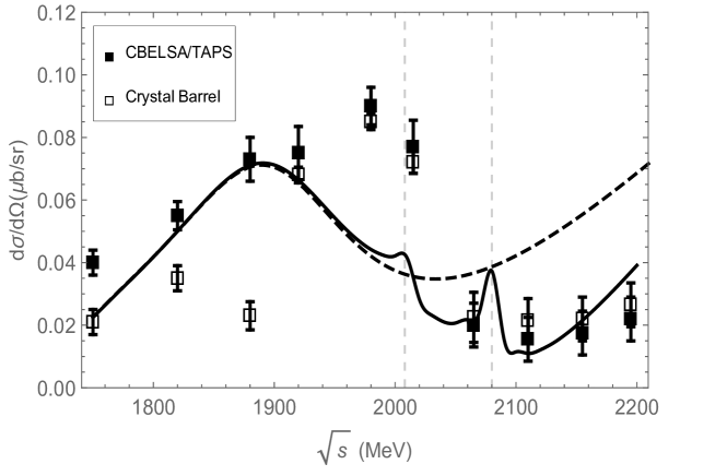
Figure 3: Theoretical results of the differential cross section with respect to CBELSA/TAPS (solid square) and Crystal Barrel Castelijns et al. (2008) (open square). The upper panel shows the result from modified K-MAID (dashed line) with $G1_{\rm S_{31}}(1900)=0.8\,,~{}G1_{\rm P_{31}}(1910)=0.6\,,~{}G2_{\rm S_{31}}(1900)=0.8\,,~{}G2_{\rm P_{31}}(1910)=0.6$ and the cobmined contributions (solid line) of the modified K-MAID model and the imaginary part of the box-diagrams with the best fitted hadronic phases, $\theta_{1}=37.74^{\circ}$ , $\theta_{2}=47.14^{\circ}$ , $\theta_{3}=47.82^{\circ}$. In the lower panel, the dash line is the result contributed by the modified K-MAID, the imaginary part of the box-diagrams, and the $\Delta(1940)$ resonance with the hadronic phases $\theta_{1}=37.74^{\circ}$ , $\theta_{2}=47.14^{\circ}$ , $\theta_{3}=47.82^{\circ}$  while the solid line is the result of the modified K-MAID, the full amplitudes (real and imaginary parts) of the box-diagrams, and the inclusion of the $\Delta(1940)$ resonance.

The CGLN amplitudes $\mathcal{F}_{i}$ for the $\gamma p\,\rightarrow\,K^{0}\Sigma^{+}$ photoproduction process are given by

$$\mathcal{F}_{i}=\alpha\,\mathcal{F}_{i}^{\rm KMAID}+\beta\,\mathcal{F}_{i}^{\Delta(1940)}+\delta\left(e^{i\,\theta_{1}}\,\mathcal{F}_{i}^{\rm box\,(1)}+e^{i\,\theta_{2}}\,\mathcal{F}_{i}^{\rm box\,(2)}+e^{i\,\theta_{3}}\,\mathcal{F}_{i}^{\rm box\,(3)}\right),$$ (43)

where $\mathcal{F}_{i}^{\rm KMAID}$, $\mathcal{F}_{i}^{\Delta(1940)}$ and $\mathcal{F}_{i}^{\rm box\,(1,2,3)}$ are the CGLN amplitudes for the modified K-MAID model, the $\Delta(1940)$ resonance and the imaginary part of the box diagrams 1, 2 and 3 respectively. We have introduced as free parameters the hadronic phases, $\theta_{1,2,3}$ to the box-diagram amplitudes. The parameters are determined by fitting the contributions of the box diagrams to experimental data,

$$\theta_{1}=37.74^{\circ}\,,\qquad\quad\theta_{2}=47.14^{\circ}\,,\qquad\quad\theta_{3}=47.82^{\circ}\,.$$ (44)

In addition, the parameters $\alpha,\,\beta,\,\delta=0,\,1$ are employed as switches to see the contributions of the K-MAID model, $\Delta(1940)$ resonance and box diagrams to the total amplitude respectively.

The numerical result of the imaginary part of the box-diagrams and K-MAID amplitudes are shown in the upper panel of Fig. 3 by setting $\alpha,\delta=1$ and $\beta=0$ . The downfall of the differential cross-section is contributed by the on-shell intermediate $K^{*}\Lambda$ and $K^{*}\Sigma$ states in their mass threshold region. This implies that there are re-scattering effects between the vector kaons and the hyperons in the intermediate states of the processes as depicted in Fig. 2. It is found from Fig. 3, however, that the box-diagram and K-MAID amplitudes can not describe the data from 1920 MeV to the $K^{*}\Lambda$ threshold.

Shown in the lower panel of Fig. 3 are the results including the $\Delta(1940)$ resonance contribution, where the dash line is the result contributed by the modified K-MAID, the imaginary part of the box-diagrams, and the $\Delta(1940)$ resonance with the hadronic phases $\theta_{1}=37.74^{\circ}$ , $\theta_{2}=47.14^{\circ}$ , $\theta_{3}=47.82^{\circ}$  while the solid line is the result contributed together by the modified K-MAID, the full amplitudes (real and imaginary parts) of the box-diagrams, and the $\Delta(1940)$ resonance. One can see that the inclusion of the $\Delta(1940)$ resonance contribution largely raises the differential cross-section, leading to an excellent agreement with the anomaly of the $K^{0}\Sigma^{+}$ photoproduction data.

The bump structure may merely stem from the interference between the amplitudes as the inclusion of the real part of the box-diagrams contributions results in the disappearance of the structure.

IV Conclusions

In this work, we have calculated the contributions of the box-diagrams, the modified K-MAID model, and the $\Delta(1940)$ resonance to the differential cross-section of the photoproduction reaction $\gamma p\,\to\,K^{0}\Sigma^{+}$. The imaginary part of the amplitudes of the box-diagrams is obtained by using the Cutkosky rules while the real part is calculated by using the dispersion relations from the imaginary part of the box-diagram amplitudes. The hadronic phases of the on-shell amplitudes of the box diagrams are introduced as free parameters determined by fitting the theoretical results with the CBELSA/TAPS data.

It is found that the modified K-MAID model provides a good description of the $K^{0}\Sigma^{+}$ photoproduction up to 1920 MeV, and that the inclusion of the $\Delta(1940)$ resonance which contributes via the process $\gamma p\;\rightarrow\;\Delta(1940)\;\rightarrow\,K^{0}\Sigma^{+}$ is necessary to describe the anomaly of the CBELSA/TAPS data.

The work reveals that the theoretical results are sensitive to the property of the $\Delta(1940)$ resonance. Therefore, one may suggest that this two-star resonance may be further investigated in experiments via the $\gamma p\,\to\,K^{0}\Sigma^{+}$ reaction.

Appendix A Extraction of the CGLN amplitudes for $\gamma p\rightarrow K^{0}\Sigma^{+}$ box-diagrams

We give in the section the detailed calculation of the on-shell box-diagrams in the $K^{0}\Sigma^{+}$ photoproduction process. As mentioned earlier, the CGLN amplitudes are invariant amplitude of the photoproduction in the c.m. frame, and can be conveniently incorporated with other sophisticated photoproduction models. The CGLN amplitudes for the box-diagrams shown in Eqs. (II.1.2, II.1.2, II.1.2) will be extracted in the appendix. We start from the most general Lorentz covariant transition matrix element for the photo-production process, which takes the generic form Berends et al. (1967)

$$\mathcal{M} = \bar{u}(\bar{p})\,\sum_{j=1}^{6}B_{j}(s,t,u)\,\epsilon_{\mu}\,N_{j}^{\mu}\,u(p)~{},$$ (45)

where $B_{j}$ are scalar functions and $N_{j}^{\mu}$ are four-vector quantities given by

$$\mathcal{N}_{1}^{\mu} = \gamma_{5}\,\gamma^{\mu}\,k\!\!\!/\,,\quad\mathcal{N}_{2}^{\mu}=2\gamma_{5}\,P^{\mu}\,,\quad\mathcal{N}_{3}^{\mu}=2\gamma_{5}\,q^{\mu}\,,$$

$$\mathcal{N}_{4}^{\mu} = \gamma_{5}\,\gamma^{\mu}\,,\quad\mathcal{N}_{5}^{\mu}=\gamma_{5}\,k\!\!\!/\,P^{\mu}\,,\quad\mathcal{N}_{6}^{\mu}=\gamma_{5}\,k\!\!\!/\,q^{\mu}\,.$$ (46)

One notes that the internal momentum, $l^{\mu}$ always appears in the on-shell amplitudes (II.1.2, II.1.2, II.1.2) and it will appear on the basis $N_{i}^{\mu}$ . To factorize the $l^{\mu}$ momentum out from the basis $N_{i}^{\mu}$, we decompose $l^{\mu}$ in the following way by using Lorentz invariant principle as,

$$l^{\mu} = a\,k^{\mu}+b\,q^{\mu}+c\,p^{\mu}\,,$$ (47)

where $a,~{}b,$  and $c$ are scalar functions, derived as

$$a = -\frac{p^{2}q^{2}k\cdot l-p^{2}k\cdot ql\cdot q-q^{2}k\cdot pl\cdot p-k\cdot l(p\cdot q)^{2}+k\cdot ql\cdot pp\cdot q+k\cdot pl\cdot qp\cdot q}{p^{2}(k\cdot q)^{2}+q^{2}(k\cdot p)^{2}-2k\cdot pk\cdot qp\cdot q},$$

$$b = -\frac{-p^{2}k\cdot lk\cdot q+k\cdot pk\cdot ql\cdot p+(k\cdot p)^{2}(-(l\cdot q))+k\cdot lk\cdot pp\cdot q}{p^{2}(k\cdot q)^{2}+q^{2}(k\cdot p)^{2}-2k\cdot pk\cdot qp\cdot q},$$

$$c = -\frac{-q^{2}k\cdot lk\cdot p+(k\cdot q)^{2}(-(l\cdot p))+k\cdot pk\cdot ql\cdot q+k\cdot lk\cdot qp\cdot q}{p^{2}(k\cdot q)^{2}+q^{2}(k\cdot p)^{2}-2k\cdot pk\cdot qp\cdot q}\,.$$ (48)

In addition, the incoming, $p$, and outgoing, $\bar{p}$, momenta of baryons are also replaced by using the following substitution

$$p^{\mu} = \frac{1}{2}\,\big{(}2\,P^{\mu}+q^{\mu}-k^{\mu}\big{)}\,,$$

$$\bar{p}^{\mu} = \frac{1}{2}\,\big{(}2\,P^{\mu}-q^{\mu}+k^{\mu}\big{)}\,,$$ (49)

where we have defined $P=\frac{1}{2}\,(p+\bar{p})$ .

By using the above definitions for $l^{\mu},~{}p^{\mu}$ and $\bar{p}^{\mu}$ , and substituting to Eqs. (II.1.2,II.1.2,II.1.2), one obtains the decomposition of the amplitudes (II.1.2,II.1.2,II.1.2) in terms of the scalar functions $B_{i}$ defined in Eq. (45) by using the FeynCalc package Mertig et al. (1991); Shtabovenko et al. (2016) in Mathematica. The scalar functions $B_{i}$ are given by

$$B_{1}^{(i)} = \int\rho_{i}\,\Big{\{}-m_{p}m_{V}^{4}-m_{\Sigma}m_{V}^{4}-bm_{p}^{3}m_{V}^{2}-cm_{p}^{3}m_{V}^{2}-bm_{p}m_{\Sigma}^{2}m_{V}^{2}+bm_{Y}m_{\Sigma}^{2}m_{V}^{2}-bm_{K}^{2}m_{p}m_{V}^{2}-cm_{K}^{2}m_{p}m_{V}^{2}$$

$$-\,m_{K}^{2}m_{p}m_{V}^{2}+bk\cdot qm_{p}m_{V}^{2}+ck\cdot qm_{p}m_{V}^{2}+2k\cdot qm_{p}m_{V}^{2}+2ak\cdot\bar{p}m_{p}m_{V}^{2}+2bk\cdot\bar{p}m_{p}m_{V}^{2}+2l\cdot pm_{p}m_{V}^{2}$$

$$+\,bl\cdot qm_{p}m_{V}^{2}+cl\cdot qm_{p}m_{V}^{2}+2l\cdot qm_{p}m_{V}^{2}+2bp\cdot\bar{p}m_{p}m_{V}^{2}+m_{K}^{2}m_{Y}m_{V}^{2}+bm_{p}^{2}m_{Y}m_{V}^{2}+cm_{p}^{2}m_{Y}m_{V}^{2}$$

$$-\,ak\cdot qm_{Y}m_{V}^{2}-bk\cdot qm_{Y}m_{V}^{2}-2k\cdot qm_{Y}m_{V}^{2}-2ak\cdot\bar{p}m_{Y}m_{V}^{2}-2bk\cdot\bar{p}m_{Y}m_{V}^{2}-l\cdot qm_{Y}m_{V}^{2}-2bp\cdot\bar{p}m_{Y}m_{V}^{2}$$

$$-\,bm_{K}^{2}m_{\Sigma}m_{V}^{2}-cm_{p}^{2}m_{\Sigma}m_{V}^{2}-ak\cdot qm_{\Sigma}m_{V}^{2}+2l\cdot pm_{\Sigma}m_{V}^{2}+bl\cdot qm_{\Sigma}m_{V}^{2}+l\cdot qm_{\Sigma}m_{V}^{2}+cm_{p}m_{Y}m_{\Sigma}m_{V}^{2}$$

$$+\,bk\cdot qm_{p}^{3}+ck\cdot qm_{p}^{3}+bl\cdot qm_{p}^{3}+cl\cdot qm_{p}^{3}+bk\cdot qm_{p}m_{\Sigma}^{2}+bl\cdot qm_{p}m_{\Sigma}^{2}-bk\cdot qm_{Y}m_{\Sigma}^{2}-bl\cdot qm_{Y}m_{\Sigma}^{2}$$

$$+\,2bl\cdot pm_{K}^{2}m_{p}+2cl\cdot pm_{K}^{2}m_{p}-2ak\cdot qk\cdot\bar{p}m_{p}-2bk\cdot qk\cdot\bar{p}m_{p}+2ak\cdot ql\cdot pm_{p}-2ck\cdot ql\cdot pm_{p}-2ak\cdot ql\cdot qm_{p}$$

$$-\,2bk\cdot ql\cdot qm_{p}-2k\cdot ql\cdot qm_{p}-2ak\cdot\bar{p}l\cdot qm_{p}-2bk\cdot\bar{p}l\cdot qm_{p}-2bl\cdot pl\cdot qm_{p}-2cl\cdot pl\cdot qm_{p}-2l\cdot pl\cdot qm_{p}$$

$$-\,2bk\cdot qp\cdot\bar{p}m_{p}-2ck\cdot qp\cdot\bar{p}m_{p}-2bl\cdot qp\cdot\bar{p}m_{p}-bk\cdot qm_{p}^{2}m_{Y}-ck\cdot qm_{p}^{2}m_{Y}-bl\cdot qm_{p}^{2}m_{Y}-cl\cdot qm_{p}^{2}m_{Y}$$

$$+\,2ak\cdot qk\cdot\bar{p}m_{Y}+2bk\cdot qk\cdot\bar{p}m_{Y}+2ak\cdot ql\cdot qm_{Y}+2bk\cdot ql\cdot qm_{Y}+2k\cdot ql\cdot qm_{Y}+2ak\cdot\bar{p}l\cdot qm_{Y}$$

$$+\,2bk\cdot\bar{p}l\cdot qm_{Y}+2bk\cdot qp\cdot\bar{p}m_{Y}+2ck\cdot qp\cdot\bar{p}m_{Y}+2bl\cdot qp\cdot\bar{p}m_{Y}+2bl\cdot pm_{K}^{2}m_{\Sigma}-ck\cdot qm_{p}^{2}m_{\Sigma}$$

$$+\,cl\cdot qm_{p}^{2}m_{\Sigma}+2ak\cdot ql\cdot pm_{\Sigma}-2bl\cdot pl\cdot qm_{\Sigma}-2l\cdot pl\cdot qm_{\Sigma}+ck\cdot qm_{p}m_{Y}m_{\Sigma}-cl\cdot qm_{p}m_{Y}m_{\Sigma}$$

$$-\,2(k\cdot l)^{2}\left((a-c)m_{p}+am_{\Sigma}\right)+2k\cdot p\,\big{(}-bm_{p}m_{K}^{2}-cm_{p}m_{K}^{2}-bm_{\Sigma}m_{K}^{2}-am_{p}m_{V}^{2}-bm_{p}m_{V}^{2}-m_{p}m_{V}^{2}$$

$$+\,am_{V}^{2}m_{Y}+bm_{V}^{2}m_{Y}-m_{V}^{2}m_{\Sigma}+l\cdot q\left((a+2b+c+1)m_{p}-(a+b)m_{Y}+(b+1)m_{\Sigma}\right)+k\cdot q\big{(}(b+c)m_{p}$$

$$-\,(a+b)m_{Y}-am_{\Sigma}\big{)}\big{)}+k\cdot l\big{(}bm_{p}^{3}+cm_{p}^{3}-bm_{Y}m_{p}^{2}-cm_{Y}m_{p}^{2}+cm_{\Sigma}m_{p}^{2}+am_{K}^{2}m_{p}+3bm_{K}^{2}m_{p}+2cm_{K}^{2}m_{p}$$

$$+\,m_{K}^{2}m_{p}+am_{V}^{2}m_{p}-cm_{V}^{2}m_{p}+m_{V}^{2}m_{p}+bm_{\Sigma}^{2}m_{p}-2bk\cdot\bar{p}m_{p}-2al\cdot pm_{p}+2cl\cdot pm_{p}-2bl\cdot qm_{p}-2cl\cdot qm_{p}$$

$$-\,4l\cdot qm_{p}-2bp\cdot\bar{p}m_{p}-cm_{Y}m_{\Sigma}m_{p}-bm_{Y}m_{\Sigma}^{2}-am_{K}^{2}m_{Y}-bm_{K}^{2}m_{Y}-m_{K}^{2}m_{Y}+m_{V}^{2}m_{Y}+2bk\cdot\bar{p}m_{Y}$$

$$+\,2l\cdot qm_{Y}+2bp\cdot\bar{p}m_{Y}+2bm_{K}^{2}m_{\Sigma}+am_{V}^{2}m_{\Sigma}+2m_{V}^{2}m_{\Sigma}-2al\cdot pm_{\Sigma}-2bl\cdot qm_{\Sigma}-2l\cdot qm_{\Sigma}$$

$$+\,2k\cdot q\left((a-c)m_{p}+am_{\Sigma}\right)+2k\cdot p\left((a+b)m_{p}-(b+c)m_{Y}+am_{\Sigma}\right)\big{)}\Big{\}}\,,$$

$$B_{2}^{(i)} = \int\rho_{i}\,\frac{1}{2}\,\Big{\{}2k\cdot l\big{(}2bcm_{\Sigma}k\cdot\bar{p}+2bcm_{p}k\cdot\bar{p}+ck\cdot q\left((b+c-2)m_{p}+bm_{\Sigma}\right)-2ck\cdot p\left((b+c)m_{p}+(b-1)m_{\Sigma}\right)$$

$$-\,bm_{K}^{2}m_{Y}+2cm_{p}l\cdot p-cm_{p}m_{V}^{2}-m_{p}m_{V}^{2}+m_{V}^{2}m_{Y}\big{)}+2bcm_{K}^{2}m_{Y}k\cdot\bar{p}-2bcm_{K}^{2}m_{p}k\cdot\bar{p}-2bcm_{\Sigma}k\cdot qk\cdot\bar{p}$$

$$-\,2bcm_{Y}k\cdot qk\cdot\bar{p}-2bcm_{Y}p\cdot\bar{p}k\cdot q+2bcm_{p}p\cdot\bar{p}k\cdot q-4c^{2}m_{p}l\cdot pk\cdot\bar{p}+2c^{2}m_{p}m_{V}^{2}k\cdot\bar{p}-2cm_{V}^{2}m_{Y}k\cdot\bar{p}$$

$$+2cm_{p}m_{V}^{2}k\cdot\bar{p}+2ck\cdot pk\cdot q\left((c-a)m_{p}+(a-c+1)m_{Y}+(c-1)m_{\Sigma}\right)-2bcm_{\Sigma}k\cdot ql\cdot p-2bcm_{p}k\cdot ql\cdot p$$

$$-\,bcm_{p}m_{\Sigma}^{2}k\cdot q+bcm_{p}m_{V}^{2}k\cdot q+bcm_{p}^{2}m_{Y}k\cdot q-bcm_{p}^{3}k\cdot q+bcm_{\Sigma}m_{V}^{2}k\cdot q+bcm_{\Sigma}^{2}m_{Y}k\cdot q-4bm_{p}k\cdot ql\cdot q$$

$$+\,4bm_{Y}k\cdot ql\cdot q+2bm_{p}m_{V}^{2}k\cdot q-2bm_{V}^{2}m_{Y}k\cdot q-2c^{2}m_{p}k\cdot ql\cdot p-c^{2}m_{p}^{2}m_{\Sigma}k\cdot q+c^{2}m_{p}m_{V}^{2}k\cdot q$$

$$+\,c^{2}m_{p}m_{\Sigma}m_{Y}k\cdot q+c^{2}m_{p}^{2}m_{Y}k\cdot q-c^{2}m_{p}^{3}k\cdot q-4c^{2}m_{\Sigma}(k\cdot p)^{2}+2cm_{\Sigma}k\cdot ql\cdot p-2cm_{p}k\cdot ql\cdot p+4cm_{p}(k\cdot l)^{2}$$

$$+\,2cm_{p}m_{V}^{2}k\cdot q-cm_{\Sigma}m_{V}^{2}k\cdot q-cm_{V}^{2}m_{Y}k\cdot q+2m_{p}m_{V}^{2}k\cdot q-2m_{V}^{2}m_{Y}k\cdot q+bm_{K}^{2}m_{p}\Big{\}}\,,$$

$$B_{3}^{(i)} = \int\rho_{i}\,\frac{1}{4}\Big{\{}-2b^{2}k\cdot qm_{p}^{3}-c^{2}k\cdot qm_{p}^{3}-3bck\cdot qm_{p}^{3}+2b^{2}k\cdot qm_{Y}m_{p}^{2}+c^{2}k\cdot qm_{Y}m_{p}^{2}+3bck\cdot qm_{Y}m_{p}^{2}$$

$$-\,2bck\cdot qm_{\Sigma}m_{p}^{2}-4b^{2}k\cdot\bar{p}m_{K}^{2}m_{p}-2bck\cdot\bar{p}m_{K}^{2}m_{p}+2b^{2}k\cdot qm_{V}^{2}m_{p}+c^{2}k\cdot qm_{V}^{2}m_{p}-2bk\cdot qm_{V}^{2}m_{p}$$

$$+\,3bck\cdot qm_{V}^{2}m_{p}-2ck\cdot qm_{V}^{2}m_{p}-2k\cdot qm_{V}^{2}m_{p}+2c^{2}k\cdot\bar{p}m_{V}^{2}m_{p}+4bck\cdot\bar{p}m_{V}^{2}m_{p}-2ck\cdot\bar{p}m_{V}^{2}m_{p}$$

$$-\,2b^{2}k\cdot qm_{\Sigma}^{2}m_{p}-bck\cdot qm_{\Sigma}^{2}m_{p}-4b^{2}k\cdot ql\cdot pm_{p}-2c^{2}k\cdot ql\cdot pm_{p}+4bk\cdot ql\cdot pm_{p}-6bck\cdot ql\cdot pm_{p}$$

$$+\,6ck\cdot ql\cdot pm_{p}-4c^{2}k\cdot\bar{p}l\cdot pm_{p}-8bck\cdot\bar{p}l\cdot pm_{p}+8ck\cdot\bar{p}l\cdot pm_{p}+4bk\cdot ql\cdot qm_{p}+8bk\cdot\bar{p}l\cdot qm_{p}$$

$$+\,4b^{2}k\cdot qp\cdot\bar{p}m_{p}+2bck\cdot qp\cdot\bar{p}m_{p}+c^{2}k\cdot qm_{Y}m_{\Sigma}m_{p}+2bck\cdot qm_{Y}m_{\Sigma}m_{p}+2b^{2}k\cdot qm_{Y}m_{\Sigma}^{2}+bck\cdot qm_{Y}m_{\Sigma}^{2}$$

$$+\,4b^{2}k\cdot\bar{p}m_{K}^{2}m_{Y}+2bck\cdot\bar{p}m_{K}^{2}m_{Y}-ck\cdot qm_{V}^{2}m_{Y}+2k\cdot qm_{V}^{2}m_{Y}-2ck\cdot\bar{p}m_{V}^{2}m_{Y}+4k\cdot\bar{p}m_{V}^{2}m_{Y}$$

$$-\,4b^{2}k\cdot qk\cdot\bar{p}m_{Y}-2bck\cdot qk\cdot\bar{p}m_{Y}-4bk\cdot ql\cdot qm_{Y}-8bk\cdot\bar{p}l\cdot qm_{Y}-4b^{2}k\cdot qp\cdot\bar{p}m_{Y}-2bck\cdot qp\cdot\bar{p}m_{Y}$$

$$-\,4c(2b+c-2)(k\cdot p)^{2}m_{\Sigma}+2b^{2}k\cdot qm_{V}^{2}m_{\Sigma}-2bk\cdot qm_{V}^{2}m_{\Sigma}+bck\cdot qm_{V}^{2}m_{\Sigma}-ck\cdot qm_{V}^{2}m_{\Sigma}-4b^{2}k\cdot qk\cdot\bar{p}m_{\Sigma}$$

$$-\,2bck\cdot qk\cdot\bar{p}m_{\Sigma}-4b^{2}k\cdot ql\cdot pm_{\Sigma}+4bk\cdot ql\cdot pm_{\Sigma}-2bck\cdot ql\cdot pm_{\Sigma}+2ck\cdot ql\cdot pm_{\Sigma}+4b(k\cdot l)^{2}\left(m_{p}+m_{\Sigma}\right)$$

$$+\,2k\cdot pk\cdot q\left(-(a-c)(2b+c)m_{p}+(a-c+1)(2b+c)m_{Y}+(2(c+1)b+(c-1)c)m_{\Sigma}\right)+2k\cdot l\big{(}bm_{p}^{3}+cm_{p}^{3}$$

$$-bm_{Y}m_{p}^{2}-cm_{Y}m_{p}^{2}+cm_{\Sigma}m_{p}^{2}-bm_{K}^{2}m_{p}-bm_{V}^{2}m_{p}+m_{V}^{2}m_{p}+bm_{\Sigma}^{2}m_{p}+4b^{2}k\cdot\bar{p}m_{p}-4bk\cdot\bar{p}m_{p}$$

$$+\,2bck\cdot\bar{p}m_{p}+2bl\cdot pm_{p}-2l\cdot pm_{p}-2bp\cdot\bar{p}m_{p}-cm_{Y}m_{\Sigma}m_{p}-bm_{Y}m_{\Sigma}^{2}+bm_{K}^{2}m_{Y}+2bk\cdot\bar{p}m_{Y}+2bp\cdot\bar{p}m_{Y}$$

$$-\,bm_{V}^{2}m_{\Sigma}+m_{V}^{2}m_{\Sigma}+4b^{2}k\cdot\bar{p}m_{\Sigma}-2bk\cdot\bar{p}m_{\Sigma}+2bck\cdot\bar{p}m_{\Sigma}+2bl\cdot pm_{\Sigma}-2l\cdot pm_{\Sigma}-4k\cdot\bar{p}m_{V}^{2}m_{p}$$

$$+\,k\cdot q\big{(}\left(2b^{2}+(3c-4)b+(c-2)c\right)m_{p}+(2b+c-4)bm_{\Sigma}\big{)}+2k\cdot p\big{(}\left(-2b^{2}-3cb+2b-c^{2}+a+c\right)m_{p}$$

$$+\,(-a+c-1)m_{Y}-\left(2b^{2}+(c-2)b+1\right)m_{\Sigma}\big{)}\big{)}-c^{2}k\cdot qm_{\Sigma}m_{p}^{2}\Big{\}}\,,$$

$$B_{4}^{(i)} = \int\rho_{i}\,\Big{\{}-(k\cdot q)m_{V}^{4}-2k\cdot\bar{p}m_{V}^{4}-2bk\cdot\bar{p}m_{K}^{2}m_{V}^{2}-2bk\cdot qm_{p}^{2}m_{V}^{2}-2ck\cdot qm_{p}^{2}m_{V}^{2}-k\cdot qm_{p}^{2}m_{V}^{2}$$

$$-\,bk\cdot qm_{\Sigma}^{2}m_{V}^{2}+4bk\cdot qk\cdot\bar{p}m_{V}^{2}+2k\cdot ql\cdot pm_{V}^{2}+4k\cdot\bar{p}l\cdot pm_{V}^{2}+2k\cdot ql\cdot qm_{V}^{2}+2bk\cdot\bar{p}l\cdot qm_{V}^{2}$$

$$+\,2k\cdot\bar{p}l\cdot qm_{V}^{2}+2bk\cdot qp\cdot\bar{p}m_{V}^{2}+bk\cdot qm_{p}m_{Y}m_{V}^{2}+ck\cdot qm_{p}m_{Y}m_{V}^{2}+k\cdot qm_{p}m_{Y}m_{V}^{2}+2ck\cdot\bar{p}m_{p}m_{Y}m_{V}^{2}$$

$$+\,bk\cdot qm_{p}m_{\Sigma}m_{V}^{2}+ck\cdot qm_{p}m_{\Sigma}m_{V}^{2}+k\cdot qm_{p}m_{\Sigma}m_{V}^{2}-bk\cdot qm_{Y}m_{\Sigma}m_{V}^{2}-k\cdot qm_{Y}m_{\Sigma}m_{V}^{2}$$

$$+\,4bk\cdot\bar{p}l\cdot pm_{K}^{2}+2bk\cdot ql\cdot pm_{p}^{2}+2ck\cdot ql\cdot pm_{p}^{2}+2bk\cdot ql\cdot qm_{p}^{2}+2ck\cdot ql\cdot qm_{p}^{2}+2ck\cdot\bar{p}l\cdot qm_{p}^{2}$$

$$+\,2bk\cdot ql\cdot pm_{\Sigma}^{2}-4bk\cdot qk\cdot\bar{p}l\cdot p-4k\cdot ql\cdot pl\cdot q-4bk\cdot\bar{p}l\cdot pl\cdot q-4k\cdot\bar{p}l\cdot pl\cdot q-2ck\cdot\bar{p}m_{p}^{2}m_{V}^{2}$$

$$+\,4(k\cdot p)^{2}\left(-bm_{K}^{2}-cm_{K}^{2}-m_{V}^{2}+(b+c)k\cdot q+(b+c+1)l\cdot q\right)-4bk\cdot ql\cdot pp\cdot\bar{p}-2(k\cdot l)^{2}\big{(}bm_{p}^{2}+cm_{p}^{2}$$

$$-\,cm_{\Sigma}m_{p}+bm_{\Sigma}^{2}+2(a+b)k\cdot p-2bk\cdot\bar{p}-2bp\cdot\bar{p}\big{)}+k\cdot l\big{(}4(a+b)(k\cdot p)^{2}+2\big{(}bm_{K}^{2}+cm_{K}^{2}+m_{K}^{2}+bm_{p}^{2}$$

$$+\,cm_{p}^{2}+am_{V}^{2}+bm_{V}^{2}+2m_{V}^{2}+bm_{\Sigma}^{2}+2(a+b)k\cdot q-cm_{K}^{2}m_{p}^{2}-2bl\cdot pm_{p}^{2}$$

$$-\,2bk\cdot\bar{p}-2al\cdot p-2bl\cdot p-4l\cdot q-2bp\cdot\bar{p}-cm_{Y}m_{\Sigma}\big{)}k\cdot p+2bk\cdot\bar{p}m_{K}^{2}+2l\cdot pm_{K}^{2}-bm_{K}^{2}m_{p}^{2}$$

$$-\,2cl\cdot pm_{p}^{2}-m_{K}^{2}m_{V}^{2}+bm_{p}^{2}m_{V}^{2}+cm_{p}^{2}m_{V}^{2}+m_{p}^{2}m_{V}^{2}-2bk\cdot\bar{p}m_{V}^{2}-2bp\cdot\bar{p}m_{V}^{2}+bm_{V}^{2}m_{\Sigma}^{2}-2bl\cdot pm_{\Sigma}^{2}$$

$$+\,4bk\cdot\bar{p}l\cdot p-4bk\cdot\bar{p}l\cdot q+4bl\cdot pp\cdot\bar{p}+2k\cdot q\left(bm_{p}^{2}+cm_{p}^{2}-cm_{\Sigma}m_{p}+bm_{\Sigma}^{2}-2bk\cdot\bar{p}-2bp\cdot\bar{p}\right)$$

$$-\,m_{p}m_{V}^{2}m_{Y}+bm_{K}^{2}m_{p}m_{Y}+cm_{K}^{2}m_{p}m_{Y}-cm_{p}m_{V}^{2}m_{\Sigma}-m_{p}m_{V}^{2}m_{\Sigma}+bm_{K}^{2}m_{p}m_{\Sigma}+2cl\cdot pm_{p}m_{\Sigma}$$

$$-\,bm_{K}^{2}m_{Y}m_{\Sigma}+m_{V}^{2}m_{Y}m_{\Sigma}\big{)}-2bk\cdot ql\cdot qm_{p}m_{Y}-2ck\cdot ql\cdot qm_{p}m_{Y}-2ck\cdot\bar{p}l\cdot qm_{p}m_{Y}$$

$$-\,2ck\cdot ql\cdot pm_{p}m_{\Sigma}-2bk\cdot ql\cdot qm_{p}m_{\Sigma}+2bk\cdot ql\cdot qm_{Y}m_{\Sigma}$$

$$-\,2k\cdot pk\cdot q\big{(}-bm_{p}^{2}-cm_{p}^{2}+am_{V}^{2}+2bm_{V}^{2}+cm_{V}^{2}-m_{V}^{2}-bm_{\Sigma}^{2}+2(a+b)k\cdot\bar{p}-2(a+b)l\cdot p+2l\cdot q$$

$$+\,2bp\cdot\bar{p}+2cp\cdot\bar{p}-cm_{Y}m_{\Sigma}\big{)}\Big{\}}\,,$$

$$B_{5}^{(i)} = \int\rho_{i}\,\Big{\{}2m_{V}^{4}+2bm_{K}^{2}m_{V}^{2}+cm_{K}^{2}m_{V}^{2}-c^{2}m_{p}^{2}m_{V}^{2}-bcm_{p}^{2}m_{V}^{2}+cm_{p}^{2}m_{V}^{2}-bcm_{\Sigma}^{2}m_{V}^{2}+2ak\cdot qm_{V}^{2}$$

$$+\,bck\cdot qm_{V}^{2}-ck\cdot qm_{V}^{2}+2ack\cdot\bar{p}m_{V}^{2}+2bck\cdot\bar{p}m_{V}^{2}-4l\cdot pm_{V}^{2}-2bl\cdot qm_{V}^{2}-2l\cdot qm_{V}^{2}+2bcp\cdot\bar{p}m_{V}^{2}$$

$$-\,cm_{p}m_{Y}m_{V}^{2}+c^{2}m_{p}m_{\Sigma}m_{V}^{2}+cm_{p}m_{\Sigma}m_{V}^{2}-cm_{Y}m_{\Sigma}m_{V}^{2}+4a(k\cdot l)^{2}-4c(b+c)(k\cdot p)^{2}-4bl\cdot pm_{K}^{2}$$

$$-\,2cl\cdot pm_{K}^{2}+c^{2}m_{K}^{2}m_{p}^{2}+bcm_{K}^{2}m_{p}^{2}-2c^{2}k\cdot qm_{p}^{2}+ack\cdot qm_{p}^{2}-bck\cdot qm_{p}^{2}+ck\cdot qm_{p}^{2}+2c^{2}l\cdot pm_{p}^{2}$$

$$+\,2bcl\cdot pm_{p}^{2}-2cl\cdot qm_{p}^{2}+2bcl\cdot pm_{\Sigma}^{2}-2bck\cdot qk\cdot\bar{p}-4ak\cdot ql\cdot p-2ack\cdot ql\cdot p-2bck\cdot ql\cdot p$$

$$+\,2ck\cdot ql\cdot p-4ack\cdot\bar{p}l\cdot p-4bck\cdot\bar{p}l\cdot p+4bl\cdot pl\cdot q+4l\cdot pl\cdot q+ack\cdot qm_{V}^{2}-2k\cdot p\big{(}m_{p}^{2}c^{2}-m_{p}m_{\Sigma}c^{2}$$

$$-\,m_{K}^{2}c+bm_{p}^{2}c+am_{V}^{2}c+bm_{V}^{2}c+bm_{\Sigma}^{2}c-2bk\cdot\bar{p}c-2al\cdot pc-2bl\cdot pc-2bp\cdot\bar{p}c-2bm_{K}^{2}$$

$$-\,2m_{V}^{2}+(a(c-2)-(c-1)c)k\cdot q+2bl\cdot q+2l\cdot q\big{)}+2k\cdot l\big{(}m_{p}^{2}c^{2}-m_{p}m_{\Sigma}c^{2}-m_{K}^{2}c+bm_{p}^{2}c+bm_{\Sigma}^{2}c$$

$$-\,2bp\cdot\bar{p}c-m_{p}m_{\Sigma}c+m_{Y}m_{\Sigma}c-2bm_{K}^{2}-am_{V}^{2}-2m_{V}^{2}-2(a-c)k\cdot p+((c-2)a+bc)k\cdot q+2al\cdot p$$

$$+\,2bl\cdot q+2l\cdot q\big{)}-4bcl\cdot pp\cdot\bar{p}-c^{2}m_{K}^{2}m_{p}m_{Y}-bcm_{K}^{2}m_{p}m_{Y}+2c^{2}k\cdot qm_{p}m_{Y}-ack\cdot qm_{p}m_{Y}$$

$$+\,2cl\cdot qm_{p}m_{Y}-bcm_{K}^{2}m_{p}m_{\Sigma}-ack\cdot qm_{p}m_{\Sigma}+bck\cdot qm_{p}m_{\Sigma}+ck\cdot qm_{p}m_{\Sigma}-2c^{2}l\cdot pm_{p}m_{\Sigma}$$

$$+\,bcm_{K}^{2}m_{Y}m_{\Sigma}+ack\cdot qm_{Y}m_{\Sigma}-bck\cdot qm_{Y}m_{\Sigma}-ck\cdot qm_{Y}m_{\Sigma}+bck\cdot qm_{p}m_{Y}-ck\cdot qm_{p}m_{Y}\Big{\}}\,,$$

$$B_{6}^{(i)} = \int\rho_{i}\,\frac{1}{2}\Big{\{}2m_{K}^{2}m_{p}^{2}b^{2}-2k\cdot qm_{p}^{2}b^{2}+4l\cdot pm_{p}^{2}b^{2}-2m_{p}^{2}m_{V}^{2}b^{2}+2k\cdot qm_{V}^{2}b^{2}+4k\cdot\bar{p}m_{V}^{2}b^{2}+4p\cdot\bar{p}m_{V}^{2}b^{2}$$ (50)

$$+\,4l\cdot pm_{\Sigma}^{2}b^{2}-4k\cdot qk\cdot\bar{p}b^{2}-4k\cdot ql\cdot pb^{2}-8k\cdot\bar{p}l\cdot pb^{2}-8l\cdot pp\cdot\bar{p}b^{2}-2m_{K}^{2}m_{p}m_{Y}b^{2}+2k\cdot qm_{p}m_{Y}b^{2}$$

$$-\,2m_{K}^{2}m_{p}m_{\Sigma}b^{2}+2k\cdot qm_{p}m_{\Sigma}b^{2}+2m_{K}^{2}m_{Y}m_{\Sigma}b^{2}-2k\cdot qm_{Y}m_{\Sigma}b^{2}+4(k\cdot l)^{2}b+3cm_{K}^{2}m_{p}^{2}b+2ak\cdot qm_{p}^{2}b$$

$$-\,5ck\cdot qm_{p}^{2}b+2k\cdot qm_{p}^{2}b+6cl\cdot pm_{p}^{2}b-4l\cdot pm_{p}^{2}b-4l\cdot qm_{p}^{2}b-3cm_{p}^{2}m_{V}^{2}b+2m_{p}^{2}m_{V}^{2}b+2ak\cdot qm_{V}^{2}b+ck\cdot qm_{V}^{2}b$$

$$-\,2k\cdot qm_{V}^{2}b+4ak\cdot\bar{p}m_{V}^{2}b+2ck\cdot\bar{p}m_{V}^{2}b-4k\cdot\bar{p}m_{V}^{2}b+2l\cdot qm_{V}^{2}b+2cp\cdot\bar{p}m_{V}^{2}b-4p\cdot\bar{p}m_{V}^{2}b-cm_{V}^{2}m_{\Sigma}^{2}b$$

$$+\,2m_{V}^{2}m_{\Sigma}^{2}b+2cl\cdot pm_{\Sigma}^{2}b-4l\cdot pm_{\Sigma}^{2}b-2ck\cdot qk\cdot\bar{p}b-4ak\cdot ql\cdot pb-2ck\cdot ql\cdot pb+4k\cdot ql\cdot pb-8ak\cdot\bar{p}l\cdot pb$$

$$-\,4ck\cdot\bar{p}l\cdot pb+8k\cdot\bar{p}l\cdot pb-4l\cdot pl\cdot qb-4cl\cdot pp\cdot\bar{p}b+8l\cdot pp\cdot\bar{p}b-3cm_{K}^{2}m_{p}m_{Y}b-2ak\cdot qm_{p}m_{Y}b$$

$$+\,5ck\cdot qm_{p}m_{Y}b-2k\cdot qm_{p}m_{Y}b+4l\cdot qm_{p}m_{Y}b+2cm_{p}m_{V}^{2}m_{\Sigma}b-cm_{K}^{2}m_{p}m_{\Sigma}b-2ak\cdot qm_{p}m_{\Sigma}b$$

$$+\,ck\cdot qm_{p}m_{\Sigma}b-2k\cdot qm_{p}m_{\Sigma}b-4cl\cdot pm_{p}m_{\Sigma}b+4l\cdot qm_{p}m_{\Sigma}b+cm_{K}^{2}m_{Y}m_{\Sigma}b+2ak\cdot qm_{Y}m_{\Sigma}b$$

$$-\,ck\cdot qm_{Y}m_{\Sigma}b+2k\cdot qm_{Y}m_{\Sigma}b-4l\cdot qm_{Y}m_{\Sigma}b-4\left(2b^{2}+(3c+2)b+c^{2}+2a\right)(k\cdot p)^{2}-2m_{V}^{2}m_{\Sigma}^{2}b^{2}$$

$$-\,2cl\cdot pm_{K}^{2}+c^{2}m_{K}^{2}m_{p}^{2}-2c^{2}k\cdot qm_{p}^{2}+ack\cdot qm_{p}^{2}+ck\cdot qm_{p}^{2}+2c^{2}l\cdot pm_{p}^{2}-4cl\cdot pm_{p}^{2}-2cl\cdot qm_{p}^{2}+cm_{K}^{2}m_{V}^{2}$$

$$-\,c^{2}m_{p}^{2}m_{V}^{2}+cm_{p}^{2}m_{V}^{2}+2m_{p}^{2}m_{V}^{2}-2ak\cdot qm_{V}^{2}+ack\cdot qm_{V}^{2}-ck\cdot qm_{V}^{2}-4ak\cdot\bar{p}m_{V}^{2}+2ack\cdot\bar{p}m_{V}^{2}-2l\cdot qm_{V}^{2}$$

$$+\,4ak\cdot ql\cdot p-2ack\cdot ql\cdot p+2ck\cdot ql\cdot p+8ak\cdot\bar{p}l\cdot p-4ack\cdot\bar{p}l\cdot p+4l\cdot pl\cdot q+cm_{p}m_{V}^{2}m_{Y}-2m_{p}m_{V}^{2}m_{Y}$$

$$-\,c^{2}m_{K}^{2}m_{p}m_{Y}+2c^{2}k\cdot qm_{p}m_{Y}-ack\cdot qm_{p}m_{Y}-ck\cdot qm_{p}m_{Y}+2cl\cdot qm_{p}m_{Y}+c^{2}m_{p}m_{V}^{2}m_{\Sigma}-cm_{p}m_{V}^{2}m_{\Sigma}$$

$$-\,2m_{p}m_{V}^{2}m_{\Sigma}-ack\cdot qm_{p}m_{\Sigma}+ck\cdot qm_{p}m_{\Sigma}-2c^{2}l\cdot pm_{p}m_{\Sigma}+4cl\cdot pm_{p}m_{\Sigma}-cm_{V}^{2}m_{Y}m_{\Sigma}+2m_{V}^{2}m_{Y}m_{\Sigma}$$

$$+\,ack\cdot qm_{Y}m_{\Sigma}-ck\cdot qm_{Y}m_{\Sigma}-2k\cdot l\big{(}-2m_{p}^{2}b^{2}-2m_{\Sigma}^{2}b^{2}+4p\cdot\bar{p}b^{2}-3cm_{p}^{2}b+m_{p}^{2}b+m_{V}^{2}b-cm_{\Sigma}^{2}b+2m_{\Sigma}^{2}b$$

$$-\,2k\cdot\bar{p}b-2l\cdot pb+2l\cdot qb+2cp\cdot\bar{p}b-4p\cdot\bar{p}b+m_{p}m_{Y}b+2cm_{p}m_{\Sigma}b+m_{p}m_{\Sigma}b-m_{Y}m_{\Sigma}b+cm_{K}^{2}-c^{2}m_{p}^{2}+am_{p}^{2}$$

$$+\,m_{p}^{2}-m_{V}^{2}+2k\cdot p-((2b+c-2)a+(2b+c-4)b)k\cdot q+2l\cdot p-2l\cdot q-am_{p}m_{Y}+2cm_{p}m_{Y}-m_{p}m_{Y}$$

$$+\,c^{2}m_{p}m_{\Sigma}-am_{p}m_{\Sigma}-cm_{p}m_{\Sigma}-m_{p}m_{\Sigma}+am_{Y}m_{\Sigma}-cm_{Y}m_{\Sigma}+m_{Y}m_{\Sigma}\big{)}+2k\cdot p\big{(}-2m_{p}^{2}b^{2}-2m_{V}^{2}b^{2}$$

$$-\,2m_{\Sigma}^{2}b^{2}+4l\cdot pb^{2}+4p\cdot\bar{p}b^{2}-3cm_{p}^{2}b-2m_{p}^{2}b-2am_{V}^{2}b-cm_{V}^{2}b+2m_{V}^{2}b-cm_{\Sigma}^{2}b-2m_{\Sigma}^{2}b+4al\cdot pb+2cl\cdot pb$$

$$-\,4l\cdot pb+2l\cdot qb+2cp\cdot\bar{p}b+4p\cdot\bar{p}b+2cm_{p}m_{\Sigma}b+cm_{K}^{2}-c^{2}m_{p}^{2}-2cm_{p}^{2}+2am_{V}^{2}-acm_{V}^{2}$$

$$+\,(-(2b+c-2)a+2(c+1)b+(c-1)c)k\cdot q+2(2a+(2b+c+2)b)k\cdot\bar{p}-4al\cdot p+2acl\cdot p+2l\cdot q$$

$$+\,4cp\cdot\bar{p}+c^{2}m_{p}m_{\Sigma}-2cm_{p}m_{\Sigma}\big{)}\Big{\}}\,,$$

where we have defined the notation $\int\rho_{i}$ as

$$\int\rho_{i}=\frac{\widetilde{l}}{32\,\pi^{2}\,\sqrt{s}}\,G_{i}\int d\,\Omega\;\frac{F_{K}^{2}(k-l)}{(k-l)^{2}-m_{\bar{K}}^{2}}\,\frac{F_{\pi}^{2}(l-q)}{(l-q)^{2}-m_{\pi}^{2}}\,.$$ (51)

In addition, the following identities are applied for factorizing the $B_{i}^{(j)}$ functions,

$$l^{\mu} = l_{\nu}\,g^{\mu\nu}=\frac{1}{2}\,(\gamma^{\mu}\,l\!\!\!/+l\!\!\!/\,\gamma^{\mu})\,,$$ (52)

$$\epsilon^{\mu\nu\alpha\beta}\,\gamma_{\beta} = i\,(g^{\mu\nu}\,\gamma^{\alpha}-g^{\mu\alpha}\,\gamma^{\nu}+g^{\nu\alpha}\,\gamma^{\mu}-\gamma^{\mu}\,\gamma^{\nu}\,\gamma^{\alpha})\,\gamma_{5}\,.$$

The photoproduction amplitude $\mathcal{M}$ is conventionally decomposed into the gauge- and Lorentz-invariant matrices $M_{i}$ where we have used the convention in Refs. Berends et al. (1967). The $\mathcal{M}$ can be written as

$$\mathcal{M} = \bar{u}(\bar{p})\,\sum_{j=1}^{4}A_{j}(s,t,u)\,M_{j}\,u(p)~{},$$ (53)

where $s$ and $t$ are the usual Mandelstam variables, defined by

$$s=(k+p)^{2},~{}~{}t=(k-q)^{2},~{}~{}u~{}=~{}(k-\bar{p})^{2}~{},$$ (54)

The gauge and Lorentz invariant matrices $M_{j}$ are given by

$$M_{1} = {\textstyle\frac{1}{2}}\,\gamma_{5}\,\big{\{}\epsilon\!\!\!/\,k\!\!\!/-k\!\!\!/\,\epsilon\!\!\!/\big{\}}~{},$$

$$M_{2} = 2\,\gamma_{5}\,\big{\{}(q\cdot\epsilon)\,(P\cdot k)-(q\cdot k)\,(P\cdot\epsilon)\big{\}}~{},$$

$$M_{3} = \gamma_{5}\,\big{\{}(q\cdot k)\,\epsilon\!\!\!/-(q\cdot\epsilon)\,k\!\!\!/\big{\}}~{},$$ (55)

$$M_{4} = 2\,\gamma_{5}\,\big{\{}(P\cdot k)\,\epsilon\!\!\!/-(P\cdot\epsilon)\,k\!\!\!/\big{\}}-(m_{p}+m_{\Sigma})\,M_{1}\,,$$

where $P=\frac{1}{2}(p+\bar{p})$, and $\epsilon_{\mu\nu\rho\sigma}$ is the four dimensional Levi-Civita tensor with $\epsilon_{0123}=+1$.

By imposing the gauge invariant condition, $k^{\mu}\epsilon_{\mu}^{(\gamma)}(k)=0$, the $A_{i}$ are rewritten in terms of the scalar function $B_{i}$ via the following relations Berends et al. (1967),

$$A_{1} = B_{1}-\frac{1}{2}\,(m_{p}+m_{\Sigma})\,B_{5}\,,$$

$$A_{2} = \frac{2\,B_{2}}{M_{K}^{2}-t}\,,$$

$$A_{3} = -B_{6}\,,$$

$$A_{4} = -\frac{1}{2}B_{5}\,.$$ (56)

By using above relations, we obtain invariant amplitudes in terms of the Lorentz covariant and gauge invariant manners. However, this form of the Lorentz covariant fashion is not convenient for the non-relativistic calculation, e.g. photoproduction amplitudes form quark models. Then, we further proceed to extract the CGLN amplitudes which are defined by the following decomposition, Chew et al. (1957)

$$\mathcal{F}=\mathcal{F}_{1}\,\vec{\sigma}\cdot\vec{\varepsilon}+\mathcal{F}_{2}\,i\,(\vec{\sigma}\cdot\hat{q}\,)\,(\vec{\varepsilon}\times\hat{k}\,)\cdot\,\vec{\sigma}+\mathcal{F}_{3}\,(\vec{\sigma}\cdot\hat{k}\,)\,(\hat{q}\cdot\vec{\varepsilon}\,)+\mathcal{F}_{4}\,(\vec{\sigma}\cdot\hat{q}\,)\,(\hat{q}\cdot\vec{\varepsilon}\,)\,,$$ (57)

Therefore, the scalar functions, $\mathcal{F}_{j}$ of the CGLN amplitudes are given in terms of $A_{j}$ functions by Mart et al. (2015)

$$\mathcal{F}_{1,2} = \frac{1}{8\,\pi\,W}\,\sqrt{(E_{p}\mp m_{p})\,(E_{\Sigma}\pm m_{\Sigma})}\,\Big{[}\pm\,(W\mp m_{p})\,A_{1}+\vec{q}\cdot\vec{k}\,(A_{3}-A_{4})+(W\mp m_{p})\,(W\mp m_{\Sigma})\,A_{4}\Big{]}\,,$$ (58)

$$\mathcal{F}_{3,4} = \frac{\widetilde{q}\,\widetilde{k}}{8\,\pi\,W}\,\sqrt{\frac{(E_{\Sigma}\pm m_{\Sigma})}{(E_{p}\mp m_{p})}}\,\Big{[}\pm\,(s-m_{p}^{2})\,A_{2}+(W\mp m_{p})\,(A_{3}-A_{4})\Big{]}\,.$$ (59)

The CGLN amplitudes of the on-shell box-diagrams are obtained in the analytical forms, and ready for numerical integrations as mentioned in Section III.

References

- Hey and Kelly (1983) A. J. G. Hey and R. L. Kelly, Phys. Rept. 96, 71 (1983).
- Glozman (1996) L. Ya. Glozman, Quarks in hadrons and nuclei. Proceedings, International School of Nuclear Physics, Erice, Italy, September 19-27, 1995, Prog. Part. Nucl. Phys. 36, 275 (1996), arXiv:hep-ph/9511418 [hep-ph] .
- Anisovich et al. (2007) A. V. Anisovich, V. Kleber, E. Klempt, V. A. Nikonov, A. V. Sarantsev, and U. Thoma, Eur. Phys. J. A34, 243 (2007), arXiv:0707.3596 [hep-ph] .
- Klempt and Richard (2010) E. Klempt and J.-M. Richard, Rev. Mod. Phys. 82, 1095 (2010), arXiv:0901.2055 [hep-ph] .
- Aznauryan and Burkert (2012) I. G. Aznauryan and V. D. Burkert, Prog. Part. Nucl. Phys. 67, 1 (2012), arXiv:1109.1720 [hep-ph] .
- Crede and Roberts (2013) V. Crede and W. Roberts, Rept. Prog. Phys. 76, 076301 (2013), arXiv:1302.7299 [nucl-ex] .
- Kaiser et al. (1997) N. Kaiser, T. Waas, and W. Weise, Nucl. Phys. A612, 297 (1997), arXiv:hep-ph/9607459 [hep-ph] .
- Nacher et al. (1999) J. C. Nacher, E. Oset, H. Toki, and A. Ramos, Phys. Lett. B455, 55 (1999), arXiv:nucl-th/9812055 [nucl-th] .
- Soyeur and Lutz (2005) M. Soyeur and M. F. M. Lutz, Lepton scattering and the structure of hadrons and nuclei. Proceedings, International School of nuclear physics, 26th Course, Erice, Italy, September 16-24, 2004, Prog. Part. Nucl. Phys. 55, 165 (2005), arXiv:nucl-th/0412027 [nucl-th] .
- Liu et al. (2008) X.-H. Liu, Q. Zhao, and F. E. Close, Phys. Rev. D77, 094005 (2008), arXiv:0802.2648 [hep-ph] .
- Wang et al. (2015) Q. Wang, X.-H. Liu, and Q. Zhao, Phys. Rev. D92, 034022 (2015), arXiv:1508.00339 [hep-ph] .
- Chen et al. (2016) H.-X. Chen, W. Chen, X. Liu, and S.-L. Zhu, Phys. Rept. 639, 1 (2016), arXiv:1601.02092 [hep-ph] .
- Guo et al. (2018) F.-K. Guo, C. Hanhart, U.-G. Meißner, Q. Wang, Q. Zhao, and B.-S. Zou, Rev. Mod. Phys. 90, 015004 (2018), arXiv:1705.00141 [hep-ph] .
- Liu et al. (2019) Y.-R. Liu, H.-X. Chen, W. Chen, X. Liu, and S.-L. Zhu, Prog. Part. Nucl. Phys. 107, 237 (2019), arXiv:1903.11976 [hep-ph] .
- Kroll and Ruderman (1954) N. M. Kroll and M. A. Ruderman, Phys. Rev. 93, 233 (1954).
- Chew et al. (1957) G. F. Chew, M. L. Goldberger, F. E. Low, and Y. Nambu, Phys. Rev. 106, 1345 (1957).
- Dalitz et al. (1967) R. H. Dalitz, T. C. Wong, and G. Rajasekaran, Phys. Rev. 153, 1617 (1967).
- Thom (1966) H. Thom, Phys. Rev. 151, 1322 (1966).
- Berends et al. (1967) F. A. Berends, A. Donnachie, and D. L. Weaver, Nucl. Phys. B4, 1 (1967).
- Walker (1969) R. L. Walker, Phys. Rev. 182, 1729 (1969).
- Adelseck et al. (1985) R. A. Adelseck, C. Bennhold, and L. E. Wright, Phys. Rev. C32, 1681 (1985).
- Workman (1989) R. L. Workman, Phys. Rev. C40, 2922 (1989).
- Adelseck and Saghai (1990) R. A. Adelseck and B. Saghai, Phys. Rev. C42, 108 (1990).
- Drechsel and Tiator (1992) D. Drechsel and L. Tiator, J. Phys. G18, 449 (1992).
- Steininger and Meissner (1997) S. Steininger and U.-G. Meissner, Phys. Lett. B391, 446 (1997), arXiv:nucl-th/9609051 [nucl-th] .
- Guidal et al. (1997) M. Guidal, J. M. Laget, and M. Vanderhaeghen, Nucl. Phys. A627, 645 (1997).
- Borasoy et al. (2007) B. Borasoy, P. C. Bruns, U.-G. Meissner, and R. Nissler, Eur. Phys. J. A34, 161 (2007), arXiv:0709.3181 [nucl-th] .
- Julia-Diaz et al. (2008) B. Julia-Diaz, T. S. H. Lee, A. Matsuyama, T. Sato, and L. C. Smith, Phys. Rev. C77, 045205 (2008), arXiv:0712.2283 [nucl-th] .
- Huang et al. (2012) F. Huang, M. Doring, H. Haberzettl, J. Haidenbauer, C. Hanhart, S. Krewald, U. G. Meissner, and K. Nakayama, Phys. Rev. C85, 054003 (2012), arXiv:1110.3833 [nucl-th] .
- Ronchen et al. (2013) D. Ronchen, M. Doring, F. Huang, H. Haberzettl, J. Haidenbauer, C. Hanhart, S. Krewald, U. G. Meissner, and K. Nakayama, Eur. Phys. J. A49, 44 (2013), arXiv:1211.6998 [nucl-th] .
- Copley et al. (1969) L. A. Copley, G. Karl, and E. Obryk, Nucl. Phys. B13, 303 (1969).
- Li (1995) Z.-P. Li, Phys. Rev. C52, 1648 (1995), arXiv:hep-ph/9502218 [hep-ph] .
- Li et al. (1997) Z.-p. Li, H.-x. Ye, and M.-h. Lu, Phys. Rev. C56, 1099 (1997), arXiv:nucl-th/9706010 [nucl-th] .
- Zhao et al. (2002) Q. Zhao, J. S. Al-Khalili, Z. P. Li, and R. L. Workman, Phys. Rev. C65, 065204 (2002), arXiv:nucl-th/0202067 [nucl-th] .
- Zhong and Zhao (2011) X.-H. Zhong and Q. Zhao, Phys. Rev. C84, 045207 (2011), arXiv:1106.2892 [nucl-th] .
- Knochlein et al. (1995) G. Knochlein, D. Drechsel, and L. Tiator, Z. Phys. A352, 327 (1995), arXiv:nucl-th/9506029 [nucl-th] .
- Drechsel et al. (1999) D. Drechsel, O. Hanstein, S. S. Kamalov, and L. Tiator, Nucl. Phys. A645, 145 (1999), arXiv:nucl-th/9807001 [nucl-th] .
- Kamalov et al. (2001) S. S. Kamalov, S. N. Yang, D. Drechsel, O. Hanstein, and L. Tiator, Phys. Rev. C64, 032201 (2001), arXiv:nucl-th/0006068 [nucl-th] .
- Chiang et al. (2002) W.-T. Chiang, S.-N. Yang, L. Tiator, and D. Drechsel, Nucl. Phys. A700, 429 (2002), arXiv:nucl-th/0110034 [nucl-th] .
- Chiang et al. (2003) W.-T. Chiang, S. N. Yang, L. Tiator, M. Vanderhaeghen, and D. Drechsel, Phys. Rev. C68, 045202 (2003), arXiv:nucl-th/0212106 [nucl-th] .
- Drechsel et al. (2007) D. Drechsel, S. S. Kamalov, and L. Tiator, Eur. Phys. J. A34, 69 (2007), arXiv:0710.0306 [nucl-th] .
- Hilt et al. (2013) M. Hilt, B. C. Lehnhart, S. Scherer, and L. Tiator, Phys. Rev. C88, 055207 (2013), arXiv:1309.3385 [nucl-th] .
- Tiator et al. (2011) L. Tiator, D. Drechsel, S. S. Kamalov, and M. Vanderhaeghen, Eur. Phys. J. ST 198, 141 (2011), arXiv:1109.6745 [nucl-th] .
- Tiator (2018) L. Tiator, Proceedings, 11th International Workshop on the Physics of Excited Nucleons (NSTAR 2017): Columbia, SC, USA, August 20-23, 2017, Few Body Syst. 59, 21 (2018), arXiv:1801.04777 [nucl-th] .
- Lee et al. (2001) F. X. Lee, T. Mart, C. Bennhold, and L. E. Wright, Nucl. Phys. A695, 237 (2001), arXiv:nucl-th/9907119 [nucl-th] .
- Mart and Bennhold (2000) T. Mart and C. Bennhold, Phys. Rev. C61, 012201 (2000), arXiv:nucl-th/9906096 [nucl-th] .
- Bennhold et al. (2000) C. Bennhold, A. Waluyo, H. Haberzettl, T. Mart, G. Penner, and U. Mosel, in In *Newport News 2000, Excited nucleons and hadronic structure* 280-287 (2000) pp. 280–287, arXiv:nucl-th/0008024 [nucl-th] .
- Bennhold et al. (1999) C. Bennhold, H. Haberzettl, and T. Mart, in Perspectives in hadronic physics. Proceedings, 2nd International Conference, Trieste, Italy, May 10-14, 1999 (1999) pp. 328–337, arXiv:nucl-th/9909022 [nucl-th] .
- Ewald et al. (2012) R. Ewald et al. (CBELSA/TAPS), Phys. Lett. B713, 180 (2012), arXiv:1112.0811 [nucl-ex] .
- Castelijns et al. (2008) R. Castelijns et al. (CBELSA/TAPS), Eur. Phys. J. A35, 39 (2008), arXiv:nucl-ex/0702033 [NUCL-EX] .
- Ramos and Oset (2013) A. Ramos and E. Oset, Phys. Lett. B727, 287 (2013), arXiv:1304.7975 [nucl-th] .
- Hyodo et al. (2004) T. Hyodo, A. Hosaka, M. J. Vicente Vacas, and E. Oset, Phys. Lett. B593, 75 (2004), arXiv:nucl-th/0401051 [nucl-th] .
- Oh et al. (2004) Y.-s. Oh, H.-c. Kim, and S. H. Lee, Phys. Rev. D69, 014009 (2004), arXiv:hep-ph/0310019 [hep-ph] .
- Palomar and Oset (2003) J. E. Palomar and E. Oset, Nucl. Phys. A716, 169 (2003), arXiv:nucl-th/0208013 [nucl-th] .
- Chiang et al. (2004) W.-T. Chiang, B. Saghai, F. Tabakin, and T. S. H. Lee, Phys. Rev. C69, 065208 (2004), arXiv:nucl-th/0404062 [nucl-th] .
- Peskin and Schroeder (1995) M. E. Peskin and D. V. Schroeder, An Introduction to quantum field theory (Addison-Wesley, Reading, USA, 1995).
- Usov and Scholten (2005) A. Usov and O. Scholten, Phys. Rev. C72, 025205 (2005), arXiv:nucl-th/0503013 [nucl-th] .
- Guo et al. (2012) Z.-k. Guo, S. Narison, J.-M. Richard, and Q. Zhao, Phys. Rev. D85, 114007 (2012), arXiv:1204.1448 [hep-ph] .
- David et al. (1996) J. C. David, C. Fayard, G. H. Lamot, and B. Saghai, Phys. Rev. C53, 2613 (1996).
- Mart et al. (2015) T. Mart, S. Clymton, and A. J. Arifi, Phys. Rev. D92, 094019 (2015).
- Tanabashi et al. (2018) M. Tanabashi et al. (Particle Data Group), Phys. Rev. D98, 030001 (2018).
- Olive et al. (2014) K. A. Olive et al. (Particle Data Group), Chin. Phys. C38, 090001 (2014).
- Candlin et al. (1984) D. J. Candlin et al. (Edinburgh-Rutherford-Westfield), Nucl. Phys. B238, 477 (1984).
- Mertig et al. (1991) R. Mertig, M. Bohm, and A. Denner, Comput. Phys. Commun. 64, 345 (1991).
- Shtabovenko et al. (2016) V. Shtabovenko, R. Mertig, and F. Orellana, Comput. Phys. Commun. 207, 432 (2016), arXiv:1601.01167 [hep-ph] .