Value of Storage for Renewable Portfolio Standard

Abstract

The ambitious targets for renewable energy penetration warrant huge flexibility in the power system. Such flexibility does not come free. In this paper, we examine the possibility of utilizing storage systems for achieving high renewable energy penetration, and identify the trade-off between providing flexibility and arbitrage against real-time prices. More precisely, we investigate the relationship among the operation cost, storage capacity, and the renewable penetration level. This illustrates the value of storage as well as the true cost induced by the high renewable penetration targets.

I Introduction

Over the past decade, many countries have set ambitious targets for renewable energy penetration, often in the (similar) form of Renewable Portfolio Standard (RPS). For example, Germany aims at a renewable energy penetration level of 80% by the year of 2050 [1]. The high requirement of RPS with only limited flexible resources leads to extremely high real time energy prices from time to time, which in turn increases the electricity bills for every household.

I-A Challenges and Opportunities

While the idea is straightforward, we can utilize storage to provide more flexibility. The challenge comes from the strict requirement for RPS, which does not necessarily align with the real time price. Hence, in terms of achieving the target RPS, it is often not helpful to use storage by naively conducting arbitrage against real time price. It is more important to reserve certain capacity to meet the RPS requirement. In this paper, we seek to understand the tension between arbitraging for profits and reserving capacity for RPS. Fig. 1 plots the paradigm to illuminate the value of storage.

I-B Related Works

Storage is providing the vital flexibility to power system. Hence, it has been well investigated to utilize storage for high renewable energy penetration (see [2] for an excellent survey). Just to name a few, Sisternes et al. employ the capacity expansion model of renewables to estimate the value of storage in reducing system generation cost in [3]. Bitar et al. investigate the marginal value of storage system for wind power producers in [4].

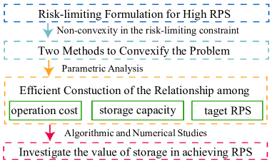
Figure 1: Paradigm to Investigate Value of Storage

Another well-investigated research direction is to design the storage control policies for arbitrage. For example, van de Ven et al. derive a threshold-based policy to minimize electricity cost for end-users facing price fluctuations in [5]. Wu et al. propose the optimal control policy for electricity storage against three-tier time of use pricing in [6]. Qin et al. propose an online algorithm to address two dimension of uncertainties in demand and price in [7].

Our work falls into a third group of research, which combines both perspectives. Chau et al. examine the control policy for storage with worst case performance guarantee in [8]. Different from their dynamic control approach, we seek to illuminate the value of storage from an algorithmic perspective. Debia et al. estimate the marginal value of energy storage in a power market with renewable energy and thermal generation in [9] with a focus on the two-period stylized model. In this paper, we consider a multi-stage decision making problem with risk-limiting constraints to highlight the cost induced by the high RPS. Such constraints are often non-convex, which further sophisticates the problem. We adopt the parametric functional approach [10] to address the non-convexity induced by risk-limiting constraints.

I-C Our Contributions

In seek of investigating the value of storage for RPS, our principal contributions can be summarized as follows:

• Risk-limiting Formulation: To evaluate the cost incurred by renewables, we use the notion of loss of load and include risk-limiting constraints in the decision making, which leads to a non-convex optimization problem.

• Problem Convexification: We introduce two methods to solve the risk-limiting constraints and convexify the decision making problem. Both methods provide the mapping between the reserved storage capacity and the limited risk.

• Analytical Characterization: We design an efficient algorithm to construct the function among electricity cost, storage capacity and the target RPS. This serves as the basis for our analytical understanding of the value of storage in achieving high RPS.

The rest of the paper is organized as follows. Section II introduces the system model and problem formulation. We tackle the challenges induced by the risk limiting constraints in Section III. After that, Section IV examines the value of storage from an algorithmic perspective. We share more insights through numerical studies in Section V. Finally, we deliver the concluding remarks and point out possible future directions in Section VI.

II System Model

We consider a stylized model where a microgrid operator installs certain renewables, as shown in Fig. 2. To meet demand $d_{t}$ (predicted as $\hat{d_{t}}$) at time $t$, the operator could purchase energy of $g_{t}$ directly from grid at real time price $p_{t}$; utilize the renewable energy of $r_{t}^{d}$; or conduct storage control.

Without the requirement of RPS, the operator would simply use storage for arbitrage against the real time price for more savings in electricity bills. However, in this model, we require the operator has to meet the target RPS of $\alpha$. This may result in the lost opportunity cost in arbitraging. Also, the system operator relies on the storage for reserving enough capacity to handle uncertainties in renewable generation.

To better model such uncertainties, at each time $t$, we denote the predicted and actual renewable generation by $\hat{r_{t}}$ and $r_{t}$, respectively. Facing such uncertainties and the strict RPS requirement, at each time $t$, we assume the system operator may either store energy of $a_{t}$ to storage, or discharge energy of $b_{t}$ to meet demand. In addition, the stored energy in storage may also come from the renewables, of amount $r_{t}^{s}$.

The microgrid system operator may seek to minimize the total electricity cost. Hence, we can formulate its decision making problem as follows:

$$\min\quad\ \sum\nolimits_{t=1}^{T}p_{t}(g_{t}+a_{t})$$ (1)

$$s.t.\quad g_{t}+b_{t}+r_{t}^{d}=\hat{d_{t}},\ \forall t,$$ (2)

$$\sum\nolimits_{t=1}^{T}(r_{t}^{d}+r_{t}^{s})=\alpha\sum\nolimits_{t=1}^{T}\hat{d_{t}},$$ (3)

$$x_{0}=x_{T}=0,\ x_{t}\geq 0,\ \forall t,$$ (4)

$$x_{t+1}=x_{t}+a_{t}+r_{t}^{s}-b_{t},\ t=1,...,T-1,$$ (5)

$$r_{t}^{s}+r_{t}^{d}\leq\hat{r_{t}},\ \forall t,$$ (6)

$$g_{t}\geq 0,\ a_{t}\geq 0,\ b_{t}\geq 0,\ r_{t}^{d}\geq 0,r_{t}^{s}\geq 0,\ \forall t,$$ (7)

$$x_{t}\leq B-\Delta,\ \forall t,$$ (8)

$$\Pr(\hat{d_{t}}-\hat{r_{t}}+\Delta\geq d_{t}-r_{t})\geq Q\%,\ \forall t$$ (9)

The decision variables are $g_{t}$,$a_{t}$,$b_{t}$,$r_{t}^{d}$ and $r_{t}^{s}$. We assume zero marginal cost of renewables. Hence, the cost function is only related to $g_{t}$ and $a_{t}$. Constraint (2) maintains the supply demand balance, and constraint (3) enforces the RPS requirement. The following two constraints are due to the evolving state-of-charge ($x_{t}$, at time $t$) in the storage system. Without loss of generality, we assume the decision horizon starts from mid-night when the price is often low. To achieve the maximal flexibility for the subsequent control, we require $x_{0}=0$. To eliminate pure arbitrage by the end of the decision making, we require $x_{T}=x_{0}$. Constraint (6) implies certain amount of renewable generation may be curtailed and constraint (7) indicates all the decision variables are non-negative. The final two constraints examine the value of storage. To satisfy the risk-limiting constraint $Q$, the operator may need to reserve certain storage capacity $\Delta$ as flexible resources, which in turn affects the feasible region of $x_{t}$’s.

Remark: We want to emphasize that this decision making problem is not limited to the microgrid scenario. For the grid level operation, we can directly replace the objective function with the total operation cost. Given the piece-wise linear structure of the operation cost, our subsequent analysis directly follows. We choose to use this microgrid scenario to better illustrate the notion-value of storage.

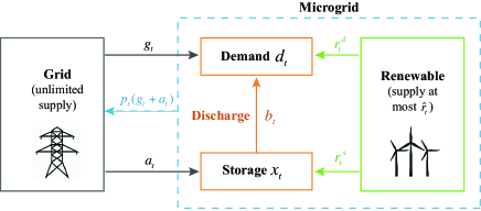
Figure 2: System Model

III Problem Convexification

The decision making problem is hard to solve due to the non-convexity in the risk-limiting constraint (9). Note that, the parameter $Q$ only affects the reserved capacity $\Delta$ in the optimization problem. Hence, we propose to first identify the suitable $\Delta$ before decision making.

Fact 1: The total cost $\sum_{t=1}^{T}p_{t}(g_{t}+a_{t})$ is non-decreasing in $\Delta$ in its feasible region.

This fact is based on the following observation: a larger $\Delta$ leads to a shrinked feasible region, and hence a no better total cost. This implies we can select the smallest $\Delta$ to satisfy the risk-limiting constraints:

$$\Delta(Q)\!=\!\min\{\delta\!:\!\Pr(\hat{d_{t}}\!-\!\hat{r_{t}}\!+\!\delta\geq d_{t}\!-\!r_{t})\geq Q\%,\ \forall t\}.$$ (10)

We choose a time-invariant $\Delta$ to sharp our understanding on the value of storage via limited parameters. In practice, one can definitely choose time varying $\Delta_{t}$ for more insights.

Unfortunately, even with this simplification, the risk-limiting constraint still display non-convex structure in general. One way to solve such non-convexity is to construct the mapping between $\Delta$ and $Q$ from the empirical prediction error distribution in demand and renewable generation. In practice, the demand prediction is rather accurate compared with that for renewable generation. Hence, in the subsequent analysis, we only consider the prediction error in the renewable generation and assume perfect demand prediction, i.e., $\hat{d_{t}}=d_{t},\forall t$.

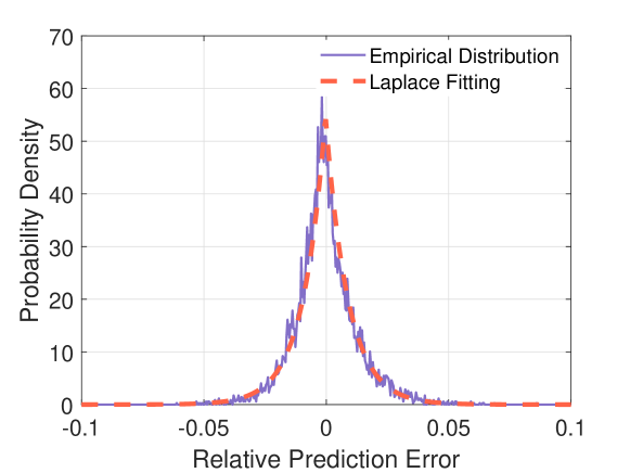
Figure 3: Laplace Fitting for Relative Prediction Error

By analyzing the European Network of Transmission System Operators for Electricity (ENTSO-E) data for wind power prediction [11], we observe that besides using the empirical probability distribution directly, we may also use Laplace distribution for approximation. This gives us an easier way to construct $\Delta(Q)$. Fig. 3 plots the fitted Laplace distribution and the relative error distribution, and Table I compares the functions $\Delta(Q)$ obtained from two approaches: $B_{e}$ is determined by the empirical error distribution, and $B_{L}$ is determined by the fitted Laplace distribution. For most cases, they are quite close. Either approach can help us convexify the optimization problem.

TABLE I: Reservation $\Delta$ for Different Risk-limiting Requirements

$Q\%$	0.7	0.8	0.9	0.93	0.96	0.99	0.998
$B_{e}$(MW)	54.11	86.17	138.3	162.3	202.4	322.6	438.9
$B_{L}$(MW)	50.10	86.17	146.3	174.3	222.4	342.7	483.0

IV Value of Storage: Algorithmic Understanding

We seek to understand three major parameters’ impacts on the minimal electricity cost: the storage capacity $B$, the risk-limiting parameter $Q$ (by the last section, it is equivalent to $\Delta$), and the RPS target $\alpha$.

We start our analytical study by raising the following question: given a RPS target $\alpha$, how will the minimal electricity cost change with respect to the storage capacity $B$? We can define a function $C_{\alpha}(\beta)$ as follows to answer this question:

$$\text{C}_{\alpha}(\beta)=\min\ \sum\nolimits_{t=1}^{T}p_{t}(g_{t}+a_{t})$$ (11)

$$s.t.\ x_{t}\leq\beta,$$ (12)

$$\alpha=\frac{\sum_{t=1}^{T}(r_{t}^{d}+r_{t}^{s})}{\sum_{t=1}^{T}\hat{d_{t}}},$$ (13)

$$\text{Constraints }(\ref{eq2}),(\ref{eq4})\text{-}(\ref{eq7}).$$ (14)

Using parametric LP analysis [12], we can show that the function $C_{\alpha}(\beta)$ has nice analytical properties.

Proposition 1: The $C_{\alpha}$ function is continuous, piecewise linear, convex and non-increasing in $\beta$.

We provide the detailed proof in Appendix. Here, we directly utilize the four properties to propose an efficient algorithm to construct the function $C_{\alpha}(\beta)$. We term the algorithm to construct $C_{\alpha}$ given $\alpha$ in range $[x,y]$ as Finding Breaking-points and Slopes FBS$(x,y)$, illustrated below.

Algorithm 1 FBS($x,y$)

0:  The RPS target $\alpha$.

1:  Compute $C_{\alpha}(x)$ and $C_{\alpha}(y)$ to get their Lagrangian multipliers $\lambda_{x}$ and $\lambda_{y}$ associated with (12), respectively;

2:  solve the system of equations below to obtain $z,c_{z}$;

$$\left\{\begin{array}[]{rcl}c_{z}-C_{\alpha}(x)=\lambda_{x}(z-x)\\ c_{z}-C_{\alpha}(y)=\lambda_{y}(z-y)\end{array}\right.$$ (17)

3:  if $c_{z}==C_{\alpha}(z)$ then

4:     $z$ is a breaking point, the slope in $[x,z]$ is $\lambda_{x}$ and the slope in $[z,y]$ is $\lambda_{y}$;

5:     Return;

6:  else

7:     Recursively construct FBS$(x,z)$ and FBS$(z,y)$;

8:  end if

Remark: The initial interval $[x_{0},y_{0}]$ for constructing $C_{\alpha}(\beta)$ can be determined with ease: $x_{0}$ can be selected as $0$ and $y_{0}$ can be any value that of decision maker’s interests. Such arbitrary selection won’t affect the algorithm efficiency as the time complexity of FBS is $O(n)$, where $n$ is the number of breaking points in the target function. Intuitively, in the worst case, $n$ could be exponentially large in the input size of the optimization problem. Fortunately, we can show that $n$ can be polynomially bounded by the input size [13] and in practice, $n$ is fairly small even for large system[10].

V Value of Storage: Numerical Studies

Besides the analytical properties, in this section, we want to share more insights behind the relationship function ($C_{\alpha}(\beta)$). We again use the ENTSO-E dataset with detailed data on annual wind generation and its forecast, annual demand and real-time price. The resolution is 1 hour. We plot some sample demand profiles and wind generation profiles in Fig. 4(a) and 4(b) respectively, with proper scaling. Clearly, the demand profiles display different patterns for weekdays and weekends, while wind power generation profiles highlight the stochastic nature. Fig. 5 visualizes the statistical features in the real time prices. From time to time, the ENSTO-E system witnesses negative prices, most likely due to strong wind. This also shows the possibility of achieving high RPS target in this system.

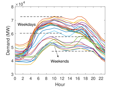
(a) Demand Pattern

(b) Wind Generation Pattern

Figure 4: Sample Patterns in ENTSO-E Data of 2018-2019.

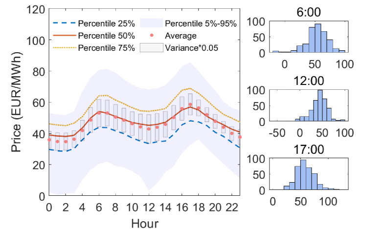
Figure 5: Statistical Features in Real Time Prices.

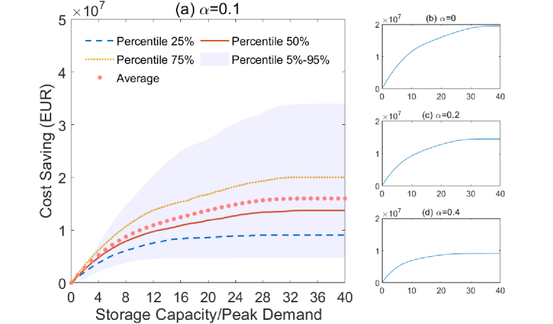
Figure 6: Cost Saving via Storage.

V-A Cost Savings From Storage

The most straightforward value of storage system to the operator is cost reduction. We define cost saving given RPS requirement of $\alpha$ by

$$\text{CS}(\beta|\alpha)\coloneqq C_{\alpha}(\beta)-C_{\alpha}(0).$$ (18)

Fig. 6 plots the cost saving evolves with increasing storage capacity. With different RPS targets ($\alpha=0,0.1,0.2,0.4$), we conduct the simulation for a year and use different percentiles to highlight the cost saving distributions. As shown in Fig. 6, even the percentile lines display certain piece-wise linear and convex structures, which verifies Proposition 1. Also, the marginal cost saving diminishes as storage capacity increases; a larger RPS requirement implies fewer cost saving: both coincides with our intuition, as dictated by Fact 1.

Figure 7: Lost Opportunity Cost for Arbitrage Caused by RPS.

Figure 8: Sample Storage Control Strategies

V-B Lost Opportunity Cost

We evaluate the value of storage by examining its lost opportunity cost, which is defined as follow:

$$\text{LOC}_{\text{RPS}}(\alpha|\beta)\coloneqq\text{CS}(\beta|0)-\text{CS}(\beta|\alpha).$$ (19)

Fig. 7 visualizes the function LOC${}_{\text{RPS}}(\alpha|\beta)$ given different storage capacities. One might believe that larger storage capacity implies larger flexibility region for decision making, and hence leads to a lower lost opportunity cost. However, such intuition is unfounded in Fig. 7. The reason is due to limited demand (more precisely, limited net demand) when RPS requirement is high, and storage cannot contribute too much in arbitrage. We highlight this counter-intuitive observation by randomly sampling a trace and plotting the optimal storage control with different parameters in Fig. 8. Due to limited net demand, even when $\alpha=0$, which means the operator can simply use the renewable generation as much as possible, by doubling the battery capacity, the battery control actions do not differ too much at most time slots. This illustrates the diminishing marginal value of storage system when its capacity is large enough.

On the other hand, we can define the lost opportunity cost from another perspective:

$$\text{LOC}_{\text{RL}}(\Delta(Q)|\beta)\coloneqq C_{\alpha}(\beta-\Delta(Q))-C_{\alpha}(\beta).$$ (20)

This implies the lost opportunity cost by reserving capacity for the risking limiting constraints. Fig. 9 visualizes this function, which displays a concave feature, and as the risk limiting constraints become tight, the cost increases dramatically. This observation further emphasizes the value of storage for a stable power system. In fact, we can use parametric analysis to show that $\text{LOC}_{\text{RL}}(\Delta|\beta)$ is piece-wise linear and concave in $\Delta$.

Remark: We want to conclude this section by pointing out additional properties of the three functions. All the three functions enjoy double optimality. The double optimality comes from the function $C_{\alpha}(\beta)$, which is the minimal electricity cost given a storage capacity of $\beta$. We can prove that given certain budget of $C_{\alpha}(\beta)$, to satisfy the risk limiting constraints and all other constraints, the minimal required storage capacity is exactly $\beta$. This can be proved by following the route in [10]. We omit the detailed proof due to page limit.

Figure 9: Lost Opportunity Cost of Reservation.

VI Conclusion

In this paper, we seek to understand the value of storage system to achieve high RPS. By convexifying the decision making problem, we use parametric analysis to understand the key parameters’ impacts on the decision making.

This work can be extended in many ways. For example, we haven’t considered the network constraints in the decision making, which will help understand how the transmission line congestion affects the value of storage system. The network constraints also raise interesting discussion on the trade-off between centralized storage system and geographically distributed storage system. Also, it will be interesting to consider time varying risk limiting constraints, which will include more temporal features in the decision making.

Appendix: Proof for Proposition 1

Proof: Continuity and piece-wise linearity are immediate results from Theorem 1.1-1.3 in [12]. The non-increasing property has been shown in Fact 1. Hence, it suffices to show the convexity of $C_{\alpha}(\beta)$.

Let $\beta_{1}$ and $\beta_{2}$ be arbitrary realization of storage capacity $B$, such that

$$\beta_{2}>\beta_{1}>0.$$ (21)

Denote the optimal solutions to $C_{\alpha}(\beta_{1})$ and $C_{\alpha}(\beta_{2})$ by $x_{1}$ and $x_{2}$, respectively. Hence,

$$x_{1} =(g_{1},a_{1},b_{1},r_{1}^{d},r_{1}^{s}),$$ (22)

$$x_{2} =(g_{2},a_{2},b_{2},r_{2}^{d},r_{2}^{s}).$$ (23)

To prove the convexity, it suffices to examine the property of $C_{\alpha}(\beta)$ at $\beta^{\prime}=\frac{1}{2}(\beta_{1}+\beta_{2})$. We can construct

$$x^{\prime}=\frac{1}{2}(x_{1}+x_{2}),$$ (24)

which is a feasible solution to $C_{\alpha}(\beta^{\prime})$. Due to the property of minimization problem, we have

$$C_{\alpha}\left(\frac{\beta_{1}+\beta_{2}}{2}\right) =C_{\alpha}(\beta^{\prime})\leq\sum_{t=1}^{T}p_{t}(g_{t}^{\prime}+a_{t}^{\prime})$$ (25)

$$=\frac{1}{2}C_{\alpha}(\beta_{1})+\frac{1}{2}C_{\alpha}(\beta_{2}).$$

The convexity immediately follows. $\hfill\blacksquare$

References

- [1] G. Barbose, R. Wiser, J. Heeter, T. Mai, L. Bird, M. Bolinger, A. Carpenter, G. Heath, D. Keyser, J. Macknick et al., “A retrospective analysis of benefits and impacts of us renewable portfolio standards,” Energy Policy, vol. 96, pp. 645–660, 2016.
- [2] H. Zhao, Q. Wu, S. Hu, H. Xu, and C. N. Rasmussen, “Review of energy storage system for wind power integration support,” Applied energy, vol. 137, pp. 545–553, 2015.
- [3] F. J. De Sisternes, J. D. Jenkins, and A. Botterud, “The value of energy storage in decarbonizing the electricity sector,” Applied Energy, vol. 175, pp. 368–379, 2016.
- [4] E. Bitar, P. Khargonekar, and K. Poolla, “On the marginal value of electricity storage,” Systems & Control Letters, vol. 123, pp. 151–159, 2019.
- [5] P. M. van de Ven, N. Hegde, L. Massoulié, and T. Salonidis, “Optimal control of end-user energy storage,” IEEE Transactions on Smart Grid, vol. 4, no. 2, pp. 789–797, 2013.
- [6] C. Wu and Y. Yu, “Optimal control for electricity storage against three-tier tou pricing,” in 2018 Asia-Pacific Signal and Information Processing Association Annual Summit and Conference (APSIPA ASC). IEEE, 2018, pp. 737–741.
- [7] J. Qin, Y. Chow, J. Yang, and R. Rajagopal, “Online modified greedy algorithm for storage control under uncertainty,” IEEE Transactions on Power Systems, vol. 31, no. 3, pp. 1729–1743, 2015.
- [8] C.-K. Chau, G. Zhang, and M. Chen, “Cost minimizing online algorithms for energy storage management with worst-case guarantee,” IEEE Transactions on Smart Grid, vol. 7, no. 6, pp. 2691–2702, 2016.
- [9] S. Debia, P.-O. Pineau, and A. S. Siddiqui, “Strategic use of storage: The impact of carbon policy, resource availability, and technology efficiency on a renewable-thermal power system,” Energy Economics, vol. 80, pp. 100–122, 2019.
- [10] C. Wu, G. Hug, and S. Kar, “Risk-limiting economic dispatch for electricity markets with flexible ramping products,” IEEE Transactions on Power Systems, vol. 31, no. 3, pp. 1990–2003, 2015.
- [11] E. N. of Transmission System Operators for Electricity, “Central collection and publication of electricity generation, transportation and consumption data and information for the pan-european market.” https://transparency.entsoe.eu/.
- [12] A. Holder, “Parametric lp analysis,” Wiley Encyclopedia of Operations Research and Management Science, 2010.
- [13] T. K. Dey, “Improved bounds on planar k-sets and k-levels,” in Proceedings 38th Annual Symposium on Foundations of Computer Science. IEEE, 1997, pp. 156–161.