Rademacher complexity and spin glasses:
A link between the replica and statistical theories of learning
CNRS & CEA & Université Paris-Saclay, Saclay, France
Laboratoire de Physique Statistique
CNRS & Sorbonnes Universités &
École Normale Supérieure, PSL University, Paris, France
)
Abstract
Statistical learning theory provides bounds of the generalization gap, using in particular the Vapnik-Chervonenkis dimension and the Rademacher complexity. An alternative approach, mainly studied in the statistical physics literature, is the study of generalization in simple synthetic-data models. Here we discuss the connections between these approaches and focus on the link between the Rademacher complexity in statistical learning and the theories of generalization for typical-case synthetic models from statistical physics, involving quantities known as Gardner capacity and ground state energy. We show that in these models the Rademacher complexity is closely related to the ground state energy computed by replica theories. Using this connection, one may reinterpret many results of the literature as rigorous Rademacher bounds in a variety of models in the high-dimensional statistics limit. Somewhat surprisingly, we also show that statistical learning theory provides predictions for the behavior of the ground-state energies in some full replica symmetry breaking models.
1 Introduction
Empirical risk minimization is the workhorse of most of modern supervised machine learning successes. Consider for instance a data-set of examples assumed to be drawn from a distribution , with labels used for a binary classification task. We consider an estimator that belongs to a hypothesis class , for instance a neural network or a linear function, with respective weights or parameters w. The latter are typically computed by minimizing the empirical risk
over w, where denotes a loss function, e.g. the mean-squared-loss . The main theoretical issue of statistical learning theory concerns the performance of the estimator obtained by such a minimization on yet unseen data, namely the generalization problem. In fact, what we really hope to minimize is the population risk, defined as
Since we are optimizing the empirical risk instead, the difference between the two might be arbitrarily large. Bounding this difference between empirical and population risks is therefore a major problem of statistical learning theories.
In a large part of the literature, statistical learning analysis (see e.g. [1, 2, 3]) relies on the Vapnik-Chervonenkis (VC) analysis and on the so-called Rademacher complexity. The latter is a measure of the complexity of , the hypothesis class spanned by , to bound , the generalization gap. A gem within the literature is the Uniform Convergence result which states the following: if the Rademacher complexity or the VC dimension is finite, then for a large enough number of samples the generalization gap will vanish uniformly over all possible values of parameters w. Informally, uniform convergence tells us that with high probability, for any weights value w, the generalization gap satisfies
| (1) |
where denotes the Vapnik-Chervonenkis dimension of the hypothesis class . Tighter bounds can be obtained using the Rademacher complexity. These bounds, although useful, do not seem to fully explain the success of current deep-learning architectures ([4]).
Over the last four decades, a different vision of generalization — based on the analysis of typical case problems with synthetic data created from simple generative models — was developed to a large extent in the statistical physics literature (see e.g. [5, 6, 7, 8] for a review). The link with the VC dimension was discussed in many of these works, notably via its connection with its twin from statistical physics, the Gardner capacity ([9]). In particular, one can show that the VC capacity is always larger than half of the Gardner one ([8]). We shall review this discussion later on in this paper. However, to the best of our knowledge the Rademacher complexity was absent from these considerations. This omission is unfortunate: not only does the Rademacher complexity give tighter bounds than the VC dimension, it also intrinsically connects with a quantity that physicists are familiar with and have been computing from the very beginning of their studies, namely the average ground-state energy.
The goal of the present paper is to bridge this gap and unveil the deep link between ground-state energy and Rademacher complexity, and how this connection is valuable to both parties. The paper is organized as follows: After giving proper definitions of common generalization bounds in sec. 2, we detail calculations of Rademacher complexities for simple function classes in sec. 3. These sections serve as an introduction to the readers not familiar with these notions. The subsequent sections 4 and 5 provide the original content of the paper.
Here we summarize the main contributions of this paper:
-
•
We point out the one-to-one connections between the Rademacher complexity in statistical learning, and the ground-state energies and Gardner capacity from statistical physics.
-
•
We show how the heuristic replica method from statistical physics can be used to compute the Rademacher complexity in the high-dimensional statistics limit and reinterpret classical results of the statistical physics literature as Rademacher bounds in the case of perceptron and committee machine models with i.i.d data.
-
•
We contrast these results with the generalization in the teacher-student scenario, illustrating the worst-case nature of the Rademacher bound that fails to capture the typical-case behavior.
-
•
We finally show en passant, that learning theory also bears consequences for the spin glass physics and the related replica symmetry breaking scheme by showing it implies strong constraint on the ground-state energy of some spin glass models.
2 A primer on Rademacher complexity
The bound of the generalization gap involving the VC dimension is specific to binary classification, and does not depend on the data distribution. While this is a strong property, the Rademacher approach does depend on data distribution and allows for tighter bounds. Moreover, it generalizes to multi-class classification and regression problems. We recall the definition of the Rademacher complexity:
Definition 2.1.
Let be any function in the hypothesis class , and let be drawn uniformly at random. The empirical Rademacher complexity is defined as
| (2) |
and depends on the sample examples . The Rademacher complexity is defined as the population average
| (3) |
In this paper, we shall focus on binary classification and consider the corresponding loss function that counts the number of misclassified samples. We will be therefore interested in a hypothesis class . Defining the training and generalization errors for any function by
| (4) |
the Rademacher complexity provides a generalization error bound as expressed by the following theorem, and many of its variants (see e.g. [1, 2, 3, 10]):
Theorem 2.2 (Uniform convergence bound - Binary classification).
Fix a distribution and let . Let be drawn i.i.d from . Then with probability at least (over the draw of ),
| (5) |
Thus, the Rademacher complexity is a uniform bound of the generalization gap. In the high-dimensional limit, i.e when both and go to infinity, that we will consider in the remaining of the paper we shall see that we can discard the dependent term and that only the first term will remain finite.
Note that this theorem can be used to recover the classical result (1). Indeed it can be shown ([11, 12, 13]) that the Rademacher complexity can be bounded by the VC dimension so that for some constant value ,
| (6) |
We remind the reader that the VC dimension is the size of the set that can be fully shattered by the hypothesis class . Informally, if then for all set of data points, there exists an assignment of labels that cannot be fully fitted by the function class ([2]).
3 Synthetic models in the high-dimensional statistics limit
In this section, we consider data generated by a simple generative model. We suppose that each vector of the input data points has been generated i.i.d from a factorized, e.g. Gaussian, distribution, that is . In the following, we will focus on this simple data distribution, but sec. 5.5 presents a generalization to rotationally invariant data matrices with arbitrary spectrum. The main interest of such settings is to use the analysis of typical case problems with synthetic data created from simple generative models as means of getting additional insight on real world applications where data are not worst case ([5, 6, 7, 8, 14]). In particular, we shall be interested in the high-dimensional statistics limit when , with . In this paper, the aim is to compute exactly (rather than merely bounding) and asymptotically the Rademacher complexity for such problems.
3.1 Linear model
As the simplest example, we first tackle the computation of the Rademacher complexity for a simple function class containing all linear models with weights ,
| (7) |
From eq. (3), computing the empirical Rademacher complexity amounts to finding the vector that maximizes the scalar product between y (that replaces the variable ) and . It is thus sufficient to take and the empirical Rademacher complexity (3) thus reads
| (8) |
having i.i.d entries, we can apply the central limit theorem, which enforces , hence . Assuming that weights are restricted to lie on the sphere of radius , we set and finally obtain
| (9) |
where recall . The above result for the simple linear function hypothesis class allows to grasp the meaning of the Rademacher complexity: At fixed input dimension , it decreases with the number of samples as , closing the generalization gap in the infinite limit. Illustrating the bias-variance trade-off, we also see that increasing the radius of the weights expands the function complexity (and might help for fitting the data-set), but unfortunately leads to a looser generalization bound.
Note also that the fact that the Rademacher complexity is shows that it remains finite in the high-dimensional statistics limit. In this case, we see indeed that we can disregard the term that goes to zero as in eq. (5).
3.2 Perceptron model
The scaling of the Rademacher complexity inverse as in the high-dimensional statistics limit is actually not restricted to the linear model but appears to be a universal property, at least at large enough . To see this we now focus on a different hypothesis class: the perceptron, denoted . This class contains linear classifiers which output binary variables, and will fit much better labels in the binary classification task. The class is defined as
| (10) |
Let us consider a sample i.i.d matrix with .
Theorem 3.1.
For the perceptron model class eq. (10) with random i.i.d. input data in the high-dimensional limit, .
The proof is given in Appendix A. In a nutshell, it uses the fact that Rademacher complexity is upper-bounded by the VC dimension divided by , and lower-bounded by one particular example of its function class, when the weights are chosen according to Hebb’s rule ([15]), which also gives a behavior scaling as .
Heuristically, this result generalizes as well to a two-layer neural network with hidden neurons. Indeed, the two-layer function class contains, as a particular case, the single layer one, so the lower bounds goes through. The upper bound is however harder to control rigorously. Since neural networks have a finite VC dimension, the Rademacher complexity is again lower-bounded by ; However, we do not know of any theorem that would ensure that the VC dimension is bounded by ([16]). Nevertheless, anticipating on the statistical physics approach, we indeed expect from the concentration (self-averaging) properties of the ground-state energy ([17]) in the high-dimensional limit that it will yield a Rademacher complexity that is a function of only at fixed . From this argument, we expect that the dependence of the Rademacher complexity to be very generic in the high-dimensional limit.
4 The statistical physics approach
4.1 Average case problems: Statistical physics of learning
As anticipated in the previous chapter, the approach inspired by statistical physics to understand neural networks considers a set of data points coming from known distributions. Again, for the purpose of this presentation we focus on a simple example, where with . Sec. 5.5 is devoted to a generalization to random input data corresponding to random matrices with arbitrary singular value density.
Consider a function class, for instance we can again use the perceptron one : ; a typical question in the literature was to compute how many misclassified examples can be obtained for a given rule used to generate the labels ([8]). Given samples , in order to count the number of wrongly classified training samples, we define the Hamiltonian, or energy function [18]:
| (11) |
A classical problem in statistical physics is to compute the random capacity also called Gardner capacity ([19]): given examples and labels randomly chosen between , it consists in finding how many samples can be correctly classified.
It turns out there exists a deep connection between the Gardner capacity and the VC dimension, as their common aim is to measure the maximum number of points such that there exists a function in the hypothesis class being able to fit the data set. In particular, using Sauer’s lemma ([20]) in the large size limit , keeping and , it is possible to show that the Gardner capacity provides a lower-bound of the VC dimension ([8]):
| (12) |
To illustrate this inequality, let us consider again the perceptron classifier hypothesis class for which the above inequality is saturated. In fact, the VC dimension is in this case (linear classification with binary outputs) simply . Hence on one hand and on the other hand the Gardner capacity amounts to ([21, 19]).
4.2 The Rademacher complexity and the ground-state energy
As we shall see now, computing the Rademacher complexity for random input data can be directly reduced to a more natural object in the physics literature: the ground-state energy. Defining the Gibbs measure at inverse temperature , that weighs configurations with their respective cost, as
| (13) |
we observe that averaging the Hamiltonian in eq. (11) over and the Gibbs measure at temperature for any function provides
| (14) |
where . Taking the zero temperature limit, i.e. , in the above equation, we finally obtain the ground-state energy , a quantity commonly used in physics. Interestingly, we recognize the definition of the Rademacher complexity
| (15) |
where random labels y play the role of the Rademacher variable in (3). The above equation shows a simple correspondence between the ground-state energy of the perceptron model and the Rademacher complexity of the corresponding hypothesis class, and shall bring insights from both the machine learning and statistical physics communities. Consequently, as we shall see, this connection means that the Rademacher complexity can be computed (rather than bounded) for many models using the replica method from statistical physics. As far as we are aware, this basic connection between the ground state energy and Rademacher complexity was not previously stated in literature.
4.3 An intuitive understanding on the Rademacher bounds on generalization
At this point, the Rademacher complexity becomes a more familiar object to the physics-minded reader. However, could we understand more intuitively why the Rademacher complexity, or equivalently the ground-state energy, is involved in the generalization gap bound? Let us present an intuitive hand-waving explanation. Consider the fraction of mistakes performed by a classifier on unknown samples, namely the generalization error , and on the training set, the training error . The worst case scenario that could occur is trying to fit while there exists no underlying rule, meaning that labels are purely random uncorrelated from input. The estimator will purely overfit and its generalization error will remain constant to in any case. This leads to the following heuristic generalization bound:
| (16) |
Note that this heuristic reasoning does not give the exact Rademacher generalization bound. In fact, the actual stronger and uniform (over all possible ) bound does not have a factor , and surely cannot be fully captured by the simple above argument. Nevertheless, this argument reflects the crux of the Rademacher bound: it provides a very pessimistic bound by assuming the worst possible scenario: i.e. fitting data and trying to make predictions while the labels are random. Of course, in real data problems the rule is not random; it is then no surprise that the Rademacher bound is not tight ([4]). Indeed, real problems labels are not randomly correlated with the inputs.
5 Consequences and bounds for simple models
In this section, we illustrate our previous arguments and the connection between the spin glass approach and the Rademacher complexity still for the case of Gaussian i.i.d input data matrix in the high-dimensional limit when .
5.1 Ground state energies of the perceptron
For a number of samples smaller than the Gardner capacity , it is by definition possible to fit all random labels y. Accordingly, the number of misclassified examples is zero and the ground state energy . This means that the Rademacher complexity is asymptotically equal to for . However above the Gardner capacity , the estimator cannot perfectly fit the random labels and will misclassify some of them, equivalently . From the arguments given in sec. 3, we thus expect
| (17) | ||||
This relation is already non-trivial, as it yields a link between the Gardner capacity and the Rademacher complexity. Using the replica method from spin glass analysis, and the mapping with ground state energies (15), we shall now see how one can go beyond these simple arguments, and compute the actual precise asymptotic value of the Rademacher complexity.
5.2 Computing the ground-state energy with the replica method
Knowing that statistical physics literature focused mainly on the Gardner capacity, the connection between the ground-state energy and the Rademacher complexity suggests that it would be worth looking at these old results in a new light. In fact, the replica method allows for an exact computation of the Rademacher complexity for random input data in the large size limit. In the following, we handle computations by focusing on a simple generalization of the linear functions hypothesis class. Fix any activation function , we define the following hypothesis class
| (18) |
Starting with the posterior distribution
| (19) |
we introduced the partition function associated to the Hamiltonian eq. (11) at inverse temperature
| (20) |
In the large size limit , the posterior distribution becomes highly peaked in particular regions of parameters. In physics we are interested in these dominant regions and focus on the free energy at inverse temperature defined as
| (21) |
However, as we are interested in computing quantities in the typical case, we want to average over all potential training sets and compute instead the averaged free energy
| (22) |
Computing directly this average rigorously is difficult, hence we will carry out the computation using the so-called replica method, starting by writing the replica trick
| (23) |
which replaces the expectation of by the moments of , which are easier to compute. For the non-familiar reader, it is instructive to remark that we introduced the partition function of non-interacting copies, also called replicas, of the initial system with partition function . Assuming there exists an analytical continuation and that we can revert both limits, we can finally take the limit
| (24) |
We give some details on the replica computation in Appendix B.1, and we also refer the reader to the relevant literature in physics ([18, 26, 8, 27, 14]) and in mathematics ([17, 23, 28, 29, 30]). The computation of the high-dimensional posterior and corresponding free energy (24) reduces to an optimization problem over two symmetric matrices which describe the correlations (induced by the average) between the aforementioned fictive replicas. In particular the off-diagonal terms of the matrix measure the overlaps between the different replicas, while the diagonal term is fixed to . We can therefore derive the free energies corresponding to a hierarchy of approximate ansatz on these matrices and , named replica symmetric (RS), one-step replica-symmetry breaking (1RSB), two-step replica-symmetry breaking (2RSB)…The different ansatz describe different solution space structures and we refer the interested reader to Appendix B.1.2 and B.1.2 for more details. While in some problems the RS or the 1RSB ansatz are sufficient, in others only the infinite step solution (full-RSB) gives the exact ansatz ([31, 17, 23]), although the 1RSB approach is usually an accurate approximation.
Computing the ground state energy consists in taking the zero temperature limit above the capacity in the replica free energy ; where denote respectively the energy and entropy contributions. The simplest form of the replica computation is known as Replica Symmetric (RS) and the next simplest is one-step Replica-Symmetry Breaking (1RSB) which plugged in eq. (24) leads to expressions [32, 33, 34]
| (25) |
where denote the overlap order parameters and the auxiliary functions
| (26) |
where denote two i.i.d normal random variables, and the distribution of the random labels. We introduced a temperature-dependant constraint function where the generic cost function reads in our case . Above expressions are valid for any generic weight distribution and non-linearity . The detailed computation can be found in Appendix B.1, in particular eq. (53) and eq. (65). Then the general method to find the ground state energy is to take the zero temperature limit
| (27) |
while handling carefully the scaling of the optimized order parameters in this limit.
Spherical perceptron
The most commonly studied model ([9, 36, 19, 9]) with continuous weights is the spherical model with such that . The spherical constraint allows to have a well-defined model which excludes diverging or vanishing weights. In this case, the Gardner capacity is rigorously known to be equal to ([21]).
We computed the RS, 1RSB and 2RSB free energies ([32, 33, 34], see details in Appendix B.1.5.). Taking the zero temperature limit with and finite in the RS ansatz and keeping and finite in the 1RSB case, leads to the following expressions of the ground states energies:
| (28) | ||||
| (29) | ||||
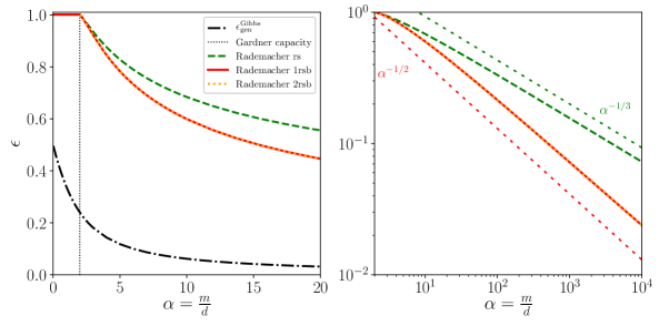
where the cost function . The details of the derivation via the replica method and the expression for the 2RSB ansatz are given in Appendix B.1.5. The results for Rademacher variable and with are depicted in Fig. 1.
Interestingly, the bounds on the Rademacher complexity also induce consequences on spin glass physics. Indeed as the large scaling of the ground state energy is not generally prescribed, the fact that the Rademacher complexity scales as for large values of — namely there exists a constant such that — implies that the ground state energy behaves for large as
| (30) |
We first notice that the replica symmetric (RS) solution complexity fails to deliver the correct scaling as sketched in Fig. 1, so the scaling in eq. (30) must not be entirely trivial. On the other hand, the 1RSB and 2RSB solutions we used (which are expected to be numerically very close to the harder to evaluate full-RSB one), seems to yield the correct scaling (see Fig. 1). It is rather striking that the statistical learning connection allows to predict, through eq. (30), the scaling of the energy in the large regime, that is only satisfied with replica-symmetry breaking ansatz. This yields an open question for replica theory: in practice, can one compute exactly the value of the constant ? Given the full-RSB solution is notoriously hard to evaluate, this might be an issue worth investigating in mathematical physics.
Binary perceptron
Another common choice for the weights distribution is the binary prior
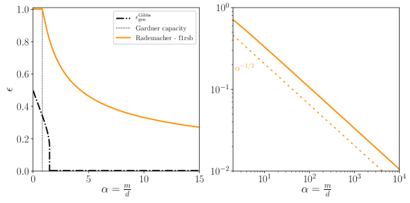
studied e.g. in [22]. In this case, the Gardner capacity is predicted to be , a prediction which, remarkably, is still not entirely rigorously proven, but see [24, 25].
To see this, we use eq. (25). In the binary perceptron, the landscape of the model is said to be frozen 1RSB (f1RSB), i.e. clustered in point-like dominant solutions, and the RS and 1RSB free energies are the same (even though their entropies are different) . In this case computing the ground state can be tackled via finding the effective temperature such that the , that can be plugged back to find the ground state energy . Again, we note that even though the 1RSB ansatz is unstable and should be replaced by a more complex (and ultimately full-RSB) solution, it already gives the good scaling , and satisfies the scaling eq. (30) for large , as in the case of the spherical model, see Fig. 2.
5.3 Teacher-student scenario versus worst case Rademacher
The Rademacher bounds are really interesting as they depend only on the data distribution, and are valid for any rule used to generate the labels, no matter how complicated. In this sense, it is a worst-case scenario on the rule that prescribes labels to data. A different approach, again pioneered in statistical physics [19], is to focus on the behavior for a given rule, called the teacher rule. Given the Rademacher bounds tackle the worst case with respect to that rule, it is interesting to consider the generalization error one actually gets for the best case, i.e. fitting the labels according to the same teacher rule.. This is the so-called teacher-student approach. In the wake of the need to understand the effectiveness of neural networks, and the limitations of the classical approaches, it is of interest to revisit the results that have emerged thanks to the physics perspective.
We shall thus assume that the actual labels are given by the rule
| (31) |
with , the teacher weights that can be taken as Rademacher variables, or Gaussian ones. Now that labels are generated by feeding i.i.d random samples to a neural network architecture (the teacher) and are then presented to another neural network (the student) that is trained using this data, it is interesting to compare the worst case Rademacher bound with the actual generalization error of this student on such synthetic data.
We now consider the error of a typical solution w from the posterior distribution (this is often called the Gibbs rule) for the student. Given the rule is outputting variables, this yields
| (32) |
where . Computing the replica symmetric overlap can be done within the statistical mechanics approach ([5, 6, 7, 8]) and can be rigourously done as well ([35]). Notice that this error is equal to the Bayes optimal error for the quadratic loss (see as well [35]).
The two optimistic (teacher-student) and pessimistic (Rademacher) errors can be seen in Fig. 1 for spherical and in Fig. 2 for binary weights. In this case, since a perfect fit is always possible, the training error is zero and the Rademacher complexity is itself the bound on the generalization error. These two figures show how different the worst and teacher-student case can be in practice, and demonstrate that one should perhaps not be surprised by the fact that the empirical Rademacher complexity does not always give the correct answer [4], as after all it deals only with worst case scenarios.
5.4 Committee machine with Gaussian weights
Given the large gap between the Rademacher bound and the teacher-student setting, we can ask wheather we can find a case where the Rademacher bound is void in the sense that the Rademacher complexity is yet generalization is good for the teacher-student setting? This can be done by moving to two-layer networks. Consider a simple version of this function class, namely the committee machine [8]. It is a two-layer network where the second layer has been fixed, such that only weights of the first layer are learnt. The function class for a committee machine with hidden units is defined by
| (33) |
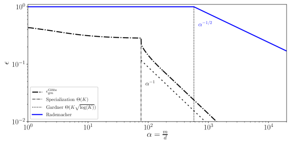
Instead of computing the Rademacher complexity with the replica method, it is sufficient for the purpose of this section to understand its rough behavior. As discussed in sec. 5.1, this requires knowing the Gardner capacity. A generic bound by [37] states that it is upper bounded by . Additionally, the Gardner capacity has been computed by the replica method in [38, 39, 40] who obtained that . We thus expect that
| (34) | ||||
To compare with the teacher-student case, when the labels are produced by a teacher committee machine as
| (35) |
the error of the Gibbs algorithm reads
| (36) |
where, again , has been computed in a series of papers in statistical physics [26, 41], and using the Guerra interpolation method in [42]. Interestingly, in this case, one can get an error that decays as as soon as . One thus observes a huge gap between the Rademacher bound that scales as and the actual generalization error for large sample size. This large gap further illustrates the considerable difference in behavior one can get between the worst case and teacher-student case analysis, see Fig. 3.
5.5 Extension to rotationally invariant matrices
The previous computation for i.i.d data matrix X can be generalized to rotationally invariant (RI) random matrices with rotation matrices , independently sampled from the Haar measure, and a diagonal matrix of singular values. Computation for this kind of matrices can be handled again using the replica method ([43, 44, 45]) and leads to RS and 1RSB free energies
| (37) |
where each term is properly defined in Appendix B.2. Note that taking a random Gaussian i.i.d matrix, the eigenvalue density follows the Marchenko-Pastur distribution and (37) matches free energies eq. (53), (65), and ground states energies eq. (28) in the spherical case. The ground state energy (and therefore the Rademacher complexity) can be again computed as in the i.i.d case, taking the zero temperature limit
| (38) |
keeping in particular and finite in the limits .
6 Conclusion
In this paper, we discussed the deep connection between the Rademacher complexity and some of the classical quantities studied in the statistical physics literature on neural networks, namely the Gardner capacity, the ground-state energy of the random perceptron model, and the generalization error in the teacher-student model. We believe it is rather interesting to draw the link with approaches inspired by statistical physics, and compare its findings with the worst-case results. In the wake of the need to understand the effectiveness of neural networks and also the limitations of the classical approaches, it is of interest to revisit the results that have emerged thanks to the physics perspective. This direction is currently experiencing a strong revival, see e.g. [46, 47, 48, 49]. The connection discussed in the paper opens the way to a unified presentation of these often contrasted approaches, and we hope this paper will help bridging the gap between researchers in traditional statistics and in statistical physics. There are many possible follow-ups, the more natural one being the computation of Rademacher complexities from statistical physics methods for more complicated and realistic models of data, starting for instance with correlated matrices discussed in section 5.5.
7 Acknowledgements
This work is supported by the ERC under the European Union’s Horizon 2020 Research and Innovation Program 714608-SMiLe, as well as by the French Agence Nationale de la Recherche under grant ANR-17-CE23-0023-01 PAIL and from the Chaire CFM-ENS. We thank Henry Pfister for insightful and clarifying discussions that inspired partly this work. We would also like to thank the Kavli Institute for Theoretical Physics (KITP) for welcoming us during part of this research, with the support of the National Science Foundation under Grant No. NSF PHY-1748958.
References
- [1] Peter L Bartlett and Shahar Mendelson. Rademacher and Gaussian complexities: Risk bounds and structural results. Journal of Machine Learning Research, 3(Nov):463–482, 2002.
- [2] Vladimir Vapnik. The nature of statistical learning theory. Springer science & business media, 2013.
- [3] Shai Shalev-Shwartz and Shai Ben-David. Understanding machine learning: From theory to algorithms. Cambridge university press, 2014.
- [4] Chiyuan Zhang, Samy Bengio, Moritz Hardt, Benjamin Recht, and Oriol Vinyals. Understanding deep learning requires rethinking generalization. ICLR 2017, preprint arXiv:1611.03530, 2016.
- [5] H Seung, H Sompolinsky, and N Tishby. Statistical mechanics of learning from examples. Physical Review A, 45(8):6056–6091, 1992.
- [6] Timothy L H Watkin and Albrecht Rau. The statistical mechanics of learning a rule. Review of Modern Physics, 65:499–556, 1993.
- [7] Manfred Opper. Statistical mechanics of learning: Generalization. The Handbook of Brain Theory and Neural Networks,, pages 922–925, 1995.
- [8] Andreas Engel and Christian Van den Broeck. Statistical mechanics of learning. Cambridge University Press, 2001.
- [9] Elizabeth Gardner and Bernard Derrida. Optimal storage properties of neural network models. Journal of Physics A: Mathematical and general, 21(1):271, 1988.
- [10] Mehryar Mohri, Afshin Rostamizadeh, and Ameet Talwalkar. Foundations of Machine Learning. The MIT Press, 2nd edition, 2018.
- [11] Pascal Massart. Some applications of concentration inequalities to statistics. In Annales de la Faculté des sciences de Toulouse: Mathématiques, volume 9, pages 245–303, 2000.
- [12] Michel Ledoux and Michel Talagrand. Probability in Banach Spaces: isoperimetry and processes. Springer Science & Business Media, 2013.
- [13] Richard M Dudley. The sizes of compact subsets of Hilbert space and continuity of Gaussian processes. Journal of Functional Analysis, 1(3):290–330, 1967.
- [14] Lenka Zdeborová and Florent Krzakala. Statistical physics of inference: thresholds and algorithms. Advances in Physics, 65(5):453–552, 2016.
- [15] Donald Olding Hebb. The organization of behavior: a neuropsychological theory. Science Editions, 1962.
- [16] Peter L Bartlett and Wolfgang Maass. Vapnik-chervonenkis dimension of neural nets. The handbook of brain theory and neural networks, pages 1188–1192, 2003.
- [17] Michel Talagrand. Spin glasses: a challenge for mathematicians: cavity and mean field models, volume 46. Springer Science & Business Media, 2003.
- [18] M. Mézard, G. Parisi, and M. A. Virasoro. SK model: The replica solution without replicas. Epl, 1(2):77–82, 1986.
- [19] E. Gardner and B. Derrida. Three unfinished works on the optimal storage capacity of networks. Journal of Physics A: Mathematical and General, 22(12):1983–1994, 1989.
- [20] N Sauer. On the density of families of sets. Journal of Combinatorial Theory, Series A, 13(1):145 – 147, 1972.
- [21] T. M. Cover. Geometrical and statistical properties of systems of linear inequalities with applications in pattern recognition. IEEE Transactions on Electronic Computers, EC-14(3):326–334, June 1965.
- [22] W Krauth and M Mezard. Storage capacity of memory networks with binary coupling. J. Phys (France), 50:3057–3066, 1989.
- [23] Michel Talagrand. The Parisi formula. Annals of mathematics, pages 221–263, 2006.
- [24] Jian Ding and Nike Sun. Capacity lower bound for the Ising perceptron. In Proceedings of the 51st Annual ACM SIGACT Symposium on Theory of Computing, pages 816–827. ACM, 2019.
- [25] Benjamin Aubin, Will Perkins, and Lenka Zdeborová. Storage capacity in symmetric binary perceptrons. Journal of Physics A: Mathematical and Theoretical, 52(29):294003, 2019.
- [26] John Hertz and Holm Schwarze. Generalization in large committee machines. Physica A: Statistical Mechanics and its Applications, 200(1-4):563–569, 1993.
- [27] Marc Mezard and Andrea Montanari. Information, physics, and computation. Oxford University Press, 2009.
- [28] Erwin Bolthausen and Anton Bovier. Spin glasses. Springer, 2007.
- [29] Dmitry Panchenko and Michel Talagrand. Bounds for diluted mean-fields spin glass models. Probability Theory and Related Fields, 130(3):319–336, 2004.
- [30] Dmitry Panchenko et al. Free energy in the potts spin glass. The Annals of Probability, 46(2):829–864, 2018.
- [31] Marc Mézard. The space of interactions in neural networks: Gardner’s computation with the cavity method. Journal of Physics A: Mathematical and General, 22(12):2181–2190, 1989.
- [32] P. Majer, A. Engel, and A. Zippelius. Perceptrons above saturation. Journal of Physics A: Mathematical and General, 26(24):7405–7416, 1993.
- [33] R Erichsen and W K Thuemann. Optimal storage of a neural network model: a replica symmetry-breaking solution. Journal of Physics A: Mathematical and General, 26(2):L61–L68, jan 1993.
- [34] W. Whyte and D. Sherrington. Replica-symmetry breaking in perceptrons. Journal of Physics A: Mathematical and General, 29(12):3063–3073, 1996.
- [35] Jean Barbier, Florent Krzakala, Nicolas Macris, Léo Miolane, and Lenka Zdeborová. Optimal errors and phase transitions in high-dimensional generalized linear models. Proceedings of the National Academy of Sciences, 116(12):5451–5460, 2019.
- [36] E Gardner. The space of interations in neural network models. J. Phys. A, 21:257, 1988.
- [37] G. J. Mitchison and R. M. Durbin. Bounds on the learning capacity of some multi-layer networks. Biological Cybernetics, 60(5):345–365, Mar 1989.
- [38] Rémi Monasson and Riccardo Zecchina. Weight space structure and internal representations: A direct approach to learning and generalization in multilayer neural networks. Physical Review Letters, 75(12):2432–2435, Sep 1995.
- [39] R Urbanczik. Storage capacity of the fully-connected committee machine. Journal of Physics A: Mathematical and General, 30(11):L387, 1997.
- [40] Yuansheng Xiong, Chulan Kwon, and Jong-Hoon Oh. The storage capacity of a fully-connected committee machine. In Advances in Neural Information Processing Systems, pages 378–384, 1998.
- [41] Henry Schwarze. Learning a rule in a multilayer neural network. Journal of Physics A: Mathematical and General, 26(21):5781, 1993.
- [42] Benjamin Aubin, Antoine Maillard, Jean Barbier, Florent Krzakala, Nicolas Macris, and Lenka Zdeborová. The committee machine: Computational to statistical gaps in learning a two-layers neural network. In Proceedings of the 32nd International Conference on Neural Information Processing Systems, NeurIPS’18, pages 3223–3234. 2018.
- [43] Yoshiyuki Kabashima. Inference from correlated patterns: A unified theory for perceptron learning and linear vector channels. Journal of Physics: Conference Series, 95(1), 2008.
- [44] Jean Barbier, Nicolas Macris, Antoine Maillard, and Florent Krzakala. The mutual information in random linear estimation beyond iid matrices. In 2018 IEEE International Symposium on Information Theory (ISIT), pages 1390–1394. IEEE, 2018.
- [45] Marylou Gabrié, Andre Manoel, Clément Luneau, Jean Barbier, Nicolas Macris, Florent Krzakala, and Lenka Zdeborová. Entropy and mutual information in models of deep neural networks. In Proceedings of the 32nd International Conference on Neural Information Processing Systems, NeurIPS’18, pages 1826–1836, 2018.
- [46] P Chaudhari, Anna Choromanska, S Soatto, Yann LeCun, C Baldassi, C Borgs, J Chayes, Levent Sagun, and R Zecchina. Entropy-sgd: Biasing gradient descent into wide valleys. In International Conference on Learning Representations (ICLR), 2017.
- [47] Charles H Martin and Michael W Mahoney. Rethinking generalization requires revisiting old ideas: statistical mechanics approaches and complex learning behavior. arXiv preprint arXiv:1710.09553, 2017.
- [48] Madhu S. Advani and Andrew M. Saxe. High-dimensional dynamics of generalization error in neural networks. arXiv:1710.03667, 2017.
- [49] Marco Baity-Jest, Levcnt Sagun, Geiger Mario, Stefano Spiglery, Gerard Ben Arous, Chiara Cammarota, Yann LeCun, Matthieu Vvyart, and Giu Jio Biroli. Comparing dynamics: Deep neural networks versus glassy systems. In 35th International Conference on Machine Learning, ICML 2018, pages 526–535. International Machine Learning Society (IMLS), 2018.
Appendix
Appendix A Rademacher scaling for perceptron
Proof.
Upper bound
For a linear classifier with binary outputs such as the perceptron, the VC dimension is easy to compute and . Hence we know from Massart theorem’s [11] that
Lower bound
Let us consider the following estimator (known as the Hebb’s rule [15]): . Hence for a given sample the above estimator outputs
Injecting its expression in the definition the Rademacher complexity eq. (3) one obtains:
As and , . Hence let us define the Gaussian random variable
and compute its two first moments
Hence because of the central limit theorem, in the high-dimensional limit . Finally
Noting that
we obtain a lower bound for the Rademacher complexity
∎
Appendix B Replica computation of the ground state energy for perceptrons
B.1 Gaussian i.i.d matrix
In this section, we present the replica computation of Generalized Linear Models (GLM) corresponding to the hypothesis class in eq. (18). We focus on data drawn i.i.d from a distribution , and labels y drawn randomly from . We consider for the moment a generic prior distribution that factorizes, and a component-wise activation function . Let us define the cost function of a given sample that is 0 if the the estimator classifies the example correctly and 1 otherwise, where . Finally we define the constraint function at inverse temperature , that depends explicitly on the Hamiltonian eq. (11)
| (39) |
and note that the constraint function converges at zero temperature to a hard constraint function . In order to compute the quenched free energy average, we consider the partition function of identical copies of the initial system. We use the replica trick eq. (23). Assuming there exists an analytical continuation for and we can revert limits, the averaged free energy of the initial system becomes eq. (24)
| (40) |
where the replicated partition function reads using eq. (20)
| (41) |
B.1.1 Average over for i.i.d data
As the data matrix is taken (Gaussian) i.i.d , for , , . Hence is the sum of i.i.d random variables. The central limit theorem guarantees that in the large size limit , , with the two first moments given by
| (42) |
In the following, we introduce the overlap matrix of size : and we define , . From the above calculation, follows a multivariate Gaussian distribution and . Introducing the change of variable and the Fourier representation of the -Dirac function that involves a new matrix of size , :
| (43) | ||||
| (44) |
the replicated partition function factorizes and becomes an integral over the matrix parameters and , that can be evaluated using a Laplace method in the limit,
| (45) |
where
| (46) |
Finally, using eq. (40) and switching the two limits and , the quenched free energy simplifies as an extremization problem
| (47) |
over general symmetric matrices and . In the following we will assume simple ansatz for these matrices that allow to obtain analytic expressions in in order to take the derivative.
Choosing an ansatz
Optimizing over the space of matrices is intractable, therefore one needs to assume a given ansatz about the matrices structure to push the computation further. The simplest and commonly used ansatz are the so-called
-
•
Replica Symmetry (RS) ansatz:
-
•
1-Step Replica Symmetry Breaking (1RSB) ansatz: ,
-
•
2-Step Replica Symmetry Breaking (2RSB) ansatz:
where is the identity matrix of size , and is the matrix of size full of ones. Plugging these ansatz and taking the derivative and the limit, optimizing over the space of matrices will boil down to a much simpler optimization problem over a few scalar order parameters.
B.1.2 RS free energy for i.i.d matrix
Let us compute the functional appearing in the free energy eq. (47) in the RS ansatz. The latter assumes that all replica remain equivalent with a common overlap for and a norm , leading to the following expressions for matrices and :
| (48) |
Let us compute separately the terms involved in the functional eq. (46): the first is a trace term, the second a term of prior and finally the third a term depending on the constraint in eq. (39) .
Trace
The trace term can be easily computed and takes the form
| (49) |
Prior integral
Evaluated at the RS fixed point, and using a Gaussian identity also known as a Hubbard-Stratonovich transform, the prior integral can be further simplified
| (50) |
Constraint integral
Recall the vector follows a Gaussian distribution with zero mean and covariance matrix . In the RS ansatz, the covariance can be rewritten as a linear combination of the identity and : , that allows to split the variable with and . The constraint integral then reads:
| (51) | ||||
Finally, putting pieces together, the functional taken at the RS fixed point has an explicit formula and dependency in :
| (52) | ||||
Summary of RS free energy
Taking the derivative with respect to and the limit, the RS free energy has a simple expression
| (53) | ||||
| (54) | ||||
| (55) |
where , and in the case where
Simplification in the spherical case
Determinant
The above determinant reads in the RS ansatz
| (58) |
B.1.3 1RSB free energy for i.i.d matrix
The free entropy eq. (47) can also be evaluated at the simplest non trivial fixed point: the one-step Replica Symmetry Breaking ansatz (1RSB). Instead of assuming that replicas are equivalent, it states that the symmetry between replica is broken and that replicas are clustered in different states, with inner overlap and outer overlap . Translating this analytically, the matrices can be expressed as function of the Parisi parameter :
| (60) |
Trace
Again, the trace term can be easily computed
| (61) |
Prior integral
Separating replicas with different overlaps , the prior integral can be written, using Hubbard-Stratonovich transformations to decouple replicas, as
| (62) |
with .
Constraint integral
Again, the vector follows a gaussian vector with zero mean and covariance . The gaussian vector of covariance can be decomposed in a sum of normal gaussian vectors , and , :
Finally the constraint integral reads
| (63) |
Summary and 1RSB free energy
The free energy for the 1RSB ansatz is similar but more complicated and can be written as
| (65) |
| (66) |
where , , , , and .
Simplification in the spherical case
The equation (57) remains valid. Let’s compute the determinant in the 1RSB ansatz:
Determinant
| (67) |
Hence,
| (68) |
Using the above expression for the determinant and the simplified replica potential in eq. (57) we obtain
| (69) |
B.1.4 2RSB free energy for i.i.d matrix
Analogously, the 2RSB ansatz for is expressed by
| (70) |
and the above computation of the free energy generalizes easily and yields
| (71) |
| (72) |
B.1.5 Ground state energies - Spherical case
We focus on the particular case of the spherical perceptron with on the sphere .
RS ground state energy
Application to the step-perceptron
Taking the step function with , it leads to the [9] expression:
| (75) |
1RSB ground state energy
To compute the ground state energy in the 1RSB ansatz, we first need to take limits with and , keeping the products and finite [34], with . Recall
| (76) | |||
Finally, taking with and in eq. (69), defining , we obtain the 1RSB ground state energy
| (77) | ||||
2RSB ground state energy
Taking with , we define and we obtain similarly the 2RSB ground state energy of the spherical perceptron:
| (78) |
and note that taking we recover the 1RSB expression.
B.2 Rotationally invariant matrix
The replica free energy can be derived in the general setting when the data matrix is orthogonally invariant [43]. This includes Gaussian i.i.d matrices, but encompasses a larger class of matrices with correlation among data samples. In this section we provide expressions that could be useful for the interested reader, that might want to compute the ground state energy in this case.
B.2.1 RS free energy for rotationally invariant matrices
The replica symmetric free energy when is rotationally invariant () reads
| (79) |
where
| (80) |
| (81) |
| (82) |
and given the supposedly well-defined asymptotic eigenvalue distribution of ,
| (83) |
Let us check if we recover the replica free energy for a Gaussian i.i.d. matrix eq. (53). In that case, the eigenvalue distribution follows the Marchenko-Pastur distribution, and we obtain . To match notations, we rename quantities , , , (extremized values of hat parameters inside and ) following
| (84) |
We take the derivative of with respect to , , , to get
| (85) |
Finally, in agreement with eq. (53) we reach
| (86) |
B.2.2 1RSB free energy for rotationally invariant matrices
The 1RSB free energy for rotationally invariant matrices is also derived in [43] and reads
| (87) |
with
| (88) |
| (89) |
| (90) |
We rename the extremized hat variables as
| (91) |
We explicit using , then take the derivatives of with respect to , , , , , . After some steps we obtain
| (92) |
Replacing all this in , we find
| (93) |
in agreement with eq. (65).