Ancestral lineages in spatial population models with local regulation

Abstract.

We give a short overview on our work on ancestral lineages in spatial population models with local regulation. We explain how an ancestral lineage can be interpreted as a random walk in a dynamic random environment. Defining regeneration times allows to prove central limit theorems for such walks. We also consider several ancestral lineages in the same population and show for one prototypical example that in one dimension the corresponding system of coalescing walks converges to the Brownian web.

1. Introduction

Many natural populations live in a spatially extended – and often essentially two-dimensional – habitat, with a range that is much larger than the typical distance that any individual may travel during its lifetime. When different genetic types are considered, this can lead to a local differentiation of types that violates the assumptions of panmixia. Furthermore, as a result of the interaction of individuals with their environment – which may be influenced by the population itself and additionally by other, competing species or by external events – local population sizes often fluctuate in time, and these fluctuations may be described using random fields. Understanding the evolution of populations with spatial structure is an interesting problem, and mathematical, individual-based models can help to understand how spatial structure modifies the action of other evolutionary forces such as genetic drift or selection.

It is natural to translate the question of the spatial distribution of types into one about the spatial embedding of genealogies by analysing the space-time history of sampled individuals and their ancestral lines. In order to make the latter mathematically tractable, a customary approach, especially in mathematical population genetics, is to impose a discrete grid of ‘demes’ and assume that local population sizes are constant in time, as in Kimura’s stepping stone model and its relatives [42, 38]. Then, ancestral lines of sampled individuals are coalescing random walks (with a delay depending on the local population size), and detailed formulas for quantities of interest like the decay of the probability of identity by descent or the correlation of type frequencies with spatial separation are available [43, 44].

Arguably, the built-in assumption of fixed local population sizes in stepping stone models, though allowing the use of powerful mathematical tools in the analysis, appears somewhat artificial from the modelling perspective. We remark here that the most ‘obvious’ attempt at removing this assumption would be to consider populations which move and reproduce freely in space without interaction among them, i.e. systems of critical branching random walks. The assumption of criticality, i.e. on average one offspring per individual, is a necessary, though not sufficient condition for such systems to possess non-trivial equilibria. Unfortunately, this attempt is bound to fail, at least in spatial dimensions $d=1$ and $d=2$, although the latter is possibly the most interesting case from a biological point of view: It is well known that in dimensions $1$ and $2$, critical branching random walks ‘generically’ exhibit local extinction and if one conditions on non-extinction, the configuration forms arbitrarily dense clumps ([28], see, e.g., Ch. 6.4 in [19] for a discussion). This effect can also not be eliminated by density-dependent down-regulation of the branching rate, see [9].

Another line of thought, more in the vein of mathematical ecology, aims at remedying the artificial and in principle undesirable assumption of fixed local population sizes and some formulations also remove the discretisation of space in the models discussed above. Here, one models explicitly the stochastic evolution of the local population size forward in time in a way that takes ‘feedback’ into account, typically in the sense that an individual in a crowded region tends to leave on average less offspring than an individual that happens to be in a sparsely populated region. Such models were introduced in the biology literature (and analysed with non-rigorous methods) in [14, 15, 30, 37]. Several investigations in the mathematical literature were inspired by these models and some modifications thereof, see for instance [35, 3, 18, 11, 20, 27, 5] for models and results in this direction (some with discrete, some with continuous space and ‘masses’). Models from this class can possess non-trivial equilibria in any spatial dimension and they can be ‘enriched’ to also include ancestral information (this is straightforward for discrete-mass models as in [35, 20, 5], for continuous mass models, one could approximate with particle systems or use ‘lookdown’ constructions as, e.g., in [31, 41]). Thus the problem of describing the space-time embedding of ancestral lineages of one or several individuals sampled from certain locations in an equilibrium population is mathematically well defined. It turns out that a single ancestral lineage, corresponding to a sample of size one, then forms a random walk in a dynamic random environment which is generated by the backward in time history of the entire population. Similarly, the ancestral information for a larger sample corresponds to a system of several random walks in the same environment which can additionally coalesce when they are in the same location. In this article, we discuss the behaviour of ancestral lineages in two prototypical examples, namely the discrete time contact process in Section 2 and the logistic branching random walk in Section 3. A key idea in both Sections 2 and 3 will be to construct regenerations. It turns out that in both cases, ancestral lineages behave similarly as random walks on large space-time scales in the sense that they satisfy the law of large numbers and a central limit theorem. Thus, broadly speaking, the effect of the fluctuating local population sizes manifests itself on large scales only in the variance parameter of the ‘random walks’. This validates the pragmatical approach mentioned above, where one simply replaces the true demographic history of the population by one with locally fixed ‘effective sizes’ (and the migration by an ‘effective migration’). In Section 4, we discuss the relation to other projects within SPP 1590 and to the (considerable) literature of random walks in random environments.

2. The contact process and random walk on the backbone of the oriented percolation cluster

We start with a more detailed description of the model forwards in time and then discuss its ancestral lineages.

2.1. The discrete time contact process

Let $\omega:=\{\omega(x,n):(x,n)\in\mathbb{Z}\hskip 0.5pt^{d}\times\mathbb{Z}\hskip 0.5pt\}$ be a family of independent Bernoulli random variables (representing the carrying capacities) with parameter $p\in(0,1]$. We call a site $(x,n)$ inhabitable (or open) if $\omega(x,n)=1$ and uninhabitable (or closed) if $\omega(x,n)=0$. We say that there is an open path from $(y,m)$ to $(x,n)$ for $m\leqslant n$ if there is a sequence $x_{m},\dots,x_{n}$ such that $x_{m}=y$, $x_{n}=x$, $\lVert x_{k}-x_{k-1}\rVert\leqslant 1$ for $k=m+1,\dots,n$ and $\omega(x_{k},k)=1$ for all $k=m,\dots,n$. In this case we write $(x,m)\to(y,n)$. Here $\lVert\cdot\rVert$ denotes the $\sup$-norm. The terms open/closed are standard in percolation theory, we use here inhabitable/uninhabitable to emphasise the population interpretation.

Given a set $A\subseteq\mathbb{Z}\hskip 0.5pt^{d}$ we define the discrete time contact process $(\eta_{n}^{A})_{n\geqslant m}$ starting at time $m\in\mathbb{Z}\hskip 0.5pt$ from the set $A$ as

$$\eta_{m}^{A}(y) ={\bf 1}_{A}(y),\;y\in\mathbb{Z}\hskip 0.5pt^{d},$$

and for $$n\geqslant m$$

$$\eta_{n+1}^{A}(x) =\begin{cases}1&\text{if $\omega(x,n+1)=1$ and $\eta_{n}^{A}(y)=1$ for some $y\in\mathbb{Z}\hskip 0.5pt^{d}$ s.t. $\lVert x-y\rVert\leqslant 1$},\\ 0&\text{otherwise}.\end{cases}$$

In other words, $\eta_{n}^{A}(y)=1$ if and only if there is an open path from $(x,m)$ to $(y,n)$ for some $x\in A$ (where we use in this definition the convention that $\omega(x,m)={\bf 1}_{A}(x)$ while for $k>m$ the $\omega(x,k)$ are i.i.d. Bernoulli as above). Taking $m=0$, we set

(2.1) $$\tau^{A}:=\inf\{n\geqslant 0:\eta_{n}^{A}\equiv 0\}.$$

We interpret the process $\eta$ as a population process, where $\eta_{n}(x)=1$ means that the position $x$ is occupied by an individual in generation $n$. Space-time sites can be inhabitable (if $\omega(x,n)=1$) or uninhabitable (if $\omega(x,n)=0$). The population dynamics is then the following: For each $x\in\mathbb{Z}\hskip 0.5pt^{d}$ independently, if $\omega(x,n)=1$ and there was at least one individual in the neighbourhood of $x$ in the previous generation, i.e.

(2.2)

In this case $\eta_{n}(x)=1$ and (2.2) defines the ancestral structure of the population. In the other cases, namely if $\omega(x,n)=0$ (site uninhabitable) or if $\mathcal{A}_{x,n}=\emptyset$ (no inhabited neighbours in the previous generation), we have $\eta_{n}(x)=0$, i.e., the site stays vacant. With this interpretation, (2.1) is the extinction time of a population which starts with all $x\in A$ inhabited.

Note that the dynamics (2.2) implicitly contain a local population regulation: Neighbours compete for inhabitable sites, so individuals in sparsely populated regions have on average higher reproductive success. We can visualise this by considering a neutral multi-type version, where offspring simply inherit their parent’s type (discussed in more detail in Remark 2.3 below). See the example in Figure 2.1.

$n$ $n-1$
	expected no. of dotted offspring: $3p>1$	expected no. of dotted offspring: $3\frac{1}{3}p=p<1$

Figure 2.1. Interpretation of $(\eta_{n})$ as a locally regulated population model (note that $p>p_{c}\geqslant 1/3$ in this case)

Note that the ancestor is random since we are not given the whole evolution of the system but only its state at time $n$. Compare with the more familiar case of a continuous-time contact process and its graphical representation. Define the ancestor at time $0$ of an infected site at time $t$ to be the site where the infection came from, following back the graphical representation. Then, the ancestor at time $0$ of an infected site at time $t$ is determined if we know the graphical representation up to time $t$, but it is random if we only see the configuration of all infected sites at time $t$.

It is well known, see e.g. Theorem 1 in [22], that there is a critical value $p_{c}\in(0,1)$ such that $\mathbb{P}\hskip 0.5pt(\tau^{\{\boldsymbol{0}\}}=\infty)=0$ for $p\leqslant p_{c}$ and $\mathbb{P}\hskip 0.5pt(\tau^{\{\mathbf{0}\}}=\infty)>0$ for $p>p_{c}$. Here and in the following, we write $\mathbf{0}=(0,0,\dots,0)\in\mathbb{Z}\hskip 0.5pt^{d}$ for the origin in $d$-dimensional space.

We will only consider the supercritical case $p>p_{c}$. In this case the law of $\eta_{n}^{\mathbb{Z}\hskip 0.5pt^{d}}$ converges weakly to the so-called upper invariant measure which is the unique non-trivial extremal invariant measure of the discrete-time contact process. By taking $m\to-\infty$ while keeping $A=\mathbb{Z}^{d}$ one obtains the stationary process

(2.3) $$\eta:=(\eta_{n})_{n\in\mathbb{Z}\hskip 0.5pt}:=(\eta_{n}^{\mathbb{Z}\hskip 0.5pt^{d}})_{n\in\mathbb{Z}\hskip 0.5pt}.$$

2.2. Ancestral lineages

We are interested in the behaviour of the ‘ancestral lineages’ of individuals in the stationary process $\eta$ from (2.3), where the behaviour of such a lineage is described by iterating (2.2). Due to time stationarity, we can focus on ancestral lines of individuals living at time $0$. It will be notationally convenient to time-reverse the stationary process $\eta$ and consider the process $\xi:=(\xi_{n})_{n\in\mathbb{Z}\hskip 0.5pt}$ defined by $\xi_{n}(x)=1$ if $(x,n)\to\infty$ (i.e. there is an infinite directed open path starting at $(x,n)$) and $\xi_{n}(x)=0$ otherwise. Note that indeed $\mathcal{L}((\xi_{n})_{n\in\mathbb{Z}\hskip 0.5pt})=\mathcal{L}((\eta_{-n})_{n\in\mathbb{Z}\hskip 0.5pt})$. More precisely, due to (2.3), $\eta_{-n}(x)=1$ if and only if there is an infinite directed open backwards path starting at $(x,-n)$, i.e. a connection from $-\infty$ to $(x,-n)$. This is the case if and only if in the time-reversed picture, there is a connection from $(x,n)$ to $\infty$, i.e. there is an infinite directed open path starting at $(x,n)$, and this is the case if and only if and only if $\xi_{n}(x)=1$. Hence there is a one-to one correspondence of $(\xi_{n})_{n\in\mathbb{Z}\hskip 0.5pt}$ and $(\eta_{-n})_{n\in\mathbb{Z}\hskip 0.5pt}$ and in particular the two processes have the same law.

We will from now on in this section consider the forwards evolution of $\xi$ as the ‘positive’ time direction.

On the event $B_{0}:=\{\xi_{0}(\mathbf{0})=1\}$ there is an infinite path starting at $(\mathbf{0},0)$. We define the oriented cluster by

$$\mathcal{C}:=\{(x,n)\in\mathbb{Z}\hskip 0.5pt^{d}\times\mathbb{Z}\hskip 0.5pt:\xi_{n}(x)=1\}$$

(in percolation jargon, this is strictly speaking the ‘backbone’ of the oriented cluster) and let

(2.4) $$U(x,n):=\{(y,n+1):\lVert x-y\rVert\leqslant 1\}$$

be the neighbourhood of the site $(x,n)$ in the next generation. One can allow more general finite neighbourhoods in (2.4) with mostly only notational changes in the proofs, see [6, Remark 1.4]. Note however that if $U(x,n)$ is not symmetric around $x$, the walk will generically have a non-trivial speed.

On the event $B_{0}$ we may define a $\mathbb{Z}^{d}$-valued random walk $X:=(X_{n})_{n\geqslant 0}$ starting from $X_{0}=\mathbf{0}$ with transition probabilities

(2.5) $$\mathbb{P}\hskip 0.5pt(X_{n+1}=y\mid X_{n}=x,\xi) =\begin{cases}{|U(x,n)\cap\mathcal{C}|}^{-1}&\text{when }(y,n+1)\in U(x,n)\cap\mathcal{C},\\ 0&\text{otherwise.}\end{cases}$$

This corresponds to ‘going backwards’ in (2.2) and we interpret $X_{n}$ as the spatial position of the ancestor $n$ generations ago of the individual at the origin today, see also Figure 2.2.

Note that $(X_{n},n)_{n\geqslant 0}$ is a directed random walk on the percolation cluster $\mathcal{C}$, and $X$ can be also viewed as a random walk in a (dynamical) random environment, where the environment is given by the process $\xi$. We write $P_{\omega}$ and $E_{\omega}$ to denote probabilities and expectations when the environment (which is a function of the $\omega$’s) is fixed, and write $\mathbb{P}\hskip 0.5pt$ and $\mathbb{E}$ for the situation when we average with respect to both the walk and the environment. In the jargon of random walks in random environments, this refers to the ‘quenched’ and the ‘averaged’ or ‘annealed’ case, respectively.

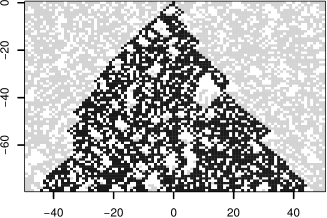
Figure 2.2. Left: A simulation of the space-time configuration of the stationary contact process $\eta$ from (2.3) with $p=0.68$. Dark sites have $\eta_{n}(x)=1$. Right: The same configuration with only those sites highlighted in dark which are potential ancestors of the individual at the origin $(\mathbf{0},0)$, i.e. those sites which the walk $X$ with dynamics (2.5) can reach.

The main result from [6] is the following theorem on the position $X_{n}$ of the random walk on the backbone of the oriented percolation cluster at time $n$. The theorem can be interpreted by saying that $X_{n}$ behaves similarly as a simple random walk: it satisfies a law of large numbers and a central limit theorem. (The case of simple random walk corresponds in our notation to $p=1$.) In other words, the percolation cluster behaves, on large scales, similarly as the full lattice: the effect of the ‘holes’ in the cluster – which are clearly visible in the simulation in Figure 2.2 – vanishes on large scales.

Theorem 2.1 (Law of large numbers, averaged and quenched central limit theorem, [6, Theorems 1.1. and 1.3]).

For any $d\geqslant 1$ we have

(2.6) $$P_{\omega}\Big{(}\frac{1}{n}X_{n}\to\mathbf{0}\,\Big{)}=1\quad\text{for $\mathbb{P}\hskip 0.5pt(\,\cdot\,|B_{0})$-a.a.\ $\omega$},$$

and for any $f\in C_{b}(\mathbb{R}^{d})$

(2.7) $$\mathbb{E}\Big{[}f\left(X_{n}/\sqrt{n}\,\right)\,\Big{|}\,B_{0}\Big{]}\xrightarrow{n\to\infty}\Phi(f),$$

(2.8) $$E_{\omega}\Big{[}f\left(X_{n}/\sqrt{n}\,\right)\,\Big{]}\xrightarrow{n\to\infty}\Phi(f)\quad\text{ for $\mathbb{P}\hskip 0.5pt(\,\cdot\,|B_{0})$-a.a.~{}$\omega$,}$$

where $\Phi(f):=\int f(x)\,\Phi(dx)$ with $\Phi$ a non-trivial centred isotropic $d$-dimensional normal law. Functional versions of (2.7) and (2.8) hold as well.

A proof sketch is given in Section 2.3 below.

Remark 2.2.

The covariance matrix of $\Phi$ in (2.7) is $\sigma^{2}$ times the $d$-dimensional identity matrix. It follows from the regeneration construction (see Subsection 2.3 below) that

(2.9) $$\sigma^{2}=\sigma^{2}(p)=\frac{\mathbb{E}\big{[}Y_{1,1}^{2}\big{]}}{\mathbb{E}[\tau_{1}]}\in(0,\infty)$$

where $\tau_{1}$ is the first regeneration time (see (2.15) below) of the random walk $X$ and $Y_{1,1}$ is the first coordinate of $X_{\tau_{1}}$, the position of the random walk at this regeneration time. The behaviour of $\sigma^{2}(p)$ as $p\downarrow p_{c}$ is an interesting open problem that merits further research.

Remark 2.3 (Consequences for the long-time behaviour of the multi-type process).

Let us enrich the contact process $(\eta_{n})_{n}$ from Section 2.1 by including (so-called neutral) types: Say, at time $n=0$, every $\eta_{0}(x)$ is independently assigned a uniformly chosen value from $(0,1)$ and we augment the rule (2.2) by setting $\eta_{n}(x)=\eta_{n-1}(y)>0$ if $y\in\mathcal{A}_{x,n}$ was chosen as the ancestor of the individual at site $(x,n)$. Thus, children inherit their parent’s type (which is $>0$) and we still interpret $\eta_{n}(x)=0$ as a vacant site. As $n\to\infty$, $\eta_{n}$ will converge in distribution to an equilibrium $\widetilde{\eta}$ of the multi-type dynamics.

It follows from Theorem 2.1 and its proof in [6] that any two ancestral lineages will eventually meet in $d\leqslant 2$, but not in $d\geqslant 3$. By ‘looking backwards in time’, this has consequences for $\widetilde{\eta}$: For any $x,y\in\mathbb{Z}\hskip 0.5pt$,

(2.10) $$\mathbb{P}\hskip 0.5pt\left(\widetilde{\eta}(x)=\widetilde{\eta}(y)\mid\widetilde{\eta}(x)>0,\widetilde{\eta}(y)>0\right)=1$$

in $d=1,2$ and this probability is $<1$ in $d\geqslant 3$. In fact, for $d\geqslant 3$ there is $C_{d}\in(0,\infty)$ such that

$$\mathbb{P}\hskip 0.5pt\left(\widetilde{\eta}(x)=\widetilde{\eta}(y)\mid\widetilde{\eta}(x)>0,\widetilde{\eta}(y)>0\right)\sim\frac{C_{d}}{\lVert x-y\rVert^{d-2}_{2}}\quad\text{as }\lVert x-y\rVert\to\infty.$$

These properties are analogous to those of the multi-type stepping stone model.

2.3. Proof ideas: Local construction and regeneration

A main difficulty in the proof of Theorem 2.1 lies in the fact that in order to determine $\xi(x,n)$, one has to know the ‘whole future’ of the environment $\omega$. To overcome this, we build a trajectory of $X$ using rules that are ‘local’, i.e. which use only local $\omega$’s (and some additional local randomness), but not the $\xi$’s. We then read off regeneration times from this construction: These are exactly the times when the locally constructed trajectory coincides with the true trajectory of $X$, see (2.14) below. This approach is inspired by [29] and [34].

The construction employs some additional randomness: For every $(x,n)\in\mathbb{Z}\hskip 0.5pt^{d}\times\mathbb{Z}\hskip 0.5pt$ let $\widetilde{\omega}{(x,n)}$ be a uniformly chosen permutation of $U(x,n)$ ($U(x,n)$ may be written as a vector by ordering the elements according to the lexicographical ordering of the space ccordinate $x$), independently distributed for all $(x,n)$’s and independent from the $\omega$’s. We denote the whole family of these permutations by $\widetilde{\omega}$.

For every $(x,n)\in\mathbb{Z}^{d}\times\mathbb{Z}$ let $\ell(x,n)=\ell_{\infty}(x,n)$ be the length of the longest directed open path starting at $(x,n)$; we set $\ell(x,n)=-1$ when $(x,n)$ is closed. (Recall that a path $(x_{0},n),(x_{1},n+1),\dots,(x_{k},n+k)$ of length $k$ with $\lVert{x_{i}-x_{i-1}}\rVert\leqslant 1$ is open if $\omega(x_{0},n)=\omega(x_{1},n+1)=\cdots=\omega(x_{k},n+k)=1$. $\ell(x,n)=\infty$ means $(x,n)\in\mathcal{C}$.) For every $k\in\mathbb{N}_{0}$ let $\ell_{k}(x,n):=\ell(x,n)\wedge k$ be the length of the longest directed open path of length at most $k$ starting from $(x,n)$. Observe that $\ell_{k}(x,n)$ is measurable with respect to the $\sigma$-algebra $\mathcal{G}_{n}^{n+k+1}$, where

(2.11) $$\mathcal{G}_{n}^{m}:=\sigma\big{(}\omega(y,i),\widetilde{\omega}{(y,i)}:y\in\mathbb{Z}\hskip 0.5pt^{d},n\leqslant i<m\big{)},\quad n<m.$$

For $k\in\{0,\dots,\infty\}$, we define $M_{k}(x,n)\subseteq U(x,n)$ to be the set of sites which maximise $\ell_{k}$ over $U(x,n)$, i.e.

$$M_{k}(x,n):=\Big{\{}y\in U(x,n):\ell_{k}(y)=\max_{z\in U(x,n)}\ell_{k}(z)\Big{\}},$$

and for convenience we set $M_{-1}(x,n)=U(x,n)$. Observe that we have

$$M_{0}(x,n) =\{y\in U(x,n):y\text{ is open}\},$$

$$M_{\infty}(x,n) =U(x,n)\cap\mathcal{C},$$

$$M_{k}(x,n) \supseteq M_{k+1}(x,n),\qquad k\geqslant-1.$$

Let $m_{k}(x,n)\in M_{k}(x,n)$ be the element of $M_{k}(x,n)$ that appears as the first in the permutation $\widetilde{\omega}{(x,n)}$.

Given $(x,n)$, $k$, $\omega$ and $\widetilde{\omega}$, we define a path $\gamma_{k}=\gamma_{k}^{(x,n)}$ of length $k$ via

(2.12) $$\gamma_{k}(0)=(x,n),\qquad\gamma_{k}(j+1)=m_{k-j-2}(\gamma_{k}(j))\;\;\text{for }j=0,\dots,k-1.$$

In words, at every step, $\gamma_{k}$ checks the neighbours of its present position and picks randomly (using the random permutation $\widetilde{\omega}$) one of those where it can go further on open sites, but inspecting only the state of sites in the time-layers $\{n,\dots,n+k-1\}$. Consequently, the construction of $\gamma_{k}^{(x,n)}$ is measurable with respect to the $\sigma$-algebra $\mathcal{G}_{n}^{n+k}$ from (2.11). See Figure 2.3 for an illustration. Intuitively, $\gamma_{k}^{(x,n)}$ would be the trajectory of $X$ starting from the space-time point $(x,n)$ if we replaced in (2.5) the condition that $X$ can only walk on $\mathcal{C}$ by the requirement that the first $k$ steps must begin on open sites.

Figure 2.3. The paths $\gamma_{k}^{(x,n)}$ from (2.12) based on $\omega$’s and $\widetilde{\omega}$’s. Black and white circles represent open sites, i.e. $\omega(\text{site})=1$, and closed sites, i.e. $\omega(\text{site})=0$, respectively. Solid arrows from a site point to $\widetilde{\omega}_{(\text{site})}(1)$ and dotted to $\widetilde{\omega}_{(\text{site})}(2)$. On the right the sequence of paths $\gamma_{k}^{(x,n)}(\cdot)$ for $k=1,2,3,4$ is shown. For sake of pictorial clarity, we used here $U(x,n)=\{(x+1,n+1),(x-1,n+1)\}$ here instead of (2.4).

It is not hard to check that these paths $\gamma_{k}^{(x,n)}$ have the following properties (see [6, Lemma 2.1 and Remark 2.2] for details): Given $\omega$, $(x,n)\in\mathcal{C}$ and $\widetilde{\omega}$,

• (steps begin on open sites) $\omega(\gamma_{k}(m))=1$ for all $0\leqslant m<k$.

• (stability in $k$) If the end point of $\gamma_{k}$ is open, i.e. $\omega(\gamma_{k}(k))=1$, then the path $\gamma_{k+1}$ restricted to the first $k$ steps equals $\gamma_{k}$.

• (fixation on $\mathcal{C}$) Assume that $\gamma_{k}(j)\in\mathcal{C}$ for some $k\geqslant 0$, $j\leqslant k$. Then, $\gamma_{m}(j)=\gamma_{k}(j)$ for all $m>k$.

• (exploration of finite branches) If $\gamma_{k}(k-1)\in\mathcal{C}$ and $\gamma_{k}(k)\notin\mathcal{C}$ for some $k$, then $\gamma_{j}(k)=\gamma_{k}(k)$ for all $k\leqslant j\leqslant k+\ell(\gamma_{k}(k))+1$ and $\gamma_{k+\ell(\gamma_{k}(k))+2}(k)\neq\gamma_{k}(k)$.

By (c), $\gamma_{\infty}^{(x,n)}(j)=\lim_{k\to\infty}\gamma_{k}(j)$ exists a.s. (since holes in the cluster are a.s. finite). Furthermore, for fixed $\omega$ and $(x,n)\in\mathcal{C}$ (but thinking of $\widetilde{\omega}$ as random), the law of $(\gamma_{\infty}^{(x,n)}(j))_{j\geqslant 0}$ is the same as the law of the random walk $(X_{j},n+j)_{j\geqslant 0}$ on $\mathcal{C}$ started from $(x,n)$. Thus we can and shall couple the random walk $(X_{k},k)$ started from $(\boldsymbol{0},0)$ with the random variables $\omega,\widetilde{\omega}$ by setting

(2.13) $$(X_{k},k)=\gamma_{\infty}^{(\boldsymbol{0},0)}(k)=\lim_{j\to\infty}\gamma_{j}^{(\boldsymbol{0},0)}(k).$$

With these ingredients, we can define regeneration times as follows: Let

(2.14) $$T_{0}:=0\quad\text{and}\quad T_{j}:=\inf\left\{k>T_{j-1}:\xi(\gamma^{(\boldsymbol{0},0)}_{k}(k))=1\right\},\quad j\geqslant 1.$$

(Here and later we use the notation $\xi(y):=\xi_{n}(x)$ when $y=(x,n)\in\mathbb{Z}^{d}\times\mathbb{Z}$.) At times $T_{j}$ the local construction of the path finds a ‘real ancestor’ of $(\boldsymbol{0},0)$ in the sense that for any $m>T_{j}$, $\gamma^{(\boldsymbol{0},0)}_{m}(T_{j})=\gamma^{(\boldsymbol{0},0)}_{T_{j}}(T_{j})$, by property (c). The increments between regeneration times are

(2.15) $$\tau_{i}:=T_{i}-T_{i-1}\qquad\text{and}\qquad Y_{i}:=X_{T_{i}}-X_{T_{i-1}}.$$

and we then indeed have that

(2.16) $$\text{the sequence $\bigl{(}(Y_{i},\tau_{i})\bigr{)}_{i\geqslant 1}$ is i.i.d.\ and $Y_{1}$ is symmetrically distributed},$$

(2.17) $$\text{both $Y_{1}$ and $\tau_{1}$ have exponential tails}.$$

The intuition behind the regeneration property (2.16) is the following: Assume that for some $k$, we have constructed the path $\gamma_{k}^{(\boldsymbol{0},0)}$ and observe that $\xi\big{(}\gamma_{k}^{(\boldsymbol{0},0)}(k)\big{)}=1$. Then we have obtained information about some $\omega(y,j)$ and $\widetilde{\omega}(y,j)$ for $j<k$, $y\in\mathbb{Z}\hskip 0.5pt^{d}$ and we know that the site $\gamma_{k}^{(\boldsymbol{0},0)}(k)$ in time-slice $k$ is connected to $+\infty$. The latter property depends only on $\omega(y,j)$ with $j\geqslant k$, $y\in\mathbb{Z}\hskip 0.5pt^{d}$ and the $\omega$’s in different time-slices are independent. By property (c), we have $(X_{k},k)=\gamma_{k}^{(\boldsymbol{0},0)}(k)$. Thus, concerning the future behaviour of $X$, we are then at time $k$ in the same situation as at time $0$: All we know (and need to know) is that $X$ sits on some site in $\mathcal{C}$, and we can start afresh.

However, if we observe that $\xi\big{(}\gamma_{k}^{(\boldsymbol{0},0)}(k)\big{)}=0$, we are in a different situation: We then know that $\gamma_{k}^{(\boldsymbol{0},0)}(k)$ is the starting point of a finite (possibly empty) oriented percolation cluster. Then we must continue the local construction until it has explored the ‘reason why $\xi\big{(}\gamma_{k}^{(\boldsymbol{0},0)}(k)\big{)}=0$’, which depends on finitely many sites (cf property (d) above).

See Figure 2.4 for an illustration: In this example, the local construction enters a finite cluster at time $k=\sigma_{1}$ and explores this, regeneration occurs then at time $T_{1}=\sigma_{2}$ when the exploration is completed. The full details are in [6, Lemma 2.5].

To obtain (2.17), one uses the fact that the height of a finite cluster in supercritical oriented percolation has exponential tails, see [17] and [6, Lemma A.1]. The distributional symmetry of $Y_{1}$ follows from the symmetry of $U(x,n)$ in (2.4).

Figure 2.4. ‘Discovering’ of the trajectory of $X$ between the regeneration times $T_{0}$ and $T_{6}$ in case $U=\{-1,1\}$ is shown on the left-hand side of the figure. On the right-hand side we zoom into the evolution between $T_{0}$ and $T_{1}$. On the two ‘relevant sites’ we show the realisation of $\widetilde{\omega}$’s using the same conventions as in Figure 2.3 (in particular, again $U(x,n)=\{(x+1,n+1),(x-1,n+1)\}$).

Given (2.16) and (2.17), the law of large numbers (2.6) and the annealed CLT (2.7) follow straightforwardly by re-writing $X_{n}$ as a sum along regeneration times plus an asymptotically negligible remainder. The quenched CLT (2.8) requires some additional effort: Here, we used two copies $X$ and $X^{\prime}$ of the walk on the same cluster $\mathcal{C}$ to control the variance of $E_{\omega}\big{[}f\left(X_{n}/\sqrt{n}\,\right)\,\big{]}$, an approach inspired by [16]. This, in turn, requires to enlarge the regeneration construction to incorporate simultaneous regenerations for both $X$ and $X^{\prime}$. Studying two (or more) copies of the walk on $\mathcal{C}$, especially when one stipulates that they coalesce as soon as they meet, is also very natural from the point of view of larger samples. In fact, this is exactly the device that is made use of in [8] and it also plays a key role in the proof of (2.20) below. We will however not spell out the details here and instead refer to [6, 8].

2.4. Extensions

2.4.1. Contact process with fluctuating population sizes

Let $K(x,n)$, $(x,n)\in\mathbb{Z}\hskip 0.5pt^{d}\times\mathbb{Z}\hskip 0.5pt$ be possibly correlated $\mathbb{N}$-valued random variables, independent of the $\omega$’s. We define the discrete time contact process with fluctuating population size, $\widehat{\eta}:=(\widehat{\eta}_{n})_{n\in\mathbb{Z}\hskip 0.5pt}$, by

(2.18) $$\widehat{\eta}_{n}(x):=\eta_{n}(x)K(x,n),$$

with $\eta_{n}(x)$ from (2.3) and its time reversal $\widehat{\xi}:=(\widehat{\xi}_{n})_{n\in\mathbb{Z}\hskip 0.5pt}$ by $\widehat{\xi}_{n}(x):=\xi_{n}(x)K(x,n).$

One can interpret $K(x,n)$ as a random ‘carrying capacity’ of the site $(x,n)$: When $\eta_{n}(x)=1$, $K(x,n)$ individuals live at position $x$ in generation $n$, and each of them is independently assigned an ancestor from $\mathcal{A}_{x,n}$ as in (2.2).

Now conditioned on $\widehat{\xi}_{0}(\mathbf{0})\geqslant 1$ the ancestral random walk is defined by $X_{0}=\boldsymbol{0}$ and (2.5) is generalised to

(2.19) $$\mathbb{P}\hskip 0.5pt\bigl{(}X_{n+1}=y\mid X_{n}=x,\widehat{\xi}\,\bigr{)}=\begin{cases}\dfrac{\widehat{\xi}_{n+1}(y)}{\sum_{(y^{\prime},n+1)\in U(x,n)}\widehat{\xi}_{n+1}(y^{\prime})}\;\;&\text{if }(y,n+1)\in U(x,n),\\[11.38109pt] 0&\text{otherwise.}\end{cases}$$

Analogues of Theorem 2.1 then hold under suitable assumptions on the random field $K=(K(x,n))_{x\in\mathbb{Z}\hskip 0.5pt^{d},n\in\mathbb{Z}\hskip 0.5pt}.$ The case when $K$ is an i.i.d. field is discussed in [6, Remark 1.6]. K. Miller [32] generalises this considerably by assuming instead certain mixing conditions: A law of large numbers analogous to (2.6), with possibly non-zero speed, holds if $K$ is $\phi$-mixing in time with coefficients $\phi_{n}\in O(n^{-1-\delta})$ for some $\delta>0$, an annealed CLT analogous to (2.7) holds if $\phi_{n}\in O(n^{-2-\delta})$; a quenched CLT analogous to (2.7) holds if $K$ is exponentially mixing in space and time. Note that in general, (2.19) describes a non-elliptic random walk in a non-Markovian (but mixing) environment. The key idea is again a ‘regeneration construction’ where the i.i.d. property in (2.16) is now replaced by a sufficiently strong mixing property. We refer to [32] and [33] for details.

2.4.2. Brownian web limit in spatial dimension one

One can consider the ancestral lineages of all individuals in the stationary $\eta$ from (2.3) simultaneously. This gives rise to an infinite system of random walks $X^{(x,n)}=(X^{(x,n)}_{m})_{m\geqslant n}$ on the time-reversal $\xi$ of $\eta$, where for each $(x,n)\in\mathcal{C}$, the walk $X^{(x,n)}$ starts at time $n$ at position $x$, follows the analogue of (2.5), and different walkers coalesce whenever they meet in the same space-time site. By Theorem 2.1 and space-time stationarity, any $X^{(x,n)}$ converges to a Brownian motion under diffusive rescaling. As shown in [8], in spatial dimension $d=1$, the collection of all these paths converges after diffusive rescaling as in Theorem 2.1 in distribution to the Brownian web. Informally, this limit object describes an infinite system of coalescing Brownian motions starting from all space-time points in $\mathbb{R}\times\mathbb{R}$. One may then apply our convergence result to investigate the behaviour of interfaces in the discrete time contact process analogously to [36, Theorem 7.6 and Remark 7.7], as observed in [8, p. 1051]. We refer also to the article ‘Interfaces in spatial population dynamics’ by Marcel Ortgiese in this volume, which studies spatial population models (in continuous space) in $d=1$, with a particular focus on interfaces. These models are ‘continuum analogues’ of the voter model, and the interfaces are stochastic processes in dynamic environments. Dualities and their genealogical interpretations play an important role there as well.

An important ingredient in the proof is a quantitative strengthening of (2.10) from Remark 2.3:

(2.20) $$\mathbb{P}\hskip 0.5pt\left(T^{(z_{1},z_{2})}_{\mathrm{meet}}>n\,\Big{|}\,\xi_{0}(z_{1})=\xi_{0}(z_{2})=1\right)\leqslant\text{const.}\times\frac{|z_{1}-z_{2}|}{\sqrt{n}}\quad\text{for }z_{1},z_{2}\in\mathbb{Z}\hskip 0.5pt,\,n\in\mathbb{N},$$

where $T^{(z_{1},z_{2})}_{\mathrm{meet}}$ is the number of steps until two walks on the same realisation of $\xi$ which start at time $0$ from $z_{1}$ and $z_{2}$, respectively, meet for the first time. Note that (2.20) is the asymptotically correct form of the decay for simple random walks in $d=1$. For more information, we refer to [40].

The results in [8] can again be interpreted as an averaging statement about the percolation cluster: apart from a change of variance, it behaves as the full lattice (for which convergence to the Brownian web was proved in [36]), i.e. the effect of the ‘holes’ in the cluster vanishes on a large scale. For a thorough discussion of the Brownian web, including historical comments and references, see the overview article [39]. Note that there is no analogous object in spatial dimension $d\geqslant 2$ because there, independent Brownian motions never meet.

3. Ancestral lineages for logistic branching random walks

We consider a system of discrete-time branching random walks with logistic regulation: Let $\eta_{n}(x)$ be the number of individuals at position $x\in\mathbb{Z}\hskip 0.5pt^{d}$ in generation $n\in\mathbb{Z}\hskip 0.5pt$. Given the configuration $\eta_{n}$ at time $n$, for $x\in\mathbb{Z}\hskip 0.5pt^{d}$, each individual at $x$ has a Poisson-distributed number of offspring with mean

(3.1) $$\big{(}m-\sum_{z}\lambda_{z-x}\eta_{n}(z)\big{)}^{+}$$

and each child moves to $y$ with probability $p_{y-x}$, independently for different parental individuals and for different children. Here, $p_{xy}=p_{y-x}$ is a symmetric, aperiodic finite range random walk kernel on $\mathbb{Z}\hskip 0.5pt^{d}$, $m>1$, $\lambda_{z}\geqslant 0$, $z\in\mathbb{Z}\hskip 0.5pt^{d}$ is symmetric with finite range and $\lambda_{0}>0$. These children then form the next generation, $\eta_{n+1}$. (3.1) has a natural interpretation as local competition: each individual at $z$ reduces the average reproductive success of a focal individual at $x$ by $\lambda_{z-x}$. In particular, this introduces local density-dependent feedback in the model: The offspring distribution is supercritical when there are few neighbours and subcritical when there are many neighbours. Note that by properties of the Poisson distribution $(\eta_{n})$ is in fact a probabilistic cellular automaton: Given $\eta_{n}$,

(3.2) $$\eta_{n+1}(y)\sim\mathrm{Poisson}\left({\sum\limits_{x\in\mathbb{Z}\hskip 0.5pt^{d}}}\big{(}m-\sum_{z\in\mathbb{Z}\hskip 0.5pt^{d}}\lambda_{z-x}\eta_{n}(z)\big{)}^{+}p_{y-x}\right),$$

independently for different $y\in\mathbb{Z}\hskip 0.5pt^{d}$.

Remark 3.1.

1. For the choice $\lambda\equiv 0$, the system $(\eta_{n})_{n}$ is a ‘classical’ branching random walk, in which different individuals behave completely independently. This is a classical topic with a lot of recent progress, see in particular the article ‘Branching random walks in random environment’ by Wolfgang König in this volume. In [23] and [24], moment asymptotics for the number of particles in a branching random walk in random environment are derived. Note that the first moments correspond to the well-investigated solutions of the parabolic Anderson model.

2. Conditioning on $\eta_{n}(\cdot)\equiv N$ in (3.2) for some $N\in\mathbb{N}$ and considering types and/or ancestral relationships, as we will do below, yields a version of the stepping stone model.

3. The form of the competition kernel and the Poisson offspring law in (3.1)–(3.2) are prototypical (and convenient for the proofs) but can be replaced by more general choices, see the discussion in [5, Remark 5 (ii)] and [7, Section 5].

Theorem 3.2 (Survival and complete convergence, [5, Theorem 1 and Corollary 4]).

Assume $m\in(1,3)$. There exist $\varepsilon_{0},\varepsilon_{1}>0$ such that for all choices $0<\lambda_{0}\leqslant\varepsilon_{0}$ and $0\leqslant\lambda_{z}\leqslant\varepsilon_{1}\lambda_{0}$ for $z\neq 0$, the system $(\eta_{n})$ survives for all time locally (and hence also globally) with positive probability for any non-trivial initial condition $\eta_{0}$. Given survival (either local or global), $\eta_{n}$ converges as $n\to\infty$ in distribution to its unique non-trivial equilibrium.

We will not prove Theorem 3.2 here but point out that a crucial ingredient in the proof is a strong coupling property of the system $(\eta_{n})$: Starting from any two initial conditions $\eta_{0}$, $\eta_{0}^{\prime}$,

(3.3) copies $$(\eta_{n}) (\eta^{\prime}_{n}) \eta_{n}(x)=\eta^{\prime}_{n}(x)$$, can be coupled such that if both survive, in a space-time cone.

This allows to compare the system to supercritical oriented percolation on suitably coarse-grained space-time scales, see [5, Section 5] for details and see Figure 3.1 for a simulation.

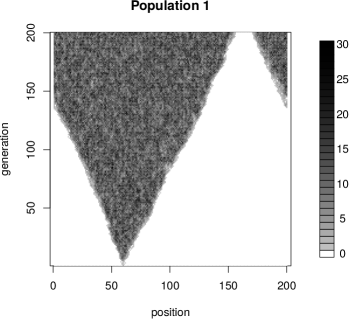
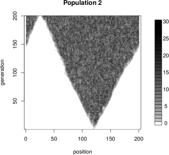
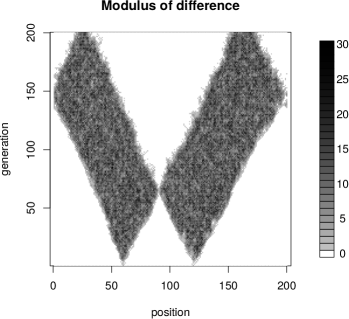
Figure 3.1. Starting from any two initial conditions $\eta_{0}$, $\eta_{0}^{\prime}$, copies $(\eta_{n})$, $(\eta^{\prime}_{n})$ can be coupled such that if both survive (here, $m=1.5$, $p=(1/3,1/3,1/3)$, $\lambda=(0.01,0.02,0.01)$, $\eta_{0}=\delta_{60}$, $\eta_{0}^{\prime}=\delta_{120}$ and space is $\{1,2,\dots,200\}$ with periodic boundary conditions). The picture at the bottom shows $|\eta_{n}(x)-\eta_{n}^{\prime}(x)|$, note the growing region in the middle where $\eta_{n}(x)=\eta_{n}^{\prime}(x)>0$.

Remark 3.3.

1. The restriction to $m<3$ in Theorem 3.2 is ‘inherited’ from the logistic iteration $w_{n+1}=mw_{n}(1-w_{n})$ because in this parameter regime, it has a unique attracting fixed point. Note that literally, a ‘deterministic space-less’ analogue of (3.2) would read $\widetilde{w}_{n+1}=m\widetilde{w}_{n}(1-\tilde{\lambda}\widetilde{w}_{n})$ with $\tilde{\lambda}=\sum_{z}\lambda_{z}$, the rescaling $\widetilde{w}_{n}=(m/\tilde{\lambda})w_{n}$ brings this to the ‘standard form’ just mentioned.

Survival can be proved also for $m\in[3,4)$ with similar arguments, but convergence cannot. For $m<1$ (and for $m=1$ in $d\leqslant 2$) one can easily see, using domination by subcritical branching random walks, that $(\eta_{n})_{n}$ will die out locally when starting from any initial condition $\eta_{0}$ with $\sup_{x\in\mathbb{Z}\hskip 0.5pt^{d}}\mathbb{E}[\eta_{0}(x)]<\infty$.

2. In [21], multi-type continuous mass branching populations with competitive interactions are studied, the logistic branching random walks we described in Section 3 are a close relative of such systems in the single-type case (or in the multi-type case with completely symmetric parameters). Furthermore, by using space $\mathbb{R}^{d}$ as a ‘trait space,’ the measure-valued processes studied in [4] can be seen as a suitable scaling limit of (relatives of) logistic branching random walks, see [4, Remark 5]. Many challenging questions about the long-time behaviour of such continuous-mass interacting multi-type systems remain open. It is conceivable that the regeneration constructions for ancestral lineages we investigated in [6] and [7] might be adaptable to this context, and that this could enrich the pertinent ‘tool box.’

3.1. Dynamics of an ancestral lineage

By Theorem 3.2, for suitable choices of the parameters, the system (3.2) has a unique non-trivial equilibrium. We denote by $\eta^{\rm stat}=(\eta^{\rm stat}_{n}(x))_{n\in\mathbb{Z}\hskip 0.5pt,x\in\mathbb{Z}\hskip 0.5pt^{d}}$ the corresponding stationary process and – implicitly in our notation – ‘enrich’ it suitably to allow bookkeeping of genealogical relationships, as described at the beginning of Section 3. Consider the stationary $\eta^{\rm stat}$ conditional on $\eta^{\rm stat}_{0}(\mathbf{0})>0$ and sample an individual (uniformly) from the space-time origin $(\mathbf{0},0)$, let $X_{n}$ be the spatial position of her ancestor $n$ generations ago. Then

(3.4) $$\mathbb{P}\hskip 0.5pt\big{(} X_{n+1}=y\,\big{|}\,X_{n}=x,\eta^{\rm stat}\big{)}=\frac{p_{x-y}\eta^{\rm stat}_{-n-1}(y)\big{(}m-{\textstyle\sum_{z}\lambda_{z-y}\eta^{\rm stat}_{-n-1}(z)}\big{)}^{+}}{\sum_{y^{\prime}}p_{x-y^{\prime}}\eta^{\rm stat}_{-n-1}(y^{\prime})\big{(}m-{\textstyle\sum_{z}\lambda_{z-y^{\prime}}\eta^{\rm stat}_{-n-1}(z)}\big{)}^{+}},$$

see [7, (4.10–4.11)].

Thus $(X_{n})_{n}$ is a random walk in a – relatively complicated – random environment. Note that the forwards in time direction for the walk corresponds to backwards in time for $\eta^{\rm stat}$. Again it turns out that $X$ behaves like ordinary random walk when viewed over large enough space-time scales, as the following theorem shows.

Theorem 3.4 (Law of large numbers and (averaged) central limit theorem, [7, Theorem 4.3]).

Assume $m\in(1,3)$. There exist $\varepsilon_{0},\varepsilon_{1}>0$ such that for all choices $0<\lambda_{0}\leqslant\varepsilon_{0}$ and $0\leqslant\lambda_{z}\leqslant\varepsilon_{1}\lambda_{0}$ for $z\neq 0$, we have

(3.5) $$\mathbb{P}\hskip 0.5pt\Big{(}\frac{1}{n}X_{n}\to\mathbf{0}\,\Big{|}\,\eta_{0}^{\rm stat}(\mathbf{0})\neq 0\Big{)}=1$$

and

(3.6) $$\mathbb{E}\Big{[}f\big{(}\tfrac{1}{\sqrt{n}}X_{n}\big{)}\,\Big{|}\,\eta_{0}^{\rm stat}(\mathbf{0})\neq 0\Big{]}\mathop{\longrightarrow}_{n\to\infty}\mathbb{E}\big{[}f(Z)\big{]}$$

for $f\in C_{b}(\mathbb{R}^{d})$, where $Z$ is a (non-degenerate) $d$-dimensional normal random variable. A functional version of (3.6) holds as well.

Note that (3.6) is an averaged limit result. In ongoing work with Andrej Depperschmidt and Timo Schlüter, we are proving the corresponding ‘quenched’ limit theorem.

The proof of Theorem 3.4 employs again a regeneration construction and a decomposition as in (2.15). We will only sketch the main ideas below, referring the reader to [7] for details.

Given $\eta^{\rm stat}$, $X$ is a time-inhomogeneous Markov chain; given also $X_{n}=x$ its transition probabilities in the $n+1$-th step depend only on $\eta^{\rm stat}_{-n-1}(x)$ in some finite window around $x$. We see from (3.4) that these transition probabilities are close to the fixed reference law $(p_{x})_{x}$ if $X_{n}$ is in a region where the relative variation of $\eta_{-n-1}(X_{n})$ is small.

Thus, we define ‘good’ space-time blocks in $\eta^{\rm stat}$ on suitable length scales $L_{\rm space}\gg 1$ and $L_{\rm time}\gg 1$, that is a finite set $\mathcal{G}$ of local configurations on $\{1,2,\dots,L_{\rm space}\}^{d}\times\{1,2,\dots,L_{\rm time}\}$ with the properties that

• $\eta^{\rm stat}$ has small relative variations inside a good block,

• if the block with (coarse grained) index $(\tilde{x},\tilde{n})\in\mathbb{Z}\hskip 0.5pt^{d}\times\mathbb{Z}\hskip 0.5pt$ is good, this will with high probability also be the case for its ‘temporal successors’ with indices $(\tilde{x}-1,\tilde{n}+1),(\tilde{x},\tilde{n}+1),(\tilde{x}+1,\tilde{n})$,

• if we consider two copies $\eta$ and $\eta^{\prime}$ of the system (3.2) with the property that in both the block with (coarse grained) index $(\tilde{x},\tilde{n})$ is good, then with high probability the coupling discussed in (3.3) will make $\eta$ and $\eta^{\prime}$ identical on the block with index $(\tilde{x},\tilde{n}+1)$.

(a) allows to control the walk $X$ whenever it moves through good blocks; (b) allows to compare the good blocks to supercritical oriented percolation (on the coarse-grained scale); (c) allows to ‘localise’ information about the space-time configuration $\eta^{\rm stat}$ around good blocks, this is akin to the local construction from Section 2.3.

With these ingredients, we can discuss the regeneration construction: Assume that we find a space-time ‘cone’ $C$ (with fixed suitable base diameter and slope) which is centred at the current space-time position $(X_{n},-n)$ of the walk such that

• $C$ covers the path and everything it has ‘explored’ until the $n$-th step (since the last regeneration),

• the configuration in $\eta^{\rm stat}$ at the base of the cone $C$ is ‘good’ and

• ‘strong’ coupling for $\eta^{\rm stat}$ as defined in property (c) above occurs inside the cone $C$.

Then, the conditional law of the future path increments is completely determined by the configuration $\eta^{\rm stat}$ at the base of the cone and we can ‘start afresh.’ It may happen that in order to find a cone with properties (i)–(iii), several attempts are needed, see Figure 3.2 for an illustration.

This construction expresses the path increments between the regeneration times as a functional of a well-behaved Markov chain (which keeps track of the local configuration at the base of the corresponding cones at the regeneration times). Given this, (3.5) and (3.6) are fairly standard.

Figure 3.2. A schematic illustration of the regeneration construction for Theorem 3.4: The walk passes through a sequence of cones in an attempt to regenerate. Here, regeneration at time $t_{1}$ fails because the path up to that time is not covered by the corresponding cone and regeneration at time $t_{2}$ fails because the corresponding cone does not cover the previous cone; successful regeneration then occurs in the third attempt at time $t_{3}$.

In ongoing work with Andrej Depperschmidt and Timo Schlüter we consider the joint dynamics of several ancestral lineages in the logistic branching random walk and establish properties analogous to those in Section 2.2 for walks on the oriented percolation cluster.

4. Discussion

Our ancestral walks with dynamics as in (2.5), (2.19), (3.4) are generally speaking random walks in dynamical random environments (RWDRE). This is currently a very active field of research and we do not attempt to give an overview here, but refer to [1] for a good overview of the area up to 2010. There are recent papers on random walks in dynamical random conductances, random walks on dynamical percolation, random walks in dynamical random environments given by interacting particle systems as for instance exclusion processes. The general results have often strong assumptions on the environment (mixing conditions, spectral gap assumptions, uniform lower bounds for the transition probabilities of the walk). On the other hand, the ‘case studies’ often refer to specific models and do not provide a general approach. Hence, this is an area where there is still a lot to understand. See, e.g., the recent works [2, 13] and the discussion and references there. Let us point out that our walks (2.5), (2.19), (3.4) are somewhat special inside the general class of RWDRE in that the natural ‘forwards’ time direction for the walk is ‘backwards’ in time for the environment, whereas often researchers in RWDRE study walks on certain interacting particle systems where the walk and the underlying system have the same forwards time direction. Also, let us mention that while in recent work, see [10], the assumption of ellipticity of the environment, i.e. on uniform lower bounds for the transition probabilities of the walk, is not present anymore, our model still does not fit in, since our environment is not stationary.

Acknowledgements. The authors thank Jiří Černý, Andrej Depperschmidt, Katja Miller and Sebastian Steiber for the many enlightening discussions we had in the course of this project. We would also like to thank Iulia Dahmer, Frederik Klement and Timo Schlüter and an anonymous referee for carefully reading the manuscript and for their helpful comments.

References

- [1] L. Avena, Random walks in dynamic random environments, Proefschrift Universiteit Leiden (PhD dissertation), 2010. http://hdl.handle.net/1887/16072
- [2] L. Avena, O. Blondel, A. Faggionato, Analysis of random walks in dynamic random environments via -perturbations, Stoch. Proc. Appl. 128 (2018), 3490–3530.
- [3] N. H. Barton, F. Depaulis, and A. M. Etheridge, Neutral evolution in spatially continuous populations. Theoret. Popul. Biol. 61 (2002), 31 – 48.
- [4] G. Berzunza, A. Sturm, A. Winter, Trait-dependent branching particle systems with competition and multiple offspring, preprint, arXiv:1808.09345.
- [5] M. Birkner and A. Depperschmidt, Survival and complete convergence for a spatial branching system with local regulation. Ann. Appl. Probab. 17 (2007), 1777–1807.
- [6] M. Birkner, J. Černý, A. Depperschmidt and N. Gantert, Directed random walk on the backbone of an oriented percolation cluster, Electron. J. Probab. 18 (2013), no. 80, 35p.
- [7] M. Birkner, J. Černý and A. Depperschmidt, Random walks in dynamic random environments and ancestry under local population regulation, Electron. J. Probab. 21 (2016), no. 38, 1–43.
- [8] M. Birkner, N. Gantert and S. Steiber, Coalescing directed random walks on the backbone of a 1+1-dimensional oriented percolation cluster converge to the Brownian web, ALEA Lat. Am. J. Probab. Math. Stat. 16 (2019), 1029–1054.
- [9] M. Birkner, R. Sun, Low-dimensional lonely branching random walks die out, Ann. Probab. 47 (2019), 774–803.
- [10] M. Biskup, P.-F. Rodriguez, Limit theory for random walks in degenerate time-dependent random environments, Journal of Functional Analysis 274 (2018), 985–1046.
- [11] J. Blath, A. M. Etheridge, and M. Meredith, Coexistence in locally regulated competing populations and survival of branching annihilating random walk, Ann. Appl. Probab. 17 (2007), 1474–1507.
- [12] J. Blath, M. Hammer, M. Ortgiese, The scaling limit of the interface of the continuous-space symbiotic branching model, Ann. Probab. 44 (2016), 807–866.
- [13] O. Blondel, M. R. Hilário, A. Teixeira, Random Walks on Dynamical Random Environments with Non-Uniform Mixing, preprint, arXiv:1805.09750.
- [14] B. M. Bolker, S. W. Pacala Using moment equations to understand stochastically driven spatial pattern formation in ecological systems, Theoret. Popul. Biol. 52, (1997) 179–197.
- [15] B. M. Bolker, S. W. Pacala, Spatial moment equations for plant competition: Understanding spatial strategies and the advantages of short dispersal, American Naturalist 153, (1999) 575–602.
- [16] E. Bolthausen and A.-S. Sznitman, On the static and dynamic points of view for certain random walks in random environment, Methods Appl. Anal. 9 (2002), 345–375, Special issue dedicated to Daniel W. Stroock and Srinivasa S. R. Varadhan on the occasion of their 60th birthday.
- [17] R. Durrett, Oriented percolation in two dimensions, Ann. Probab. 12 (1984), 999–1040.
- [18] A. M. Etheridge, Survival and extinction in a locally regulated population. Ann. Appl. Probab. 14 (2004), 188–214.
- [19] A. M. Etheridge, Some mathematical models from population genetics, Volume 2012 of Lecture Notes in Mathematics, Springer, 2011. Lectures from the 39th Probability Summer School held in Saint-Flour, 2009.
- [20] N. Fournier, S. Méléard, A microscopic probabilistic description of a locally regulated population and macroscopic approximations. Ann. Appl. Probab. 14 (2004), 1880–1919.
- [21] A. Greven, A. Sturm, A. Winter and I. Zähle, Multi-type spatial branching models for local self-regulation I: Construction and an exponential duality, preprint, arXiv:1509.04023.
- [22] G. Grimmett and P. Hiemer, Directed percolation and random walk, In and out of equilibrium (Mambucaba, 2000), Progr. Probab., vol. 51, Birkhäuser, 2002, pp. 273–297.
- [23] O. Gün, W. König, O. Sekulović, Moment asymptotics for branching random walks in random environment. Electron. J. Probab. 18 (2013), no. 63, 1–18.
- [24] O. Gün, W. König, O. Sekulović, Moment asymptotics for multitype branching random walks in random environment. J. Theoret. Probab. 28 (2015), 1726–1742.
- [25] M. Hammer, M. Ortgiese, F. Völlering, A new look at duality for the symbiotic branching model, Ann. Probab. 46 (2018), 2800–2862.
- [26] M. Hammer, M. Ortgiese, F. Völlering, Entrance laws for annihilating Brownian motions and the continuous-space voter model, preprint, arXiv:1801.06197.
- [27] M. Hutzenthaler, A. Wakolbinger, Ergodic behaviour of locally regulated branching populations. Ann. Appl. Probab. 17 (2007), 474–501.
- [28] O. Kallenberg, Stability of critical cluster fields. Math. Nachr. 77 (1977), 7–43.
- [29] T. Kuczek, The central limit theorem for the right edge of supercritical oriented percolation, Ann. Probab. 17 (1989), 1322–1332.
- [30] R. Law, U. Dieckmann Moment approximations of individual-based models. In U. Dieckmann, R. Law, and J. A. Metz (Eds.) The Geometry of Ecological Interactions, Cambridge Univ. Press, 2002, pp. 252–270.
- [31] V. Le, E. Pardoux, and A. Wakolbinger, “Trees under attack”: a Ray-Knight representation of Feller’s branching diffusion with logistic growth, Probab. Theory Related Fields 155 (2013), 583–619.
- [32] K. Miller, Random walks on weighted, oriented percolation clusters, ALEA Lat. Am. J. Probab. Math. Stat. 13 (2016), 53–77. Erratum: ALEA Lat. Am. J. Probab. Math. Stat. 14 (2017), 173–175.
- [33] K. Miller, Random walks on oriented percolation and in recurrent environments, Dissertation, Technische Universität München, 2017. http://mediatum.ub.tum.de/670560?show\_id=1366085
- [34] C. Neuhauser, Ergodic theorems for the multitype contact process, Probab. Theory Related Fields 91 (1992), 467–506.
- [35] C. Neuhauser, S. W. Pacala An explicitly spatial version of the Lotka-Volterra model with interspecific competition. Ann. Appl. Probab. 9 (1999), 1226–1259.
- [36] C. M. Newman, K. Ravishankar and R. Sun, Convergence of coalescing nonsimple random walks to the Brownian web, Electron. J. Probab. 10 (2005), no. 2, 21–60.
- [37] M. Raghib, N. A. Hill, and U. Dieckmann, A multiscale maximum entropy moment closure for locally regulated space time point process models of population dynamics, J. Math. Biol. 62 (2011), 605–653.
- [38] S. Sawyer, Results for the stepping stone model for migration in population genetics, Ann. Probability 4 (1976), 699–728.
- [39] E. Schertzer, R. Sun and J.M. Swart, The Brownian web, the Brownian net, and their universality, Advances in disordered systems, random processes and some applications, Cambridge Univ. Press, 2017, pp. 270–368.
- [40] S. Steiber, Ancestral lineages in the contact process: scaling and hitting properties, Dissertation, Johannes Gutenberg-Universität Mainz, 2017. https://nbn-resolving.org/urn:nbn:de:hebis:77-diss-1000010573
- [41] A. Véber, A. Wakolbinger, The spatial Lambda-Fleming–Viot process: An event-based construction and a lookdown representation, Ann. Inst. Henri Poincaré Probab. Stat. 51 (2015), 570–598.
- [42] G. H. Weiss, and M. Kimura, A mathematical analysis of the stepping stone model of genetic correlation, J. Appl. Probability 2 (1965), 129–149.
- [43] H. M. Wilkinson-Herbots, Coalescence times and values in subdivided populations with symmetric structure, Adv. in Appl. Probab. 35 (2003), 665–690.
- [44] I. Zähle, , J. T. Cox and R. Durrett (2005). The stepping stone model, II. Genealogies and the infinite sites model, Ann. Appl. Probab. 15 (2005), 671–699.
Index
- ancestral random walk §2.2
- ancestral structure §2.1
- branching random walk §1, §3
- Brownian web §2.4.2
-
central limit theorem §3.1
- for random walk on percolation cluster §2.2
- closed §2.1
- complete convergence §3
-
contact process
- in discrete time §2.1
- multi-type Remark 2.3
- coupling §3
-
critical value
- for oriented percolation §2.1
- fluctuating population size §2.4.1
- inhabitable §2.1
- interface §2.4.2
-
law of large numbers §3.1
- for random walk on percolation cluster §2.2
- local population regulation §2.1
-
logistic branching random walk §3
- ancestral lineage in §3.1
-
meeting time
- for two random walks on the oriented percolation cluster §2.4.2
- open §2.1
-
oriented percolation §2.2
- cluster §2.2
- probabilistic cellular automaton §3
- random walk
-
random walks
- coalescing §1
-
regeneration construction §3.1
- for directed random walk on oriented percolation §2.3
- stepping stone model §1
- survival §3
- uninhabitable §2.1