Bilevel Optimization for
On-Demand Multimodal Transit Systems

Abstract

This study explores the design of an On-Demand Multimodal Transit System (ODMTS) that includes segmented mode switching models that decide whether potential riders adopt the new ODMTS or stay with their personal vehicles. It is motivated by the desire of transit agencies to design their network by taking into account both existing and latent demand, as quality of service improves. The paper presents a bilevel optimization where the leader problem designs the network and each rider has a follower problem to decide her best route through the ODMTS. The bilevel model is solved by a decomposition algorithm that combines traditional Benders cuts with combinatorial cuts to ensure the consistency of mode choices by the leader and follower problems. The approach is evaluated on a case study using historical data from Ann Arbor, Michigan, and a user choice model based on the income levels of the potential transit riders.

1 Introduction

On-Demand Multimodal Transit Systems (ODMTS) [11, 13] combines on-demand shuttles with a bus or rail network. The on-demand shuttles serve local demand and act as feeders to and from the bus/rail network, while the bus/rail network provides high-frequency transportation between hubs. By using on-demand shuttles to pick up riders at their origins and drop them off at their destinations, ODMTS addresses the first/last mile problem that plagues most of the transit systems. Moreover, ODMTS addresses congestion and economy of scale by providing high-frequency along congested corridors. They have been shown to bring substantial convenience and cost benefits in simulation and pilot studies in the city of Canberra, Australia and the city of Ann Arbor, Michigan.

The design of an ODMTS is a variant of the hub-arc location problem [3, 2]: It uses an optimization model that decides which bus/rail lines to open in order to maximize convenience (e.g., minimize transit time) and minimize costs [11]. This optimization model uses, as input, the current demand, i.e., the set of origin-destination pairs over time in the existing transit system. Transit agencies however are worried about latent demand: As the convenience of the transit system improves, more riders may decide to switch modes and adopt the ODMTS instead of traveling with their personal vehicles. By ignoring the latent demand, the ODMTS may be designed suboptimally, providing a lower convenience or higher costs. This concern was raised in [1] who articulated the potential of leveraging data analytics within the planning process and proposing transit systems that encourage riders to switch transportation modes.

This paper aims at remedying this limitation and explores the design of ODMTS with both existing and latent demands. It considers a pool of potential riders, each of whom is associated with a personalized mode choice model that decides whether a rider will switch mode for a given ODMTS. Such a choice model can be obtained through stated and revealed preferences, using surveys and/or machine learning [15]. The main innovation of this paper is to show how to integrate such mode choice models into the design of ODMTS, capturing the latent demand and human behavior inside the optimization model. More precisely, the contributions of the paper can be summarized as follows:

1. The paper proposes a novel bilevel optimization approach to model the ODMTS problem with latent demand in order to obtain the most cost-efficient and convenient route for each trip.

2. The bilevel optimization model includes a personalized mode choice for each rider to determine mode switching or latent demand.

3. The bilevel optimization model is solved through a decomposition algorithm that combines both traditional and combinatorial Benders cuts.

4. The paper demonstrates the benefits and practicability of the approach on a case study using historical data over Ann Arbor, Michigan.

The remainder of the paper is organized as follows. Section 2 reviews the relevant literature. Section 3 specifies the ODMTS design problem. Section 4 proposes a bilevel optimization approach for the design of ODMTS with latent demand, and Section 5 develops the novel decomposition methodology. The case study is presented in in Section 6 and Section 7 concludes the paper with final remarks.

2 Related Literature

Hub location problems are an important area of research in transit network design (see [5] for a recent review). More specifically, the transit network design problem considering hubs can be considered as a variant of the hub-arc location problem [3, 2], which focuses on determining the set of arcs to open between hubs, and optimizing the flow with minimum cost. Mahéo, Kilby, and Van Hentenryck [11] extended this problem to the ODMTS setting by introducing on-demand shuttles and removing the restriction that each route needs to contain an arc involving a hub. Furthermore, instead of the restriction of hubs being interconnected in the network design, they consider a weak connectivity within system by ensuring the sum of incoming and outgoing arcs to be equal to each other for each hub. Although these studies provide efficient solutions for a given demand, they neglect the effect of the latent demand which can change the design of the transit systems.

Bilevel optimization is an important area of mathematical programming, which mainly considers a leader problem, and a follower problem that optimizes its decisions under the leader problem’s output. Due to this hierarchical decision making structure, this area attracted attention in different urban transit network design applications [9, 6] such as discrete network design problems [7] by improving a network via adding lines or increasing their capacities, and bus lane design problems [14] under traffic equilibrium. Studies [4, 12] provide an overview of various solution methodologies to address these problems including reformulations based on Karush-Kuhn-Tucker (KKT) conditions, descent methods and heuristics. User preferences and the corresponding latent demand constitute important factors impacting the network design. Because of the computational complexity involved with solving bilevel problems, it is preferred to model rider preferences within a single level optimization problem [8]. To this end, our approach provides a novel bilevel optimization framework for solving the ODMTS by integrating user choices, and developing an exact decomposition algorithm as its solution procedure.

3 Problem Statement

This section defines the problem statement and stays as close as possible to the original setting of the ODMTS design [11]. In particular, the input consists of a set of (potentially virtual) bus stops $N$, a set of potential hubs $H\subseteq N$, and a set of trips $T$. Each trip $r\in T$ is associated with an origin stop $or^{r}\in N$, a destination stop $de^{r}\in N$, and a number of passengers taking that trip $p^{r}\in\mathbb{Z}_{+}$. This paper often abuses terminology and uses trips and riders interchangeably, although a trip may contain several riders. The distance and time between each node pair $i,j\in N$ is given by parameters $d_{ij}$ and $t_{ij}$, respectively. These parameters can be asymmetric and are assumed to satisfy the triangular inequality. The network design optimizes a convex combination of convenience (mostly travel time) and cost, using parameter $\theta\in[0,1]$: In other words, convenience is multiplied by $\theta$ and cost by $1-\theta$. The investment cost of opening a leg between the hubs $h,l\in H$ is given by as $\beta_{hl}=(1-\theta)\ b\ n\ d_{hl}$, where $b$ is the cost of using a bus per mile and $n$ is the number of buses during the planning period. For each trip $r\in T$, the weighted cost and convenience of using a bus between the hubs $h,l\in H$ is given by $\tau^{r}_{hl}=\theta(t_{hl}+S)$, where $S$ is the average waiting time of a bus (the bus cost is covered by the investment).

This paper adopts a pricing model where the ODMTS subsidizes part, but not all, of the shuttle costs. More precisely, for simplicity in the notations, the paper assumes that the transit price is half of the shuttle cost of a trip. With this pricing model, the weighted cost and convenience for an on-demand shuttle between $i$ and $j$ for the ODMTS and riders is given by $(1-\theta)\ \frac{g}{2}\ d_{ij}+\theta t_{ij}$, where $g$ is the cost of using a shuttle per mile. Moreover, the shuttles act as feeders to bus system or serve the local demand. As a result, their operations are restricted to serve requests in a certain distance. This is captured by a threshold value of $\Delta$ miles that characterizes the trips that shuttles can serve. As a result, it is suitable to define the weighted cost and convenience of an on-demand shuttle between the stops $i,j\in N$ as follows:

$$\gamma^{r}_{ij}:=\begin{cases}(1-\theta)\frac{g}{2}d_{ij}+\theta t_{ij}&\text{if }d_{ij}\leq\Delta\\ M&\text{if }d_{ij}>\Delta.\\ \end{cases}$$

where $M$ is a big-M parameter.

To capture latent ridership, this paper assumes that a subset of trips $T^{\prime}\subseteq T$ currently travel with their personal vehicles, while the trips in $T\setminus T^{\prime}$ already use the transit system. The goal of the paper is to capture, in the design of the ODMTS, the fact that some riders may switch mode and use the ODMTS instead of their own cars as the transit system has a better cost/convenience trade-off. Each rider $r\in T^{\prime}$ has a choice model ${\cal C}^{r}$ that determines, given the cost/convenience of the novel ODMTS, whether $r$ will switch to the transit system. For instance, the cost model could be

$${\cal C}^{r}(d^{r})\equiv\mathbbm{1}(d^{r}\leq\alpha^{r}\ d^{r}_{car})$$

where $d^{r}_{car}$ represents the weighted cost and convenience of using a car for rider $r$, $d^{r}$ represents the weighted cost and convenience of using the ODMTS in some configuration, and $\alpha^{r}\in\mathbb{R}_{+}$. In other words, rider $r$ would switch to transit if its convenience and cost is not more than $\alpha^{r}$ times the cost and convenience of traveling with her personal vehicle. The choice model could of course be more complex and include the number of transfers and other features. It can be learned using multimodal logic models or machine learning [15].

4 Model Formulation

This section proposes an optimization model for the design of an ODMTS following the specification from Section 3. In the model, binary variable $z_{hl}$ is 1 if there is a bus connection from hub $h$ to $l$. Furthermore, for each trip $r$, binary variables $x_{hl}^{r}$ and $y_{ij}^{r}$ represent whether rider $r$ uses a bus leg between hubs $h,l\in H$ and a shuttle leg between stops $i$ and $j$ respectively. Binary variable $\delta^{r}$ for $r\in T^{\prime}$ is 1 if rider $r$ switches to the ODMTS. The bilevel optimization model for the ODMTS design can then be specified as follows:

$$\min\quad \sum_{h,l\in H}\beta_{hl}z_{hl}+\sum_{r\in T\setminus T^{\prime}}p^{r}d^{r}+\sum_{r\in T^{\prime}}p^{r}\delta^{r}d^{r}$$ (1a)

s.t. $$\sum_{l\in H}z_{hl}=\sum_{l\in H}z_{lh}\quad\forall h\in H$$ (1b)

$$\delta^{r}={\cal C}^{r}(d^{r})\quad\forall r\in T^{\prime}$$ (1c)

$$z_{hl}\in\{0,1\}\quad\forall h,l\in H$$ (1d)

$$\delta^{r}\in\{0,1\}\quad\forall r\in T^{\prime}$$ (1e)

where $d^{r}$ is the cost and convenience of trip $r$, i.e.,

$$d^{r}=\min\quad \sum_{h,l\in H}\tau_{hl}^{r}x_{hl}^{r}+\sum_{i,j\in N}\gamma_{ij}^{r}y_{ij}^{r}$$ (2a)

s.t. $$\sum_{\begin{subarray}{c}h\in H\\ \text{if }i\in H\end{subarray}}(x_{ih}^{r}-x_{hi}^{r})+\sum_{i,j\in N}(y_{ij}^{r}-y_{ji}^{r})=\begin{cases}1&,\text{if }i=or^{r}\\ -1&,\text{if }i=de^{r}\\ 0&,\text{otherwise}\end{cases}\quad\forall i\in N$$ (2b)

$$x_{hl}^{r}\leq z_{hl}\quad\forall h,l\in H$$ (2c)

$$x_{hl}^{r}\in\{0,1\}\quad\forall h,l\in H,y_{ij}^{r}\in\{0,1\}\quad\forall i,j\in N.$$ (2d)

The resulting formulation is a bilevel optimization where the leader problem (equations (1a)– (1e)) selects the network design and the follower problem (equations (2a)–(2d)) computes the weighted cost and convenience for each rider $r\in T$ in the proposed ODMTS.

The objective of the leader problem (1a) minimizes the investment cost of opening legs between hubs and the weighted cost and convenience of the routes in the ODMTS for those riders. Constraint (1b) ensures weak connectivity between the hubs and constraint (1c) represents the rider choice, i.e., whether rider $r\in T^{\prime}$ switches to the ODMTS.

The follower problem of a given trip minimizes the cost and convenience of its route between its origin and destination, under a given transit network design between the hubs (objective function (2a)). Constraint (2b) ensures flow conservation for the bus and shuttle legs. Constraint (2c) guarantees that only open legs are considered by each trip. The follower problem has a totally unimodular constraint matrix, once the leader problem determines the transit network design decisions $z$. In this case, integrality restrictions (2d) can be relaxed, and the problem can be solved as a linear program.

As specified, the follower problem takes into account all of the arcs between each node pair $i,j\in N$ for possible rides with on-demand shuttles. However, due to the triangular inequality, it is sufficient to consider a subset of the arcs for the on-demand shuttles of each trip. More precisely, the optimization only needs to consider arcs i) from origin to hubs, ii) from hubs to destination, and iii) from origin to destination. This subset of necessary arcs for trip $r$ is denoted by $A^{r}$. Consequently, the model only needs the following decision variables for describing the on-demand shuttles used in trip $r$:

$$y^{r}_{or^{r}h},y^{r}_{hde^{r}} \in\{0,1\}\quad\forall h\in H$$

$$y^{r}_{or^{r}de^{r}} \in\{0,1\}.$$

This preprocessing step significantly reduces the size of the follower problem and provides a significant computational benefit.

5 Solution Methodology

This section presents a decomposition approach to solve the bilevel problem (1). The decomposition combines traditional Benders optimality cuts with combinatorial Benders cuts to capture the rider choices. The Benders master problem is associated with the leader problem and considers the complicating variables $(z_{hl},\delta^{r},d^{r})$ and the subproblems are associated with the follower problems. The master problem relaxes the user choice constraint (1c). The duals of the subproblems generate Benders optimality cuts for the master problem. Moreover, combinatorial Benders cuts are used to ensure that the rider mode choices in the master problem are correctly captured by the master problem. The overall decomposition approach iterates between solving the master problem and guessing $(\bar{z}_{hl},\bar{\delta}^{r},\bar{d}^{r})$ and solving the subproblems to obtain the correct value $d^{r}$ from which the switching decision ${\cal C}^{r}(d^{r})$ can be derived. The overall process terminates when the lower bound obtained in the master problem and upper bound computed through the feasible solutions converge.

Section 5.1 presents the master problem and Section 5.2 discusses the subproblem along with some preprocessing steps. Section 5.3 introduces the cut generation procedure and proposes stronger cuts under some natural monotonicity assumptions. Section 5.4 specifies the proposed decomposition algorithm and proves its finite convergence. Finally, Section 5.5 improves the decomposition approach with Pareto-optimal cuts.

5.1 Relaxed Master Problem

The initial master problem (3) is a relaxation of the bilevel problem (1), i.e.,

$$\min\quad \sum_{h,l\in H}\beta_{hl}z_{hl}+\sum_{r\in T\setminus T^{\prime}}p^{r}d^{r}+\sum_{r\in T^{\prime}}p^{r}\delta^{r}d^{r}$$ (3a)

s.t. $$\eqref{eq:upperLevelConstr1},\eqref{eq:binaryConstraint},\eqref{eq:continuousConstraint}.$$

Each iteration first solves the relaxed master problem (3), before identifying combinatorial and Benders cuts to add to the master problem. These cuts depend on the proposed transit network design and rider choices as discussed in Sections 5.2 and 5.3. The objective function (3a) involves nonlinear terms and needs to be linearized. Since the mode choice is binary, the nonlinear terms can be linearized easily by defining $\nu^{r}=\delta^{r}d^{r}$ and adding the following constraints to the master problem for each trip $r\in T^{\prime}$:

$$\nu^{r} \leq\bar{M}^{r}\delta^{r}$$ (4a)

$$\nu^{r} \leq d^{r}$$ (4b)

$$\nu^{r} \geq d^{r}-\bar{M}^{r}(1-\delta^{r})$$ (4c)

$$\nu^{r} \geq 0,$$ (4d)

where the constant $\bar{M}^{r}$ is an upper bound value on the objective function value of the lower level problem of trip $r$.

5.2 Subproblem for each Trip

The subproblems for the decomposition algorithm are the duals of the follower problems (2). Since the follower problems have a totally unimodular constraint matrix for a given binary $\bar{z}$ vector, the integrality condition for variable $x_{ij}^{r}$ can be relaxed into by $x^{r}_{ij}\geq 0$ and the bounds $x^{r}_{ij}\leq 1$ can be discarded since it is redundant due to constraint (2c). Then, the dual of the subproblem for each route $r\in T$ can then be specified by introducing the dual variables $u^{r}_{i}$ and $v_{hl}^{r}$:

$$\max\quad (u_{or^{r}}^{r}-u_{de^{r}}^{r})-\sum_{h,l\in H}\bar{z}_{hl}v^{r}_{hl}$$ (5a)

s.t. $$u_{h}^{r}-u_{l}^{r}-v_{hl}^{r}\leq\tau_{hl}^{r}\quad\forall h,l\in H$$ (5b)

$$u_{i}^{r}-u_{j}^{r}\leq\gamma_{ij}^{r}\quad\forall i,j\in A^{r}$$ (5c)

$$u_{i}^{r}\geq 0\quad\forall i\in N,v_{hl}^{r}\geq 0\quad\forall h,l\in H.$$ (5d)

Problem (2) is trivially feasible by using the direct trip between origin and destination (which may have a high cost) and hence the dual problem (5) bounded. The optimal objective value of subproblem (2) under solution $\{\bar{z}_{hl}\}_{h,l\in H}$ is denoted by $SP^{r}(\bar{z})$. In the following section, this value is utilized to evaluate the rider’s mode choice and possibly to generate combinatorial cuts.

5.3 The Cut Generation Procedure

The cut generation procedure receives a feasible solution $(\{\bar{z}_{hl}\}_{h,l\in H}$, $\{\bar{\delta}^{r}\}_{r\in T^{\prime}}$, $\{\bar{d}^{r}\}_{r\in T})$ to the relaxed master problem. It solves the dual subproblem (5) for each trip $r\in T$ under the network design $\bar{z}$. For any trip $r\in T^{\prime}$, the cut generation procedure then analyzes the feasibility and optimality of the solution of the relaxed master problem, depending on the value of $SP^{r}(\bar{z})$. The cut generation first needs to enforce the consistency of the choice model.

Definition 1 (Choice Consistency)

For a given trip $r$, the solution values $\{\bar{z}_{hl}\}_{h,l\in H}$ and $\bar{\delta}^{r}$ are consistent with $SP^{r}(\bar{z})$ if

$$\bar{\delta}^{r}={\cal C}^{r}(SP^{r}(\bar{z})).$$

As a result, it is useful to distinguish the following cases in the cut generation process:

1. Solution values $\{\bar{z}_{hl}\}_{h,l\in H}$ and $\bar{\delta}^{r}$ are inconsistent with $SP^{r}(\bar{z})$

   1. $\bar{\delta}^{r}=1$ and ${\cal C}^{r}(SP^{r}(\bar{z}))=0$;

   2. $\bar{\delta}^{r}=0$ and ${\cal C}^{r}(SP^{r}(\bar{z}))=1$.

2. Solution values $\{\bar{z}_{hl}\}_{h,l\in H}$ and $\bar{\delta}^{r}$ are consistent with $SP^{r}(\bar{z})$.

The first inconsistency (case 1(a)) can be removed by using the cut

$$\sum_{(h,l):\bar{z}_{hl}=0}z_{hl}+\sum_{(h,l):\bar{z}_{hl}=1}(1-z_{hl})\geq\delta^{r}$$ (6)

Proposition 1

Constraint (6) removes inconsistency 1(a).

The second inconsistency (case 1(b)) can be removed by using the cut

$$\sum_{(h,l):\bar{z}_{hl}=0}z_{hl}+\sum_{(h,l):\bar{z}_{hl}=1}(1-z_{hl})+\delta^{r}\geq 1$$ (7)

Proposition 2

Constraint (7) removes inconsistency 1(b).

Combinatorial cuts (6) and (7) ensure the consistency between the rider choice model and the transit network design $\bar{z}$. These cuts can be strenghtened under a monotonicity property.

Definition 2 (Anti-Monotone Mode Choice)

A choice function ${\cal C}$ is anti-monotone if $d_{1}\leq d_{2}\Rightarrow{\cal C}(d_{1})\geq{\cal C}(d_{2}).$

Proposition 3

Let $r\in T$. If $\bar{z}_{1}\leq\bar{z}_{2}$, then $SP^{r}(\bar{z}_{1})\geq SP^{r}(\bar{z}_{2})$.

Proof

If $\bar{z}_{1}\leq\bar{z}_{2}$, more arcs are available in the network defined by $\bar{z}_{2}$ than in the network defined by $\bar{z}_{1}$. Therefore, the length of the optimum shortest path for trip $r$ under $\bar{z}_{1}$ is greater than or equal to that of $\bar{z}_{2}$. ∎

The following proposition follows directly from Proposition 3.

Proposition 4

Let $r\in T$ and ${\cal C}^{r}$ be an anti-monotone choice function. If $\bar{z}_{1}\leq\bar{z}_{2}$, then ${\cal C}^{r}(SP^{r}(\bar{z}_{1}))\leq{\cal C}^{r}(SP^{r}(\bar{z}_{2}))$.

When the choice function is anti-monotone, stronger cuts can be derived.

Proposition 5

Consider an anti-monotone choice function. Then constraint (6) for case 1(a) can be strengthened into constraint

$$\sum_{(h,l):\bar{z}_{hl}=0}z_{hl}\geq\delta^{r}$$ (8)

Proof

Consider case 1(a) and network design $\bar{z}$. Let $\tilde{z}$ be a network design obtained by removing some arcs from $\bar{z}$. By Proposition 3, $SP^{r}(\tilde{z})\geq SP^{r}(\bar{z})$ for any trip $r$. Hence, by Proposition 4, ${\cal C}^{r}(SP^{r}(\tilde{z}))\leq{\cal C}^{r}(SP^{r}(\bar{z}))$. Therefore, the right term of cut (6) does not remove the inconsistency and the result follows. ∎

Proposition 6

Consider an anti-monotone choice function. Then constraint (7) for case 1(b) can be strengthened into constraint

$$\sum_{(h,l):\bar{z}_{hl}=1}(1-z_{hl})+\delta^{r}\geq 1$$ (9)

Proof

Consider case 1(b) and network design $\bar{z}$. Let $\tilde{z}$ be a network design obtained by adding some arcs to $\bar{z}$. By Proposition 3, $SP^{r}(\tilde{z})\leq SP^{r}(\bar{z})$ for any trip $r$. Hence, by Proposition 4, ${\cal C}^{r}(SP^{r}(\tilde{z}))\geq{\cal C}^{r}(SP^{r}(\bar{z}))$. Thus, the left term of cut (7) does not remove the inconsistency and the result follows. ∎

Since the dual subproblem (5) is bounded, it is also possible to add an optimality cut to the master problem in both cases of 1 and 2 using the weighted cost and convenience of each obtained route. This cut is the standard Benders optimality cut and it uses the vertex $(\bar{u}^{r},\bar{v}^{r})$ obtained when solving the dual subproblem as follows:

$$d^{r}\geq(\bar{u}^{r}_{or^{r}}-\bar{u}^{r}_{de^{r}})-\sum_{h,l\in H}z_{hl}\bar{v}_{hl}^{r}.$$ (10)

It is also possible to obtain an upper bound from the solutions to the subproblems. Indeed, the rider choices can be derived from the solutions of the subproblems and used instead of the corresponding master variables for the mode choices.

The experimental results use the choice function ${\cal C}^{r}(d^{r})\equiv\mathbbm{1}(d^{r}\leq\alpha^{r}\ d^{r}_{car})$: A rider $r$ chooses the ODMTS if her weighted cost and convenience is not greater than $\alpha^{r}$ times the weighted cost and convenience $d^{r}_{car}$ of using her personal car. This choice function is anti-monotone.

Proposition 7

The choice function ${\cal C}^{r}(d^{r})\equiv\mathbbm{1}(d^{r}\leq\alpha^{r}\ d^{r}_{car})$ is anti-monotone.

Proof

By definition, $d^{r}$ decreases when adding arcs to a network and $d_{1}^{r}\leq d_{2}^{r}$ implies ${\cal C}^{r}(d^{r}_{1})\geq{\cal C}^{r}(d^{r}_{2})$. ∎

5.4 Decomposition Algorithm

The decomposition is summarized in Algorithm 1. It uses a lower and an upper bound to the bilevel problem (1) to derive a stopping condition. The master problem provides a lower bound and, as mentioned earlier, an upper bound can be derived for each network design by solving the subproblems and obtaining the mode choices for the trips.

Algorithm 1 Decomposition Algorithm

1:  Set $LB=-\infty$, $UB=\infty$, $z^{*}=\emptyset$.

2:  while $UB>LB+\epsilon$ do

3:     Solve the relaxed master problem (3) and obtain the solution ($\{\bar{z}_{hl}\}_{h,l\in H}$, $\{\bar{\delta}^{r}\}_{r\in T^{\prime}}$, $\{\bar{d}^{r}\}_{r\in T})$.

4:     Update $LB$.

5:     for all $r\in T$ do

6:        Solve the subproblem (5) under $\bar{z}$, and obtain $SP^{r}(\bar{z})$.

7:        Add optimality cut in the form (10) to the relaxed master problem (3).

8:     for all $r\in T^{\prime}$ do

9:        if $\{\bar{z}_{hl}\}_{h,l\in H}$ and $\bar{\delta}^{r}$ are inconsistent with $SP^{r}(\bar{z})$ then

10:           Add cuts in the form (8) or (9) to the relaxed master problem.

11:        if ${\cal C}^{r}(SP^{r}(\bar{z}))$ is 1 then

12:           Set $\hat{\delta}^{r}=1$.

13:        else

14:           Set $\hat{\delta}^{r}=0$.

15:     $\widehat{UB}=\sum_{h,l\in H}\beta_{hl}\bar{z}_{hl}+\sum_{r\in T\setminus T^{\prime}}p^{r}SP^{r}(\bar{z})+\sum_{r\in T^{\prime}}p^{r}\hat{\delta}^{r}SP^{r}(\bar{z})$.

16:     if $\widehat{UB}<UB$ then

17:        Update $UB$ as $\widehat{UB}$, $z^{*}=\bar{z}$.

Proposition 8

Algorithm 1 converges in finitely many iterations.

Proof

The algorithm generates traditional Benders optimality cuts and, in addition, the consistency cuts of the form (8) or (9). When all the consistency cuts are generated, the algorithm reduces to a standard Benders decomposition. There are only finitely many consistency cuts, because the decision variables $z$ and $\delta^{r}$ are binary. Since each iteration adds at least one new consistency or Benders cut, the algorithm is guaranteed to converge in finitely many iterations. ∎

5.5 Pareto-Optimal Cuts

The decomposition algorithm can be further enhanced by utilizing Pareto-optimal cuts [10] while generating the optimality cuts (10). This approach aims at accelerating the decomposition algorithm by generating stronger cuts through alternative optimal solutions of the subproblems. To this end, the algorithm first solves the follower problem (2) under a given network design, obtains the optimal objective function value for the corresponding trip, and then solve the Pareto subproblem, which is a restricted version of the dual subproblem (5) under this optimal value.

Observe that, once the transit network design $\bar{z}$ is given, the follower problem of each trip $r$ is equivalent to solving a shortest path problem considering the union of the arcs defined by $\bar{z}$ and the arcs in the set $A^{r}$. Consequently, this shortest path information can be obtained by solving a linear program and obtaining the objective value $\sigma^{r}$ for trip $r$. Using this information, the Pareto subproblem for trip $r$ is defined as follows:

$$\max\quad (u_{or^{r}}^{r}-u_{de^{r}}^{r})-\sum_{h,l\in H}{z}^{0}_{hl}v^{r}_{hl}$$ (11a)

s.t. $$u_{h}^{r}-u_{l}^{r}-v_{hl}^{r}\leq\tau_{hl}^{r}\quad\forall h,l\in H$$ (11b)

$$u_{i}^{r}-u_{j}^{r}\leq\gamma_{ij}^{r}\quad\forall i,j\in A^{r}$$ (11c)

$$(u_{or^{r}}^{r}-u_{de^{r}}^{r})-\sum_{h,l\in H}\bar{z}_{hl}v^{r}_{hl}=\sigma^{r}$$ (11d)

$$u_{i}^{r}\geq 0\quad\forall i\in N,v_{hl}^{r}\geq 0\quad\forall h,l\in H,$$ (11e)

where $z^{0}$ is a core point that satisfies the weak connectivity constraint (1b). To obtain an initial core point, it suffices to select a value $\eta\in(0,1)$, and set $z_{hl}=\eta$ for all $h,l\in H$.

6 Computational Results

The computational study considers a data set from Ann Arbor, Michigan with 10 hubs located around high density corridors and 1267 bus stops. The experiments examine a set of trips from 6 pm to 10 pm on a specific day. The studied data set involves 1503 trips with a total of 2896 users, where the origin and destination of each trip are associated with bus stops. The costs and times between the bus stops are asymmetric in the studied data set. The study included a preprocessing step to ensure the triangular inequality with respect to the cost and convenience parameters of the on-demand shuttles between the stops.

To model rider preferences in the formulation, the computational study used an income-based classification. This approach assumes that, as the income level of a rider increases, she becomes more sensitive to the quality of the ODMTS route (convenience). In particular, the study considers three classes of riders: i) low-income, ii) middle-income and iii) high-income, where a certain percentage of riders from each class is assumed to use the ODMTS. The trips are then classified with respect to their destination locations, which can be associated with the residences of the corresponding riders. In particular, in the base scenario, 100% of low-income riders, 75% of middle-income riders, and 50% of high-income users utilize the transit system, whereas the remaining riders have the option to select the ODMTS or use their personal vehicles by comparing the obtained route with their current mode of travel.

The convenience parameter $\theta$ is set to $0.01$ for weighting cost and convenience. The cost of an on-demand shuttle per mile is taken as $g=\$2.86$ and the cost of a bus per mile is $b=\$7.24$. The buses between hubs have a frequency of 15 minutes, resulting in 16 buses during the planning horizon with length of 4 hours. As mentioned earlier, the price of a ride in the ODMTS is half the cost of the shuttle legs. The base case of the case study sets $\alpha^{r}$ to 1.25 and 1 for middle-income and high-income riders respectively. The distance threshold for the on-demand shuttles, $\Delta$, is set to 2 or 5 miles.

6.1 Transit Design and Mode Switching

Figure 1 depicts the transit network design between hubs under the proposed approach. The bus stops associated with the lowest income level are red dots, those of the middle-income level are grey boxes, and those of the high-income level are green plus symbols. In the resulting network design, almost every hub is connected to at least another hub ensuring weak connectivity within the transit system.

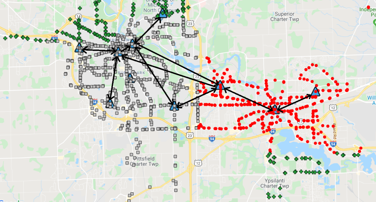
Figure 1: Network Design for the ODMTS with 10 Hubs with $\Delta=2$.

Table 1: Adoption Rates, Average Route Time and Average Ride Cost for the ODMTS.

income level	#trips	%adoption	#riders	%adoption	avg route time (s)	avg route cost ($)
low	476	1.00	877	1.00	901.45	2.41
middle	784	0.96	1615	0.97	553.43	2.43
high	149	0.72	285	0.79	583.10	2.78

Table 1 shows the rider preferences, and the average time and cost of the obtained routes. In particular, columns ‘#trips’ and ‘#riders’ represent the number of trips and riders of the ODMTS. The “%adoption” columns correspond to the adoption rate, i.e., the percentage of trips or riders utilizing the ODMTS. When computing the adoption rate, these numbers include the initial set of riders, i.e., 100% of low-income riders, 75% of middle-income riders and 50% of high-income riders. The cost and convenience of the ODMTS is sufficiently attractive to exhibit significant mode switching, even for the high-income population. Columns for the average route time and cost represent the averages for the obtained routes regardless of the fact that whether riders adopts the transit system or not. The results highlight the high adoption rates. The average route time is the longest for the low-income riders given their long commuting trips. Similar results are observed for the number of transfers, which include the transfers between on-demand shuttles and buses, and between the buses in the hubs. Specifically, from the set of riders choosing the transit system, 22% of low-income riders, 8% of medium-income riders, and 3% of high-income riders have at least 3 transfers. Moreover, the number of transfers decreases with increases in income level.

Table 2: Comparing the Average Cost and Time of the ODMTS trips and those Using Personal Vehicles (Cars).

	ODMTS Trips				Car Trips
	Time		Cost		Time		Cost
income level	ODMTS	Cars	ODMTS	Cars	ODMTS	Cars	ODMTS	Cars
low	901.45	405.96	2.41	10.72	NA		NA
medium	528.94	296.95	2.38	7.14	1489.80	585.03	5.17	14.55
high	529.84	326.53	2.30	7.06	93.77	31.51	0.21	0.88

Table 2 presents a cost and convenience analysis for the ODMTS trips and those using personal vehicles. It also provides the cost and convenience of the other mode, i.e., the convenience and cost of using a personal vehicle for those using the ODMTS and vice-versa. As can be seen, the cost of using the ODMTS is significantly lower, although personal vehicles would decrease the commute time significantly for low-income riders. Note however that the ODMTS has also achieved low commuting times. Riders using personal vehicles do so because the transit times are simply too large for their trips.

Figure 2: Network design for the ODMTS with 10 Hubs with $\Delta=5$.

The next results examine the effect of the threshold value $\Delta$ on the rides with on-demand shuttles. Figure 2 presents the network design with $\Delta=5$ mile. This allows for longer shuttle rides from origin to destination of each trip compared to the $\Delta=2$ case in Figure 1. As a result, the network design has fewer connections between hubs. Although the investment cost for the network design is lower in this case, the average route cost of the obtained trips increases and the average time of the trips decreases through the adoption of more on-demand shuttles. This highlights the trade-off between the high-frequency buses and on-demand shuttles.

6.2 The Benefits of the Formulation

This section compares the novel bilevel formulation with latent demand (L) with the original formulation that ignores the latent demand (O). In other words, the original formulation designs the network with $T\setminus T^{\prime}$ trips but is evaluated on the complete set $T$ of trips. The two network designs are then compared in terms of cost and convenience. To obtain a realistic setting, the share of public transit is assumed to be 10% for each income level. The results are presented in Table 3.

Table 3: Comparison of the Proposed Model (L) and the Original Model (O) with $\Delta=5$.

Model	Income	Adoption	Investment ($)	ODMTS trips ($)	Conv. (s)	Cost & Conv.
L	low	1.00	2482.38	17530.24	1269263.87	32505.13
	middle	1.00
	high	0.84
O	low	1.00	861.54	20685.56	1167457.12	33006.20
	middle	0.99
	high	0.82

The results show that both models have similar results in terms of mode switching. However, the new formulation has a higher investment cost and a lower cost for the ODMTS trips compared to the original formulation. The difference between the models is highlighted in Figure 3, which shows the network designs under the two approaches: The dashed legs represent the design under the original model, and the other legs correspond to the design of the proposed model. This result is intuitive: With more ridership, the ODMTS should open more legs and further reduces congestion. It shows that the novel formulation provides a more robust solution that should reassure transit agencies. As the original formulation opens fewer legs between hubs, users utilize more on-demand shuttles, resulting in trips with more convenience but at much higher costs. In terms of the total investment and trips cost, the results show that the new and original formulations have total costs of $20012.62 and $21547.10, respectively. As this cost improvement corresponds to a planning horizon of 4 hours, it scales up to a gain of $1227585 over a yearly plan with 200 days over 16 hours. This is significant for this case study and highlights why transit agencies are worried about the success of ODMTS when they are planned with the existing demand only: They will under-invest in bus lines and sustain higher shuttle costs. The formulation proposed in this paper remedies this limitation: By taking into account the personalized choice models of riders, the network design invests in high-frequency buses, decreasing the overall cost while maintaining an attractive level of convenience. Note also that, the pricing model adopted in this paper keeps the transit costs low but is also conducive to numerous mode switchings, since the transit system subsidies half the cost.

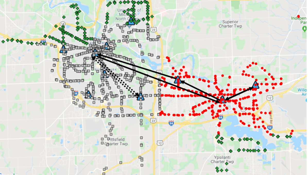
Figure 3: Network Designs of the Proposed Model (L) and the Original Model (O).

It is also important to report the computational performance of the proposed algorithms. The formulation with latent demand requires 513 seconds to converge in 8 iterations, whereas the original formulation requires 189 seconds in 8 iterations for the presented case study.

7 Conclusion

This study presented a bilevel optimization approach for modeling the ODMTS by integrating rider preferences and considering latent demand. The transit network designer optimizes the network design between the hubs for connecting them with high frequency buses, whereas each rider tries to find the most cost-efficient and convenient route under a given design through buses and on-demand shuttles. The paper considered a generic preference model to capture whether riders switch to the ODMTS based on the obtained route and their current mode of travel. To solve the resulting optimization problem, the paper proposed a novel decomposition approach and developed combinatorial Benders cuts for coupling the network design decisions with rider preferences. A cut strengthening was also proposed to exploit the structure of the follower problem and, in particular, a monotonicity assumption of the choice model. The potential of the approach was demonstrated on a case study using a data set from Ann Arbor, Michigan. The results showed that ignoring latent demand can lead to significant cost increase (about 7.5%) for transit agencies, confirming that these agencies are correct in worrying about customer adoption. This is the case even for a pricing model where the transit agency and riders share the shuttle costs. The new formulation can also be solved in reasonable time.

Current work is devoted to examining the impact of various cost models and different choice models for riders. Applications of the model to the city of Atlanta is also contemplated and should reveal some interesting modeling and computational challenges given the size of the city.

Acknowledgements

This research is partly supported by NSF Leap HI proposal NSF-1854684.

References

- [1] Campbell, A.M., Van Woensel, T.: Special issue on recent advances in urban transport and logistics through optimization and analytics. Transportation Science 53(1), 1–5 (2019)
- [2] Campbell, J.F., Ernst, A.T., Krishnamoorthy, M.: Hub arc location problems: Part ii—formulations and optimal algorithms. Management Science 51(10), 1556–1571 (2005)
- [3] Campbell, J.F., Ernst, A.T., Krishnamoorthy, M.: Hub arc location problems: Part i—introduction and results. Management Science 51(10), 1540–1555 (2005)
- [4] Colson, B., Marcotte, P., Savard, G.: Bilevel programming: A survey. 4OR 3(2), 87–107 (2005)
- [5] Farahani, R.Z., Hekmatfar, M., Arabani, A.B., Nikbakhsh, E.: Hub location problems: A review of models, classification, solution techniques, and applications. Computers & Industrial Engineering 64(4), 1096 – 1109 (2013)
- [6] Farahani, R.Z., Miandoabchi, E., Szeto, W., Rashidi, H.: A review of urban transportation network design problems. European Journal of Operational Research 229(2), 281 – 302 (2013)
- [7] Fontaine, P., Minner, S.: Benders decomposition for discrete–continuous linear bilevel problems with application to traffic network design. Transportation Research Part B: Methodological 70, 163 – 172 (2014)
- [8] Laporte, G., Marín, A., Mesa, J.A., Perea, F.: Designing robust rapid transit networks with alternative routes. Journal of Advanced Transportation 45(1), 54–65 (2011)
- [9] LeBlanc, L.J., Boyce, D.E.: A bilevel programming algorithm for exact solution of the network design problem with user-optimal flows. Transportation Research Part B: Methodological 20(3), 259 – 265 (1986)
- [10] Magnanti, T.L., Wong, R.T.: Accelerating benders decomposition: Algorithmic enhancement and model selection criteria. Operations Research 29(3), 464–484 (1981)
- [11] Mahéo, A., Kilby, P., Van Hentenryck, P.: Benders decomposition for the design of a hub and shuttle public transit system. Transportation Science 53(1), 77–88 (2019)
- [12] Sinha, A., Malo, P., Deb, K.: A review on bilevel optimization: From classical to evolutionary approaches and applications. IEEE Transactions on Evolutionary Computation 22(2), 276–295 (2018)
- [13] Van Hentenryck, P.: Social-aware on-demand mobility systems. ISE Magazine (Fall 2019)
- [14] Yu, B., Kong, L., Sun, Y., Yao, B., Gao, Z.: A bi-level programming for bus lane network design. Transportation Research Part C: Emerging Technologies 55, 310 – 327 (2015)
- [15] Zhao, X., Yan, X., Van Hentenryck, P.: Modeling heterogeneity in mode-switching behavior under a mobility-on-demand transit system: An interpretable machine learning approach. CoRR abs/1902.02904 (2019), http://arxiv.org/abs/1902.02904