Finding entries of maximum absolute value in low-rank tensors

Abstract

We present an iterative method for the search of extreme entries in low-rank tensors which is based on a power iteration combined with a binary search. In this work we use the HT-format for low-rank tensors but other low-rank formats can be used verbatim. We present two different approaches to accelerate the basic power iteration: an orthogonal projection of Rayleigh-Ritz type, as well as an acceleration of the power iteration itself which can be achieved due to the diagonal structure of the underlying eigenvalue problem. Finally the maximizing index is determined by a binary search based on the proposed iterative method for the approximation of the maximum norm. The iterative method for the maximum norm estimation inherits the linear complexity of the involved tensor arithmetic in the HT-format w.r.t. the tensor order, which is also verified by numerical tests.

1 Introduction

Scientific computing with functions, vectors and matrices in low rank formats allows us to tackle even high-dimensional and extreme scale problems, provided the underlying mathematical objects allow for a low rank approximation. In this article we focus on the task of postprocessing low rank matrices and tensors. Our guiding problem is to find the entry of maximum absolute value in a low rank object without accessing every entry. Such a task is the discrete analogue to finding global optima and thus of general interest. While this is straight-forward for rank one, it is surprisingly difficult for ranks beyond one. The seminal idea for finding the maximum absolute value efficiently stems from the PhD thesis of Mike Espig [5] where the problem is reformulated as a diagonal (extreme scale) eigenvalue problem. The latter can e.g. be solved by a simple power iteration, and in case that there is a unique maximizer, the corresponding eigenvector is rank one. Hence, it makes sense to approximate the eigenvector by low rank (cf. [6] for a recent approach independently of this article). However, if several entries are of similar size, then the power iteration can be arbitrarily slow, the iterates cannot be approximated by low rank and a truncation to low rank may destroy convergence altogether.

In this article we provide much more advanced approaches for finding the maximum by subspace acceleration and a squaring trick. Without truncation we are able to prove a uniformly good convergence rate of $1/2$ for computing the $\|\cdot\|_{\infty}$-norm and based on this we devise a divide and conquer strategy to find the corresponding entry.

The article is structured as follows: In Section 2 we introduce the HT-format followed by the problem for rank one or elementary tensors in Section 3. In Section 4 we summarize the power iteration approach and give examples that underline the involved difficulties. In Section 5 we provide the subspace acceleration and in Section 6 the squaring trick. Finally, in Section 7 we explain how one can determine the entry of maximum absolute value based on the so far introduced iterative methods. We conclude by giving numerical examples in Section 8 that show the benefits and limitations of the algorithms.

2 Low-rank formats for tensors

We denote the entry of an order $d$ tensor $\mathbf{a}\in\mathbb{R}^{I},I=\bigtimes_{\mu=1}^{d}I_{\mu}$, by

$$\mathbf{a}[\mathbf{i}]=\mathbf{a}[i_{1},\ldots,i_{d}]\;,\qquad\mathbf{i}=(i_{1},\ldots,i_{d})\in I.$$

For larger tensor order $d\gg 2$ a full (entrywise) representation is not feasible (cf. the curse of dimensionality [3, 2]) and additional structure is required. In the following we use low rank tensors that generalize the matrix rank.

Definition 1 (Elementary tensors).

A tensor $\mathbf{a}\in\mathbb{R}^{I}$ is called elementary tensor or rank $1$ tensor if

$$\mathbf{a}=\bigotimes_{\mu=1}^{d}u^{(\mu)}=u^{(1)}\otimes\cdots\otimes u^{(d)},\qquad u^{(\mu)}\in\mathbb{R}^{I_{\mu}},\quad\mu=1,\ldots,d.$$ (1)

The CP-rank (Canonical Polyadic) [14] of a tensor $\mathbf{a}\in\mathbb{R}^{I}$ is defined as the minimum number $\mathrm{rank}(a)=r\in\mathbb{N}_{0}$ such that

$$\mathbf{a}=\sum_{k=1}^{r}U^{(1)}[\bullet,k]\otimes\cdots\otimes U^{(d)}[\bullet,k],\qquad U^{(\mu)}\in\mathbb{R}^{I_{\mu}\times r},\quad\mu=1,\ldots,d.$$ (2)

For computational purposes the minimum number $r$ of terms is not necessary, instead any representation of the form (2) with reasonably small $r$ is sufficient. Such a representation is called CP-format with representation rank $r$. The corresponding set is defined by

$$\mathcal{R}_{r}:=\{\mathbf{a}\in\mathbb{R}^{I}\;:\;\mathop{\operator@font rank}\nolimits(\mathbf{a})\leq r\}.$$ (3)

These sets are numerically difficult and thus a different type of rank is commonly used which is based on matricizations.

Definition 2 ($t$-matricization).

Let $\mathbf{a}\in\mathbb{R}^{I}$. We denote

$$I_{t}:=\bigtimes_{\mu\in t}I_{\mu}\qquad\mbox{and}\qquad I_{[t]}:=\bigtimes_{\mu\notin t}I_{\mu},\qquad t\subseteq\{1,\ldots,d\}$$ (4)

and we use the short notation

$$\mathbf{i}_{t}=(i_{\mu})_{\mu\in t},i_{t}\in I_{t}\qquad\mathbf{i}_{[t]}=(i_{\mu})_{\mu\notin t},i_{[t]}\in I_{[t]}.$$ (5)

Then the $t$-matricization $\mathcal{M}_{t}(\mathbf{a})\in\mathbb{R}^{I_{t}\times I_{[t]}}$ of $\mathbf{a}$ is defined by

$$\mathcal{M}_{t}(\mathbf{a})[\mathbf{i}_{t},\,\mathbf{i}_{[t]}]:=\mathbf{a}[\mathbf{i}],\qquad\mathbf{i}=(i_{1},\ldots,i_{d})\in I,$$

i.e. a rearrangement of $\mathbf{a}$ into a matrix with row index set $I_{t}$ and column index set $I_{[t]}$.

For the CP-format, instead of all tensor entries $\mathbf{a}[i_{1},\ldots,i_{d}]$ of some tensor $\mathbf{a}\in\mathbb{R}^{I}$, the matrices $U^{(\mu)}\in\mathbb{R}^{I_{\mu}\times r}$ from the right-hand side of (2) are stored. Assuming all tensor directions to be of the same size $n=\#I_{\mu}$, this sums up to a storage complexity of $dnr$, which is linear in the tensor order $d$. Despite of this desirable linear complexity in $d$, the CP-format has two drawbacks: on the one hand, the CP-rank is in general NP-hard to determine, cf. [15], on the other hand, the set (3) is not closed for tensors of higher order $d\geq 3$, cf. [4, 12]. This fact can render the numerical treatment of tensors in CP-format difficult.

For the Tucker format the corresponding set is closed, cf. [12], but the storage complexity w.r.t. the tensor order $d$ is exponential.

The above mentioned complexities and shortcomings transfer to many arithmetic operations, such as dot products or Hadamard products, which are involved in the algorithms presented in this article. All of the shortcomings can be resolved by using the Hierarchical Tucker format (HT-format) introduced in the following.

2.1 The Hierarchical Tucker format

An HT-format for a tensor $\mathbf{a}\in\mathbb{R}^{I}$, $I=\bigtimes_{\mu=1}^{d}I_{\mu}$, is based on a hierarchy of all tensor directions $D:=\{1,\ldots,d\}$, which can be expressed by a binary tree, referred to as dimension tree, cf. [8, 12]:

Definition 3 (Dimension tree).

For a tensor space $\mathbb{R}^{I}$, $I=\bigtimes_{\mu=1}^{d}I_{\mu}$, by $D=\{1,\ldots,d\}$ we denote the set of all tensor directions. A corresponding dimension tree $T_{D}$ is a tree with the following properties:

1. all vertices of $T_{D}$ are non-empty subsets of $D$,

2. the root vertex of $T_{D}$ is the set $D$: $\operatorname{root}(T_{D})=D$,

3. all vertices $t\in T_{D}$ with $\#t>1$ have two disjoint successors $\operatorname{sons}(t)=\{s_{1},s_{2}\}$ with

   $$t=s_{1}\dot{\cup}s_{2}\qquad\mbox{(disjoint union)}.$$

A dimension tree $T_{D}$ for a tensor order $d\in\mathbb{N}$, $D=\{1,\ldots,d\}$, is thus a binary tree with singletons $\{\mu\}$, $\mu=1,\ldots,d$, at the leaf vertices. Two examples of dimension trees for tensor order $d=4$ are shown in Figure 1.

[.$\{1,2,3,4\}$ [.$\{1,2\}$ $\{1\}$ $\{2\}$ ].$\{1,2\}$ [.$\{3,4\}$ $\{3\}$ $\{4\}$ ].$\{3,4\}$ ].$\{1,2,3,4\}$

[.$\{1,2,3,4\}$ $\{1\}$ [.$\{2,3,4\}$ $\{2\}$ [.$\{3,4\}$ $\{3\}$ $\{4\}$ ].$\{3,4\}$ ].$\{2,3,4\}$ ].$\{1,2,3,4\}$

Figure 1: Two different dimension trees for tensor order $d=4$.

The HT-format is again defined by matricizations, cf. Definition 2, where the subsets $t\subseteq\{1,\ldots,d\}$ are the subsets $t\in T_{D}$ of the underlying dimension tree $T_{D}$ which determines the structure of the HT-format:

Definition 4 (Hierarchical Tucker format (HT-format)).

Let $\mathbf{a}\in\mathbb{R}^{I}$, $I=\bigtimes_{\mu=1}^{d}I_{\mu}$, be a tensor and $T_{D}$, $D=\{1,\ldots,d\}$, a dimension tree. Furthermore, for all $t\in T_{D}$ let

$$\mathcal{M}_{t}(\mathbf{a})=U^{(t)}(V^{(t)})^{\top},\qquad U^{(t)}\in\mathbb{R}^{I_{t}\times r_{t}},\qquad V^{(t)}\in\mathbb{R}^{I_{[t]}\times r_{t}},$$ (6)

$I_{t}$, $I_{[t]}$ as in (4), be a decomposition of the $t$-matricization of $\mathbf{a}$, where the $U^{(t)}$, $t\in T_{D}$, are referred to as frames: the columns of $U^{(t)}$ span the range of $\mathcal{M}_{t}(\mathbf{a})$, especially for $t=D$ we assume (6) to be chosen such that

$$\mathbf{a}=\mathcal{M}_{D}(\mathbf{a})=U^{(D)}$$ (7)

holds, i.e. $V^{(D)}=1\in\mathbb{R}^{1\times 1}$. A Hierarchical Tucker format (HT-format) for $\mathbf{a}$ is then defined by

1. the above matrices $U^{(\{\mu\})}\in\mathbb{R}^{I_{\mu}\times r_{\{\mu\}}}$ for all leaf vertices $\{\mu\}$, $\mu=1,\ldots,d$, of $T_{D}$ and

2. transfer tensors $\mathbf{b}^{(t)}\in\mathbb{R}^{r_{t}\times r_{s_{1}}\times r_{s_{2}}}$ at all non-leaf vertices $t\in T_{D}$, $\operatorname{sons}(t)=\{s_{1},s_{2}\}$, with $r_{D}=1$ at the root, which fulfill for all $k=1,\ldots,r_{t},$

   $$U^{(t)}[\bullet,k]=\sum_{k_{1}=1}^{r_{s_{1}}}\sum_{k_{2}=1}^{r_{s_{2}}}\mathbf{b}^{(t)}[k,k_{1},k_{2}]U^{(s_{1})}[\bullet,k_{1}]\otimes U^{(s_{2})}[\bullet,k_{2}],$$ (8)

   i.e. the transfer tensor $\mathbf{b}^{(t)}$ holds the coefficients of the linear combination (8) by which the frame $U^{(t)}$ can be obtained from the frames $U^{(s_{1})}$ and $U^{(s_{2})}$.

The vector $\mathbf{r}=(r_{t})_{t\in T_{D}}$ containing the numbers of columns of the frames $U^{(t)}$, $t\in T_{D}$, is called representation rank of the HT-format. Notice that we always assume $r_{D}=1$ at the root, i.e. $U^{(D)}$ contains only one column, namely $\mathcal{M}_{D}(\mathbf{a})=\mathbf{a}$, cf. (7).

Definition 5 (Hierarchical Tucker rank (HT-rank)).

The Hierarchical Tucker rank (HT-rank) of a tensor $\mathbf{a}\in\mathbb{R}^{I}$, $I=\bigtimes_{\mu=1}^{d}I_{\mu}$, w.r.t. some dimension tree $T_{D}$, $D=\{1,\ldots,d\}$, is defined as the vector $\mathbf{r}=(r_{t})_{t\in T_{D}}$ containing the smallest possible numbers $r_{t}$, $t\in T_{D}$, such that an HT-format of $\mathbf{a}$ with representation rank $\mathbf{r}$ exists.

Notice that by (6) the components $r_{t}$, $t\in T_{D}$, of the HT-rank of $\mathbf{a}\in\mathbb{R}^{I}$, $I=\bigtimes_{\mu=1}^{d}I_{\mu}$, w.r.t to some dimension tree $T_{D}$ are the ranks of the respective matricizations $\mathcal{M}_{t}(\mathbf{a})\in\mathbb{R}^{I_{t}\times I_{[t]}}$, denoted as

$$\mathop{\operator@font rank}\nolimits_{t}(\mathbf{a}):=\mathop{\operator@font rank}\nolimits(\mathcal{M}_{t}(\mathbf{a})).$$

According to (3) for $\mathbf{r}\in\mathbb{N}_{0}^{T_{D}}$, $r_{D}=1$, we define the set $\mathcal{H}_{\mathbf{r}}$ as

$$\mathcal{H}_{\mathbf{r}}:=\{\mathbf{a}\in\mathbb{R}^{I}\;:\;\mathop{\operator@font rank}\nolimits_{t}(\mathbf{a})\leq r_{t},\;t\in T_{D}\},$$ (9)

i.e. the set of all tensors for which an HT-representation with representation rank $\mathbf{r}$ exists. It can be shown that $\mathcal{H}_{\mathbf{r}}$ is a closed subset of $\mathbb{R}^{I}$, cf. [12].

Evaluation of tensor entries

Let $\mathbf{a}\in\mathbb{R}^{I}$, $I=\bigtimes_{\mu=1}^{d}I_{\mu}$, be represented in the HT-format w.r.t. some dimension tree $T_{D}$, i.e. at the leaf vertices $\{\mu\}\in T_{D}$ the matrices $U^{(\{\mu\})}\in\mathbb{R}^{I_{\mu}\times r_{\{\mu\}}}$ are stored and at the non-leaf vertices $t\in T_{D}$ the transfer tensors $\mathbf{b}^{(t)}\in\mathbb{R}^{r_{t}\times r_{s_{1}}\times r_{s_{1}}}$, $\operatorname{sons}(t)=\{s_{1},s_{2}\}$, are stored. The tensor entries $\mathbf{a}[\mathbf{i}]$, $\mathbf{i}=(i_{1},\ldots,i_{d})\in I$, are thus not available explicitly but can be computed recursively: by (7) we have

$$\mathbf{a}[\mathbf{i}]=U^{(D)}[\mathbf{i}],$$

which can be evaluated by using (8):

$$U^{(D)}[\mathbf{i}]\underset{\eqref{equation:htNestedness}}{=}\sum_{k_{1}=1}^{r_{t_{1}}}\sum_{k_{2}=1}^{r_{t_{2}}}\mathbf{b}^{(D)}[k_{1},k_{2}]U^{(t_{1})}[\mathbf{i}_{t_{1}},k_{1}]U^{(t_{2})}[\mathbf{i}_{t_{2}},k_{2}],\quad\operatorname{sons}(D)=\{t_{1},t_{2}\},$$ (10)

where we use the notation (5) for sub-indices of $\mathbf{i}\in I$ corresponding to some subset $t\subseteq\{1,\ldots,d\}$. The columns $U^{(t_{1})}[\bullet,k_{1}]$ and $U^{(t_{2})}[\bullet,k_{2}]$ are either stored explicitly (if the corresponding vertex $t_{1}$ or $t_{2}$ is a leaf of $T_{D}$) or can again be evaluated recursively by using (8). By this means, the tensor entries $\mathbf{a}[\mathbf{i}]$, $\mathbf{i}\in I$, of $\mathbf{a}$ can be evaluated with a computational work growing like $\mathcal{O}(dr^{3})$, i.e. linearly with the tensor order $d$, when $r\in\mathbb{N}$ is an upper bound for the components of the representation rank $\mathbf{r}=(r_{t})_{t\in T_{D}}$.

Storage complexity

The storage complexity for a tensor $\mathbf{a}\in\mathbb{R}^{I}$, $I=\bigtimes_{\mu=1}^{d}I_{\mu}$, in HT-representation w.r.t. some dimension tree $T_{D}$ also grows linearly with the tensor order $d$ (as for the CP-format): assuming all tensor directions to be of the same size $n=\#I_{\mu}$ and a bound $r\in\mathbb{N}$ for the components of the representation rank $\mathbf{r}=(r_{t})_{t\in T_{D}}$ of $\mathbf{a}$, $nr$ real numbers have to be stored at each leaf vertex $\{\mu\}\in T_{D}$, $\mu=1,\ldots,d$, cf. Definition 4 (a), and $r^{3}$ real numbers have to be stored at each interior vertex (neither leaf nor root) and $r^{2}$ real numbers at the root. Taking into account that a dimension tree $T_{D}$, $D=\{1,\ldots,d\}$, consists of $d$ leaf vertices and $d-1$ non-leaf vertices, this sums up to a storage complexity of $\mathcal{O}(d(nr+r^{3}))$.

Arithmetic operations in the HT-format

Two arithmetic operations for tensors, which are of particular importance for this article, are the dot product $\langle\mathbf{x},\mathbf{y}\rangle\in\mathbb{R}$ and the Hadamard product $\mathbf{x}\circ\mathbf{y}\in\mathbb{R}^{I}$ of two tensors $\mathbf{x},\mathbf{y}\in\mathbb{R}^{I}$, defined by

$$\langle\mathbf{x},\mathbf{y}\rangle:=\sum_{\mathbf{i}\in I}\mathbf{x}[\mathbf{i}]\cdot\mathbf{y}[\mathbf{i}],\qquad(\mathbf{x}\circ\mathbf{y})[\mathbf{i}]:=\mathbf{x}[\mathbf{i}]\mathbf{\cdot}\mathbf{y}[\mathbf{i}],\quad\mathbf{i}\in I.$$

These operations can be computed directly in the HT-format, cf. [12, 11]. The corresponding complexities grow again linearly with the tensor order $d$: assuming all tensor directions to be of the same size $n\in\mathbb{N}$ and an upper bound $r\in\mathbb{N}$ for the components of the representation ranks of $\mathbf{x}$ and $\mathbf{y}$, dot products can be computed with a complexity bounded by $\mathcal{O}(d(nr^{2}+r^{4}))$ flops whereas $\mathcal{O}(d(nr^{2}+r^{6}))$ flops are needed for the computation of Hadamard products (cf. [11] for a parallel algorithm).

A more detailed description of different low-rank formats for tensors can e.g. be found in [12, 10]. For this article we use the HT-format but other formats can be used as well, e.g. the TT-format [20, 12] or MPS format [21, 22]. Since the computation of the Hadamard product of two low-rank tensors typically yields a result of higher representation rank, one needs a truncation procedure which truncates tensors back to lower ranks. For the HT-format we use the truncation techniques introduced in [8] the complexity of which is comparable to that of the computation of dot products above.

3 Maximum entries of elementary tensors

Let $\mathbf{a}\in\mathbb{R}^{I}$, $I=\bigtimes_{\mu=1}^{d}I_{\mu}$.

Definition 6 (Maximum norm of a tensor).

The maximum norm of a tensor $\mathbf{a}$ is defined by $\|\mathbf{a}\|_{\infty}:=\max\{|\mathbf{a}[\mathbf{i}]|\;:\;\mathbf{i}\in I\}$.

Maximum norm of a matrix

Notice that Definition 6 may lead to an ambiguity: for a matrix $M\in\mathbb{R}^{m\times n}$, $\|M\|_{\infty}$ is often used to denote the operator norm $\|M\|_{\mathrm{op},\infty}$ of $M$ as a linear operator $(\mathbb{R}^{n},\|\cdot\|_{\infty})\to(\mathbb{R}^{m},\|\cdot\|_{\infty})$ which does not match Definition 6:

$$\|M\|_{\mathrm{op},\infty}:=\sup_{\|x\|_{\infty}=1}\|Mx\|_{\infty}=\max_{i=1,\ldots,m}\|M[i,\bullet]\|_{1},$$

cf. [7], where $M[i,\bullet]$ denotes the $i$-th row of $M$. In the following $\|M\|_{\infty}$ is always used according to Definition 6, i.e. $\|M\|_{\infty}=\max\{|M[i,j]|\;:\;i=1,\ldots,m,\;j=1,\ldots,n\}$.

Maximum norm of an elementary tensor

Let $\mathbf{a}=u^{(1)}\otimes\cdots\otimes u^{(d)}$, $u^{(\mu)}\in\mathbb{R}^{I_{\mu}}$, $\mu=1,\ldots,d$, be an elementary tensor. The maximum norm of $\mathbf{a}$ is then given by

$$\|\mathbf{a}\|_{\infty}=\max_{\mathbf{i}\in I}|a[\mathbf{i}]|=\prod_{\mu=1}^{d}|u^{(\mu)}[\bullet]|_{\infty},$$

which can be maximized by maximizing each of the factors $|u^{(\mu)}[\bullet]|$, $\mu=1,\ldots,d$, in complexity ${\cal O}(dn)$. Unfortunately, no such algorithm is known for tensors of higher rank (i.e. non-elementary tensors). Even if a good approximation of a matrix $M$ by a rank-$1$ matrix $\tilde{M}$ exists in the Euclidean sense (e.g. a truncated singular value decomposition), the corresponding maximum norms $\|M\|_{\infty}$ and $\|\tilde{M}\|_{\infty}$ may differ extremely as the following example indicates:

Example

Consider a matrix $M\in\mathbb{R}^{n\times n}$ defined as

$$M:=\underbrace{\frac{\sigma_{1}}{n-1}\left(\begin{array}[]{r|rrr}0&&&\\ \hline\cr&1&\cdots&1\\ &\vdots&\ddots&\vdots\\ &1&\cdots&1\end{array}\right)}_{M_{1}}+\underbrace{\sigma_{2}\left(\begin{array}[]{r|rrr}1&&&\\ \hline\cr&0&\cdots&0\\ &\vdots&\ddots&\vdots\\ &0&\cdots&0\end{array}\right)}_{M_{2}},\qquad\sigma_{1}>\sigma_{2}\geq 0.$$ (11)

Then $M$ has the singular values $\sigma_{1}>\sigma_{2}$ and $M_{1}$ is the rank-$1$ best approximation of $M$ in the Frobenius (and spectral) norm with an approximation error

$$\frac{\|M-M_{1}\|_{F}}{\|M\|_{F}}=\sqrt{\frac{\sigma_{2}^{2}}{\sigma_{1}^{2}+\sigma_{2}^{2}}}\leq\frac{\sigma_{2}}{\sigma_{1}}$$ (12)

in the Frobenius norm. Assuming $\sigma_{2}>\frac{\sigma_{1}}{n-1}$ we get a corresponding error

$$\frac{|\|M\|_{\infty}-\|M_{1}\|_{\infty}|}{\|M\|_{\infty}}=\frac{\sigma_{2}-\frac{\sigma_{1}}{n-1}}{\sigma_{2}}=1-\frac{\sigma_{1}}{\sigma_{2}}\cdot\frac{1}{n-1}$$ (13)

for the approximation of the maximum norm, which tends to $1$ for $n\to\infty$, independently of the error (12).

4 Estimating the maximum norm by a power iteration

We use a power iteration to approximate the maximum norm $\|\mathbf{a}\|_{\infty}$ of a tensor $\mathbf{a}\in\mathbb{R}^{I}$, $I=\bigtimes_{\mu=1}^{d}I_{\mu}$, as introduced in [5]: consider the diagonal matrix

$$D\in\mathbb{R}^{I\times I},\qquad\mathop{\operator@font diag}\nolimits(D)=\mathbf{a}.$$ (14)

Then the maximum norm $\|\mathbf{a}\|_{\infty}$ is the maximum absolute value of an eigenvalue of $D$:

$$\|\mathbf{a}\|_{\infty}=\max\{|\lambda|\;:\;D\mathbf{v}=\lambda\mathbf{v}\;\mbox{for some}\;\mathbf{v}\neq\mathbf{0}\},$$ (15)

which can be computed by a standard power iteration if there exists only one eigenvalue $\lambda$ of $D$ with $|\lambda|=\|\mathbf{a}\|_{\infty}$, i.e. there is only one index $\mathbf{i}\in I$ with $\|\mathbf{a}\|_{\infty}=|\mathbf{a}[\mathbf{i}]|$. Taking into account that the matrix multiplication $D\mathbf{v}$, $\mathbf{v}\in\mathbb{R}^{I}$, can be written as the Hadamard product $\mathbf{a}\circ\mathbf{v}$, this results in Algorithm 1, where $\|\mathbf{a}\|=\|\mathbf{a}\|_{2}$ denotes the Euclidean norm of $\mathbf{a}$.

1$\mathbf{a}^{(1)}:=\mathbf{a}/\|\mathbf{a}\|$;

2 for  $j=1,2,\ldots$  do

3       $\mathbf{a}^{(j+1)}:=\mathbf{a}\circ\mathbf{a}^{(j)}$;

       $\lambda^{(j+1)}:=\langle\mathbf{a}^{(j)},\mathbf{a}^{(j+1)}\rangle$ // Rayleigh quotient

4       $\mathbf{a}^{(j+1)}\leftarrow\mathbf{a}^{(j+1)}/\|\mathbf{a}^{(j+1)}\|$;

5      

Algorithm 1 Power iteration: the maximum norm $\|\mathbf{a}\|_{\infty}$ of a tensor $\mathbf{a}\in\mathbb{R}^{I}$, $I=\bigtimes_{\mu=1}^{d}I_{\mu}$, is approximated by $|\lambda^{(j+1)}|$, $j\in\mathbb{N}$, if only one index $\mathbf{i}\in I$ with $\|\mathbf{a}\|_{\infty}=|\mathbf{a}[\mathbf{i}]|$ exists.

Improvement of the Rayleigh quotient

Due to the diagonal structure of the eigenvalue problem in (15), the Rayleigh quotient in line 1 of Algorithm 1 can be improved, which results in a new estimator $\alpha^{(j+1)}:=\|\mathbf{a}^{(j+1)}\|$, $j\in\mathbb{N}$, cf. Algorithm 2.

Lemma 7 (Improved estimator for the power iteration).

The new estimator $\alpha^{(j+1)}$, $j\in\mathbb{N}$, of Algorithm 2 is at least as good as the Rayleigh quotient $\lambda^{(j+1)}$, $j\in\mathbb{N}$, from the standard power iteration, cf. Algorithm 1:

$$|\lambda^{(j+1)}|\leq\alpha^{(j+1)},\qquad j\in\mathbb{N},$$ (16)

and always converges to $\|\mathbf{a}\|_{\infty}$ from below: $\alpha^{(j+1)}\uparrow\|\mathbf{a}\|_{\infty}$, $j\to\infty$.

Proof.

Using the Cauchy-Schwarz inequality and $\|\mathbf{a}^{(j)}\|=1$ in line 1 of Algorithm 1 yields

$$|\lambda^{(j+1)}|=|\langle\mathbf{a}^{(j)},\mathbf{a}^{(j+1)}\rangle|\leq\|\mathbf{a}^{(j)}\|\|\mathbf{a}^{(j+1)}\|=\|\mathbf{a}^{(j+1)}\|=\alpha^{(j+1)},$$

i.e. (16). By induction one easily verifies that $\mathbf{a}^{(j)}=\mathbf{a}^{\circ j}/\|\mathbf{a}^{\circ j}\|$, $j\in\mathbb{N}$, holds in line 2 of Algorithm 2, where $\mathbf{a}^{\circ j}$ denotes the $j$-fold Hadamard product of $\mathbf{a}$. This implies

$$\alpha^{(j+1)}=\|\mathbf{a}\circ\mathbf{a}^{(j)}\|=\frac{\|\mathbf{a}\circ\mathbf{a}^{\circ j}\|}{\|\mathbf{a}^{\circ j}\|}\leq\frac{\|\mathbf{a}\|_{\infty}\|\mathbf{a}^{\circ j}\|}{\|\mathbf{a}^{\circ j}\|}=\|\mathbf{a}\|_{\infty},$$ (17)

in line 2, i.e. $\alpha^{(j+1)}$, $j\in\mathbb{N}$, are lower bounds of $\|\mathbf{a}\|_{\infty}$. We now use

$$\|\mathbf{a}^{\circ j}\|=\left(\sum_{\mathbf{i}\in I}\mathbf{a}[\mathbf{i}]^{2j}\right)^{1/2}=\left(\left(\sum_{\mathbf{i}\in I}\mathbf{a}[\mathbf{i}]^{2j}\right)^{1/2j}\right)^{j}=\|\mathbf{a}\|_{2j}^{j}$$ (18)

and the norm equivalence for $p$-norms on $\mathbb{R}^{I}$ which follows from the Hölder inequality:

$$\|\mathbf{a}\|_{2j}\leq N^{\frac{1}{2j}-\frac{1}{2(j+1)}}\|\mathbf{a}\|_{2(j+1)}=N^{\frac{1}{2j(j+1)}}\|\mathbf{a}\|_{2(j+1)},\qquad N=\#I,$$ (19)

as well as

$$\|\mathbf{a}\|_{\infty}\leq\|\mathbf{a}\|_{2(j+1)},$$ (20)

in order to get a lower bound for $\alpha^{(j+1)}$, $j\in\mathbb{N}$:

$$\alpha^{(j+1)} \underset{\eqref{equation:alphajLowerBound}}{=}\frac{\|\mathbf{a}\circ\mathbf{a}^{\circ j}\|}{\|\mathbf{a}^{\circ j}\|}=\frac{\|\mathbf{a}^{\circ(j+1)}\|}{\|\mathbf{a}^{\circ j}\|}\underset{\eqref{equation:powerNorm}}{=}\frac{\|\mathbf{a}\|_{2(j+1)}^{j+1}}{\|\mathbf{a}\|_{2j}^{j}}\underset{\eqref{equation:normEquivalence}}{\geq}\frac{\|\mathbf{a}\|_{2(j+1)}^{j+1}}{N^{1/(2(j+1))}\|\mathbf{a}\|_{2(j+1)}^{j}}$$

$$=N^{-\frac{1}{2(j+1)}}\|\mathbf{a}\|_{2(j+1)}\underset{\eqref{equation:inequalityMaxNormPNorm}}{\geq}N^{-\frac{1}{2(j+1)}}\|\mathbf{a}\|_{\infty}.$$ (21)

Combining the bounds (17) and (21) for $\alpha^{(j+1)}$ yields

$$0\leq\|\mathbf{a}\|_{\infty}-\alpha^{(j+1)}\leq(1-N^{-\frac{1}{2(j+1)}})\|\mathbf{a}\|_{\infty},$$ (22)

i.e. $\alpha^{(j+1)}\uparrow\|\mathbf{a}\|_{\infty}$ for $j\to\infty$ since $1-N^{-\frac{1}{2(j+1)}}\to 0$, $j\to\infty$. ∎

1$\mathbf{a}^{(1)}:=\mathbf{a}/\|\mathbf{a}\|$;

2 for  $j=1,2,\ldots$  do

3       $\mathbf{a}^{(j+1)}:=\mathbf{a}\circ\mathbf{a}^{(j)}$;

       $\alpha^{(j+1)}:=\|\mathbf{a}^{(j+1)}\|$ // improved estimator

4       $\mathbf{a}^{(j+1)}\leftarrow\mathbf{a}^{(j+1)}/\|\mathbf{a}^{(j+1)}\|$;

5      

Algorithm 2 Power iteration: $\alpha^{(j+1)}\uparrow\|\mathbf{a}\|_{\infty}$ for $j\to\infty$, where $\alpha^{(j+1)}$ is bounded from below by the absolute value $|\lambda^{(j+1)}|$ of the Rayleigh quotient from Algorithm 1, cf. Lemma 7.

The following example shows that the estimator $\alpha^{(j+1)}$ from Algorithm 2 is indeed better than the Rayleigh quotient from the standard power iteration:

Example

For the vector (order-$1$ tensor) $\mathbf{a}=[1,-1]\in\mathbb{R}^{2}$ the standard power iteration from Algorithm 1 does not converge to $\|\mathbf{a}\|_{\infty}$:

$$\lambda^{(j+1)}=0,\qquad j\in\mathbb{N}.$$

The estimator $\alpha^{(j+1)}$ from Algorithm 2, however, immediately converges to $\|\mathbf{a}\|_{\infty}$:

$$\alpha^{(j+1)}=1=\|\mathbf{a}\|_{\infty},\qquad j\in\mathbb{N}.$$

Error estimator for Algorithm 2

Since Algorithm 2 is a power iteration for $\mathbf{a}\in\mathbb{R}^{I}$ with an improved estimator for the eigenvalue, cf. Lemma 7, any error estimator known for the standard power iteration can also be applied to Algorithm 2. Since in our framework the underlying matrix is diagonal, cf. (14), results for power iteration with symmetric matrices may be applied. E.g. in [18] the error ${\varepsilon^{(j+1)}:=(\|\mathbf{a}\|_{\infty}-\alpha^{(j+1)})/\|\mathbf{a}\|_{\infty}}$, $j\in\mathbb{N}$, is proven to be bounded by

$$\frac{\ln(N)}{j-1},\quad j\geq 2,\quad N=\#I,$$ (23)

if the corresponding matrix is symmetric positive definite, which in our framework means that all entries of $\mathbf{a}$ are positive, cf. (14).

However, for our special case of a power iteration on a diagonal matrix $D$, the bound

$$\varepsilon^{(j+1)}\leq 1-N^{-\frac{1}{2(j+1)}}$$ (24)

can directly be obtained from (22) in the proof of Lemma 7. Asymptotically the bounds (23) and (24) show the same behavior, where the bound in (24) is always better than the one in (23). Assuming an error which grows like the bound (23) leads to a slow convergence:

$$\varepsilon^{(j+1)}\approx\left(1-\frac{1}{j-1}\right)\varepsilon^{(j)}.$$ (25)

Even though the above error estimates may be pessimistic in some cases, our experiments show that the convergence behavior (25) in fact occurs for many standard examples, cf. Figures 2(a) and 3(a).

Complexity of the power iteration

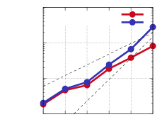
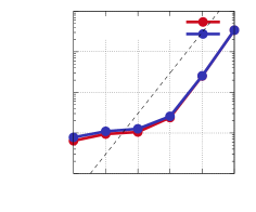
In the HT-format all tensor operations involved in Algorithm 2 can be carried out directly in the HT-format with a complexity depending linearly on the tensor order $d$ and the mode sizes. We can thus expect such a linear complexity for the approximation of $\|\mathbf{a}\|_{\infty}$ by Algorithm 2 with $\mathbf{a}\in\mathbb{R}^{I}$, $I=\bigtimes_{\mu=1}^{d}I_{\mu}$, in HT-representation, which is verified by the experiments in Section 8.6, cf. Figure 7.

Truncation

Since the computation of Hadamard products increases the representation ranks of the iterates, we include truncations in each step of Algorithm 2 in order to keep the representation ranks of the iterates small enough. We compute the truncations by a hierarchical singular value decomposition (HSVD) in the HT-format [8]. A detailed analysis of truncations in iterative fixed-point like processes is given by [13]: if the truncation errors are small enough and the starting tensor is chosen appropriately, the iterative process still converges to the original fixed point, provided that the latter allows for a respective low-rank representation. In our numerical experiments, cf. Section 8, we truncate w.r.t. fixed prescribed HT-ranks in each step of the algorithms, which already worked well. Another option would be to truncate w.r.t. a given tolerance $\varepsilon>0$ for the relative truncation error, which, however, may lead to high representation ranks in the beginning of the algorithms, since the underlying error estimations for the HT-format can be rather pessimistic, cf. [8].

Notice that it is possible to construct counterexamples where any truncation leads to the loss of that entry of $\mathbf{a}\in\mathbb{R}^{I}$ which corresponds to $\|\mathbf{a}\|_{\infty}$, i.e. to a wrong approximation of $\|\mathbf{a}\|_{\infty}$ in the end. Such counterexamples can be constructed as in (11): take $\mathbf{a}=M$ (order-$2$ tensor) as defined in (11) with $\sigma_{1}=(n-1)\varepsilon$ and $\sigma_{2}=1$, $1/(n-1)<\varepsilon<1$. A rank-$1$ best approximation of $M$ is given by $M_{1}$, cf. (11), i.e. after truncation, instead of $\|M\|_{\infty}=1$, the maximum norm $\|M_{1}\|_{\infty}=\varepsilon$ would be computed. This example shows that it may happen that a single entry of larger absolute value (the entry $1$ of $M$) is ”hidden” by many entries of smaller absolute value (the entries $\varepsilon$ of $M$). The reason for this is that the truncation, cf. [8], is based on the singular value decomposition, which corresponds to a best approximation in the Euclidean sense and not w.r.t. the maximum norm. Nevertheless this does not stand in contradiction to the convergence analysis developed in [13] since the truncation of $M$ does not meet the underlying assumptions: the starting tensor $\mathbf{a}/\|\mathbf{a}\|=M/\|M\|_{F}$ of the iterative process is far away from the fixed point $M_{2}$ ($\|M_{2}\|_{F}=1$), cf. (11):

$$\left\|\frac{M}{\|M\|_{F}}-M_{2}\right\|_{F} =\sqrt{\frac{\bigl{(}1-\sqrt{(n-1)^{2}\varepsilon^{2}+1}\bigr{)}^{2}+(n-1)^{2}\varepsilon^{2}}{(n-1)^{2}\varepsilon^{2}+1}}$$

$$\geq\sqrt{\frac{(n-1)^{2}\varepsilon^{2}}{1+(n-1)^{2}\varepsilon^{2}}}\to 1\;,\qquad n\to\infty.$$

5 Estimating the maximum norm by Ritz values

In order to accelerate the convergence of the power iteration, we make use of an orthogonal projection technique which uses not only the iterate $\mathbf{a}^{(j+1)}$ of the current step $j\in\mathbb{N}$ for the estimation of $\|\mathbf{a}\|_{\infty}$, cf. line 2 in Algorithm 2, but the latest $k$ iterates, i.e. $\mathbf{a}^{(j-k+2)},\ldots,\mathbf{a}^{(j+1)}$, for some $k\in\mathbb{N}$, $k\leq j+1$. The resulting method is often referred to as Rayleigh-Ritz method, cf. [1]:

Rayleigh-Ritz method

The idea is to approximate an exact eigenvector $\mathbf{v}\in\mathbb{R}^{I}$ of the underlying eigenvalue problem $D\mathbf{v}=\lambda\mathbf{v}$, $|\lambda|=\|\mathbf{a}\|_{\infty}$, cf. (14), (15), by a linear combination of the latest $k$ iterates $\mathbf{a}^{(j-k+2)},\ldots,\mathbf{a}^{(j+1)}$, $k\leq j+1$, which means that an approximation $\tilde{\mathbf{v}}$ of $\mathbf{v}$ is searched for in the corresponding subspace

$$U_{k}:=\operatorname{span}\{\mathbf{a}^{(j-k+2)},\ldots,\mathbf{a}^{(j+1)}\}.$$ (26)

The approximation $\tilde{\mathbf{v}}$ and a corresponding approximation $\tilde{\lambda}$ of $\lambda$ are obtained by imposing a Galerkin condition:

$$D\tilde{\mathbf{v}}-\tilde{\lambda}\tilde{\mathbf{v}}\;\bot\;U_{k}.$$

Computing an orthonormal basis $\{\mathbf{q}^{(1)},\ldots,\mathbf{q}^{(k)}\}$ of $U_{k}$ and defining the symmetric matrix $B_{k}\in\mathbb{R}^{k\times k}$ as

$$B_{k}:=Q_{k}^{\top}DQ_{k},\qquad Q_{k}:=[\mathbf{q}^{(1)}\mid\cdots\mid\mathbf{q}^{(k)}]\in\mathbb{R}^{I\times k},$$ (27)

yields

$$B_{k}\cdot w=\tilde{\lambda}w,$$

i.e. $\tilde{\lambda}$ is the eigenvalue of $B_{k}$ which has maximum absolute value, and $\tilde{\mathbf{v}}=Q_{k}w$. The eigenvalues of $B_{k}$ are called Ritz values of $D$, i.e. the eigenvalue $\lambda$ of $D$ fulfilling $|\lambda|=\|\mathbf{a}\|_{\infty}$ is approximated by the Ritz value $\tilde{\lambda}$ of $D$ which maximizes $|\tilde{\lambda}|$.

5.1 Computation of orthonormal bases in the HT-format

Since we use the HT-format for the representation of low-rank tensors, the iterates $\mathbf{a}^{(j-k+2)},\ldots,\mathbf{a}^{(j+1)}$ spanning the subspace $U_{k}$ are tensors in the HT-format. We thus want to compute an orthonormal basis $\{\mathbf{q}^{(1)},\ldots,\mathbf{q}^{(k)}\}$ of $U_{k}$ directly in the HT-format. This can e.g. be achieved by a Gram-Schmidt process which only involves the computation of sums and dot products and can thus be carried out directly in the HT-format.

For our experiments in Section 8 we used a different procedure which computes a set $\{\mathbf{q}^{(1)},\ldots,\mathbf{q}^{(k)}\}$ of orthonormal HT-tensors together with a right factor $R\in\mathbb{R}^{k\times k}$, such that

$$[\mathbf{a}^{(j-k+2)}\mid\cdots\mid\mathbf{a}^{(j+1)}]=[\mathbf{q}^{(1)}\mid\cdots\mid\mathbf{q}^{(k)}]\cdot R.$$ (28)

We now briefly describe this procedure which we refer to as HT-QR decomposition. In [12] the computation of joint orthonormal bases (ONB) is described for a set of tensors in HT-representation: at each non-root vertex $t\in T_{D}$ of the underlying dimension tree $T_{D}$, a QR-decomposition of the matrix containing the corresponding frames of the tensors $\mathbf{a}^{(j-k+2)},\ldots,\mathbf{a}^{(j+1)}$ is computed:

$$[U^{(t,j-k+2)}\mid\cdots\mid U^{(t,j+1)}]=Q^{(t)}\cdot[R^{(t,j-k+2)}\mid\cdots\mid R^{(t,j+1)}].$$ (29)

The orthonormal columns of $Q^{(t)}$ are kept as new (joint, orthonormal) basis at the vertex $t$ for all tensors $\mathbf{a}^{(j-k+2)},\ldots,\mathbf{a}^{(j+1)}$ and the right factors $R^{(t,j-k+2)},\ldots,R^{(t,j+1)}$ are multiplied to the father vertices, where the procedure continues recursively. By this, joint ONB are installed at all non-root vertices $t\in T_{D}\setminus\{D\}$, i.e. the new HT-representations of $\mathbf{a}^{(j-k+2)},\ldots,\mathbf{a}^{(j+1)}$ only differ at the root vertex. At the leaf vertices, a QR-decomposition (29) can be computed directly since the frame matrices $U^{(t,j-k+2)},\ldots,U^{(t,j+1)}$ are stored explicitly. At the interior vertices, (29) can be computed by a respective QR-decomposition of

$$\bigl{[}\mathcal{M}_{\{2,3\}}(\mathbf{b}^{(t,j-k+2)})\mid\cdots\mid\mathcal{M}_{\{2,3\}}(\mathbf{b}^{(t,j+1)})\bigr{]}\quad\mbox{(transfer tensors as columns)}.$$

Notice that the computation of joint ONB for the set $\{\mathbf{a}^{(j-k+2)},\ldots,\mathbf{a}^{(j+1)}\}$ only affects their HT-representations while the tensors themselves stay invariant. After the HT-representations of $\{\mathbf{a}^{(j-k+2)},\ldots,\mathbf{a}^{(j+1)}\}$ have been transformed into joint ONB, an HT-QR decomposition (28) can easily be obtained by computing a respective QR-decomposition of the root transfer tensors $\mathbf{b}^{(D,j-k+2)},\ldots,\mathbf{b}^{(D,j+1)}$.

The resulting accelerated power iteration is shown in Algorithm 3: we start with Algorithm 2, where we leave out the computation of the estimator $\alpha^{(j+1)}$ in each step, which is now computed in the end as Ritz value of maximum absolute value based on the last $k$ iterates.

1$\mathbf{a}^{(1)}:=\mathbf{a}/\|\mathbf{a}\|$;

2 for  $j=1,2,\ldots$  do

3       $\mathbf{a}^{(j+1)}:=\mathbf{a}\circ\mathbf{a}^{(j)}$;

4       $\mathbf{a}^{(j+1)}\leftarrow\mathbf{a}^{(j+1)}/\|\mathbf{a}^{(j+1)}\|$;

5      

$[\mathbf{q}^{(1)}\mid\cdots\mid\mathbf{q}^{(k)}]=\mbox{HT-QR}([\mathbf{a}^{(j-k+2)}\mid\cdots\mid\mathbf{a}^{(j+1)}])$;

  // Compute an ONB

6 for  $i_{1}=1,2,\ldots,k$ do

7       for  $i_{2}=1,2,\ldots,k$ do

             $(B_{k})[i_{1},i_{2}]=\langle\mathbf{q}^{(i_{1})},\mathbf{a}\circ\mathbf{q}^{(i_{2})}\rangle$ ;

              // Matrix $B_{k}$ from (27)

8            

9      

10Compute the eigenvalues $\lambda_{\ell}$, $\ell=1,\ldots,k$, of $B_{k}$;

$\alpha^{(j+1)}:=\max_{\ell=1,\ldots,k}|\lambda_{\ell}|$ // Estimator for $\|\mathbf{a}\|_{\infty}$

Algorithm 3 Acceleration of the power iteration using a Rayleigh-Ritz type orthogonal projection method: the estimator $\alpha^{(j+1)}$ now depends on the $k$ latest iterates of the power iteration, $1\leq k\leq j+1$.

6 Acceleration by squaring

Even though the Rayleigh-Ritz method (Algorithm 3), cf. Section 5, may lead to a notable acceleration of the power iteration (Algorithm 2), cf. Figure 4(a) and Figure 3, there are also cases where the order of convergence stays invariant, cf. Figure 4(b). However, the power iteration including a Rayleigh-Ritz method can well be used to generate sufficiently good starting tensors for a faster (but less stable) method, which is presented in this section.

Power iteration with squaring

As stated in the proof of Lemma 7, the $j$-th iterate $\mathbf{a}^{(j)}$ of Algorithm 2 is the corresponding normalized power of the original tensor $\mathbf{a}\in\mathbb{R}^{I}$ (if truncations down to smaller HT-representation rank are neglected):

$$\mathbf{a}^{(j)}=\frac{\mathbf{a}^{\circ j}}{\|\mathbf{a}^{\circ j}\|},\qquad j\in\mathbb{N}.$$ (30)

The power iteration can be sped up by taking the new iterate

$$\mathbf{a}^{(j+1)}:=\frac{\mathbf{a}^{(j)}\circ\mathbf{a}^{(j)}}{\|\mathbf{a}^{(j)}\circ\mathbf{a}^{(j)}\|}$$

instead of line 2 in Algorithm 2, which results in Algorithm 4, hereinafter referred to as power iteration with squaring.

1$\mathbf{a}^{(1)}:=\mathbf{a}/\|\mathbf{a}\|$;

2 for  $j=1,2,\ldots$  do

3       $\mathbf{a}^{(j+1)}:=(\mathbf{a}^{(j)}\circ\mathbf{a}^{(j)})/\|\mathbf{a}^{(j)}\circ\mathbf{a}^{(j)}\|$;

4       $\alpha^{(j+1)}:=\|\mathbf{a}\circ\mathbf{a}^{(j+1)}\|$;

5      

Algorithm 4 Power iteration with squaring: $\alpha^{(j+1)}\uparrow\|\mathbf{a}\|_{\infty}$ for $j\to\infty$.

Without truncations, the iterates of Algorithm 4 are also normalized powers of the original tensor $\mathbf{a}$:

$$\mathbf{a}^{(j)}=\frac{\mathbf{a}^{\circ 2^{j-1}}}{\|\mathbf{a}^{\circ 2^{j-1}}\|},$$ (31)

which yields the corresponding new expression for $\alpha^{(j+1)}$ in line 4 of Algorithm 4.

The comparison of (30) and (31) shows the immense acceleration which can be expected by using Algorithm 4 instead of Algorithm 2: the iterate in step $j$ of Algorithm 4 corresponds to the iterate in step $2^{j-1}$ of Algorithm 2. Assuming the slow convergence (25) for Algorithm 2, cf. Figures 2(a) and 3(a), the corresponding convergence behavior of Algorithm 4 would be

$$\varepsilon^{(j+1)}\approx\frac{2^{j-1}-2}{2^{j}-2}\varepsilon^{(j)}\leq\frac{1}{2}\varepsilon^{(j)},$$ (32)

i.e. linear convergence with a convergence rate of $0.5$ or better, which is verified by our experiments in Section 8.3, cf. Figure 5.

Truncation

As in Algorithm 2, in practice truncations are included into Algorithm 4, since otherwise the complexity of the involved tensor arithmetic quickly becomes too large, cf. Section 2.1. Algorithm 4, however, is less stable than Algorithm 2, which can be explained as follows: consider two tensors $\mathbf{x},\,\mathbf{y}\in\mathbb{R}^{I}$, $I=\bigtimes_{\mu=1}^{d}I_{\mu}$, the Hadamard product of which is to be computed. If only $\mathbf{x}$ is perturbed by a relative error (due to truncation), the computed Hadamard product will have the same relative error (notice that $\|\tilde{\mathbf{x}}-\mathbf{x}\|_{p}/\|\mathbf{x}\|_{p}\leq\|\mathbf{\epsilon}\|_{\infty}$ for any $p$-norm, $1\leq p\leq\infty$, if $\tilde{\mathbf{x}}=\mathbf{x}\circ(\mathbf{1}\circ\mathbf{\epsilon})$):

$$\tilde{\mathbf{x}}=\mathbf{x}\circ(\mathbf{1}+\mathbf{\epsilon})\quad\Rightarrow\quad\tilde{\mathbf{x}}\circ\mathbf{y}=(\mathbf{x}\circ\mathbf{y})\circ(\mathbf{1}+\mathbf{\epsilon}),$$ (33)

whereas the relative error doubles if $\mathbf{x}$ and $\mathbf{y}$ are both afflicted with the relative error:

$$\tilde{\mathbf{x}}=\mathbf{x}\circ(\mathbf{1}+\mathbf{\epsilon}),\quad\tilde{\mathbf{y}}=\mathbf{y}\circ(\mathbf{1}+\mathbf{\epsilon})\quad\Rightarrow\quad\tilde{\mathbf{x}}\circ\tilde{\mathbf{y}}=(\mathbf{x}\circ\mathbf{y})\circ(\mathbf{1}+2\mathbf{\epsilon}+\mathbf{\epsilon}\circ\mathbf{\epsilon}).$$ (34)

In line 2 of Algorithm 2 the Hadamard product $\mathbf{a}\circ\mathbf{a}^{(j)}$ is computed which corresponds to the case (33), if we assume the original tensor $\mathbf{a}$ to be exact. In line 4 of Algorithm 4, instead, the Hadamard product $\mathbf{a}^{(j)}\circ\mathbf{a}^{(j)}$ of two truncated tensors is computed, which corresponds to (34) with $\mathbf{x}=\mathbf{y}$. Similar arguments apply for the computation of the norms in Algorithms 2 and 4.

Using the power iteration with squaring, the truncation error of the iterates $\mathbf{a}^{(j)}$, $j\in\mathbb{N}$, thus has to be small enough in order for the algorithm to converge to a good approximation of $\|\mathbf{a}\|_{\infty}$. We thus use some steps of Algorithm 3 to generate a sufficiently good starting tensor for Algorithm 4.

Algorithm for the estimation of $\|\mathbf{a}\|_{\infty}$

Notice that the iterates $\mathbf{a}^{(j)}$, $j\in\mathbb{N}$, in the power iteration eventually approximate corresponding eigenvectors of the matrix $D$, cf. (14), (15), which usually means that they have only few non-zero entries and thus small HT-ranks, i.e. the truncation error is small for reasonable representation ranks of the HT-formats. Our strategy is therefore to start with some steps of Algorithm 3 in order to get a good starting tensor for Algorithm 4, which we sketched out in Algorithm 5. The number of steps of Algorithm 3 is chosen adaptively: after $N_{\ref{algorithm:powerIterationRay}}$ steps of Algorithm 3 we run Algorithm 4 until the iterates differ only by less than some prescribed relative accuracy (in our experiments we chose $\|\mathbf{a}^{(j+1)}-\mathbf{a}^{(j)}\|/\|\mathbf{a}^{(j+1)}\|<10^{-13}$ as a stopping criterion). If the truncation error becomes too large during the execution of Algorithm 4, another $N_{\ref{algorithm:powerIterationRay}}$ steps of Algorithm 3 are applied, and so on. This leads to $\ell\cdot N_{\ref{algorithm:powerIterationRay}}$ steps of Algorithm 3 in order to compute a starting tensor for Algorithm 4, where $\ell$ is the number of loop iterations which is determined adaptively.

Data: Tensor $\mathbf{a}$; number $N_{\ref{algorithm:powerIterationRay}}$ of Algorithm 3-steps in each loop; upper bound $\varepsilon$ for the relative truncation error in Algorithm 4

1 $\mathbf{x}:=\mathbf{a}$;

2 do

3       $N_{\ref{algorithm:powerIterationRay}}$ steps of Algorithm 3 (including truncations) on $\mathbf{x}$;

4       Store the last iterate of Algorithm 3 in $\mathbf{x}$;

5       Apply Algorithm 4 (including truncations) to $\mathbf{x}$;

6       if truncation error was always smaller than $\varepsilon$ then

7             Store the last iterate of Algorithm 4 in $\mathbf{x}$;

8             return the resulting $\|\mathbf{a}\|_{\infty}$-approximation of Algorithm 4;

9            

10      

11while maximum number of iterations not yet reached;

12if maximum number of iterations has been reached then

13       return the $\|\mathbf{a}\|_{\infty}$-approximation corresponding to the last iterate $\mathbf{x}$ in line 5;

14      

Algorithm 5 An adaptive combination of Algorithm 3 and Algorithm 4 which prevents too large truncation errors in Algorithm 4: first a starting tensor is computed by $\ell\cdot N_{\ref{algorithm:powerIterationRay}}$ steps of Algorithm 3, where $\ell$ is the number of loop iterations. Then Algorithm 4 is applied to the starting tensor until the iterates differ only by less than some prescribed relative accuracy.

Our experiments in Section 8.4 show that this approach seems to work well for many tensors: in Figure 5 we show the convergence rates of Algorithms 4 and 5 applied to 1000 random HT-tensors, for which Algorithm 4 converges in $942/1000$ cases and Algorithm 5 in $986/1000$ cases with a convergence rate far below $0.25$. Furthermore, we give an example for which Algorithm 4 does not converge to a good approximation of $\|\mathbf{a}\|_{\infty}$, whereas Algorithm 5 performs well, cf. Figure 6(a). For our experiments with Algorithm 5 we chose $N_{3}=10$.

7 Finding extreme entries through a binary search

Some applications may require not only an estimation of the maximum norm $\|\mathbf{a}\|_{\infty}$ but also an index where the corresponding extremum is attained in the tensor $\mathbf{a}\in\mathbb{R}^{I}$, $I=\bigtimes_{\mu=1}^{d}I_{\mu}$, which means that $\operatorname{argmax}_{\mathbf{i}\in I}|\mathbf{a}[\mathbf{i}]|$ is to be computed.

Using Algorithm 5, this task can be accomplished by a binary search, cf. [16]: in each step of the binary search the tensor $\mathbf{a}$ is divided into halves $\mathbf{a}_{1,\mu}$, $\mathbf{a}_{2,\mu}$ w.r.t. one of its directions $\mu=1,\ldots,d$ and the maximum norms $\|\mathbf{a}_{1,\mu}\|_{\infty}$, $\|\mathbf{a}_{2,\mu}\|_{\infty}$ are approximated by Algorithm 5. The binary search then continues on

$$\begin{array}[]{ccc}\mathbf{a}_{1,\mu}&\qquad\mbox{if}&\|\mathbf{a}_{1,\mu}\|_{\infty}\geq\|\mathbf{a}_{2,\mu}\|_{\infty},\\ \mathbf{a}_{2,\mu}&\qquad\mbox{if}&\|\mathbf{a}_{2,\mu}\|_{\infty}\geq\|\mathbf{a}_{1,\mu}\|_{\infty}.\end{array}$$ (35)

If no clear decision can be made, i.e. if $\|\mathbf{a}_{1,\mu}\|_{\infty}\approx\|\mathbf{a}_{2,\mu}\|_{\infty}$, it may be advantageous to first continue with another tensor direction $\nu=1,\ldots,d$, $\nu\neq\mu$.

More precisely, we start with Algorithm 5 applied on the entire tensor $\mathbf{a}$ and keep the last iterate $\mathbf{a}^{(\ell)}$ (i.e. $\mathbf{x}$ from line 5 in Algorithm 5). Then the subsequent computations of $\|\mathbf{a}_{1,\mu}\|_{\infty}$ and $\|\mathbf{a}_{2,\mu}\|_{\infty}$ in the binary search can be carried out very fast by using the estimator from line 4 of Algorithm 4 on the corresponding parts of $\mathbf{a}^{(\ell)}$. The resulting procedure is shown in Algorithm 6.

Data: tensor $\mathbf{a}\in\mathbb{R}^{I}$, $I=\bigtimes_{\mu=1}^{d}I_{\mu}$

Result: index $\mathbf{j}=(j_{1},\ldots,j_{d})\in I$ such that $\|\mathbf{a}\|_{\infty}=|\mathbf{a}[\mathbf{j}]|$

1 if $\mathbf{a}$ is an elementary tensor then

2       Determine the $\operatorname{argmax}$-index $\mathbf{j}$ as described in Section 3;

3      

4else

5       Apply Algorithm 5 to $\mathbf{a}$ and keep the last iterate $\mathbf{a}^{(\ell)}$;

6       if $\mathbf{a}^{(\ell)}$ is an elementary tensor then

7             Determine the $\operatorname{argmax}$-index $\mathbf{j}$ as described in Section 3;

8            

9      else

10             while $\#I>1$ for $\mu=1,\ldots,d$  do

11                   if  $\#I_{\mu}>1$ then

12                         Cut $\mathbf{a}$ into two slices of (nearly) same size

$$\mathbf{a}_{1,\mu}:=\mathbf{a}\mid_{I_{1}\times\cdots\times I^{(1)}_{\mu}\times\cdots\times I_{d}},\qquad\mathbf{a}_{2,\mu}:=\mathbf{a}\mid_{I_{1}\times\cdots\times I^{(2)}_{\mu}\times\cdots\times I_{d}}$$

13                         Approximate $\|\mathbf{a}_{1,\mu}\|_{\infty}$, $\|\mathbf{a}_{2,\mu}\|_{\infty}$ by Algorithm 4 (on $\mathbf{a}^{(\ell)}$);

14                         Continue the binary search according to (35);

15                        

16                  else

17                         $j_{\mu}:=i_{\mu}$, where $I_{\mu}=\{i_{\mu}\}$;

18                        

19                  

20            

21      

Algorithm 6 Binary search for a tensor index $\mathbf{j}=\operatorname{argmax}_{\mathbf{i}\in I}|\mathbf{a}[\mathbf{i}]|$ which corresponds to the maximum norm $\|\mathbf{a}\|_{\infty}$.

Complexity

Algorithm 6 first determines an eigenvector approximation $a^{(\ell)}$, cf. line 6, the computational effort of which can be bounded by $\mathcal{O}(d(nr^{2}+r^{6}))$ flops, cf. Sections 2.1 and 4, when all tensor directions are assumed to be of the same size $n=\#I_{\mu}$, $\mu=1,\ldots,d$, and the components of the HT-ranks are bounded by $r\in\mathbb{N}$. In each step of the binary search the tensor is divided into halves, only one of which is retained. Since the tensor has $n^{d}$ entries, this yields a number of

$$\log_{2}(n^{d})=d\log_{2}(n)\qquad\mbox{iterations}$$ (36)

for Algorithm 6 (total number of iterations for the while/for-loop. By computing the eigenvector approximation $\mathbf{a}^{(\ell)}$ in advance, we only need one further Hadamard product and one dot product for the computation of $\|\mathbf{a}_{1,\mu}\|_{\infty}$ and $\|\mathbf{a}_{2,\mu}\|_{\infty}$ in each iteration. The overall complexity of Algorithm 6 can be estimated by

$$\underbrace{\mathcal{O}(d(nr^{2}+r^{6}))}_{\mbox{\scriptsize Computation of $a^{(\ell)}$}}+\underbrace{d\log_{2}(n)}_{\mbox{\scriptsize number of iterations}}\cdot\;\underbrace{\mathcal{O}(d(nr^{2}+r^{6}))}_{\mbox{\scriptsize one Hadamard product + one dot product}}$$ (37)

flops, i.e. a total complexity of

$$\mathcal{O}(d^{2}\log_{2}(n)(nr^{2}+r^{6}))\qquad\mbox{flops}.$$ (38)

Our experiments in Section 8.6 confirm the complexity estimation (38) for Algorithm 6: Figure 7 shows an $\mathcal{O}(d^{2})$-dependence for the runtime of Algorithm 6, while Algorithm 5 has linear complexity in $d$.

However, the number (36) of iterations of Algorithm 6 can often be reduced for two reasons:

1. Since the iterates $\mathbf{a}^{(j+1)}\in\mathbb{R}^{I}$ of Algorithms 3 and 4 correspond to approximations of eigenvectors of the diagonal matrix $D\in\mathbb{R}^{I\times I}$, cf. (14), (15), they are typically of very low rank in the end. As soon as the iterates are rank-$1$ tensors, the $\operatorname{argmax}$ can directly be computed without further iterations, cf. Section 3.

2. For the same reason as in (a) the iterates $\mathbf{a}^{(j+1)}$ typically contain many zero entries which is reflected in zero rows at the leaf vertices of the HT-format: any zero row in $U^{(\{\mu\})}$, $\mu=1,\ldots,d$, cf. Definition 4, can be removed, which reduces the size of the corresponding tensor direction and with that the number of further iterations.

Parallelization

In [11] we present parallel algorithms for tensor operations which lead to runtimes of $\mathcal{O}(\log_{2}(d)(nr^{2}+r^{4}))$ and $\mathcal{O}(\log_{2}(d)(nr^{2}+r^{6}))$ instead of $\mathcal{O}(d(nr^{2}+r^{4}))$ and $\mathcal{O}(d(nr^{2}+r^{6}))$ and thus to a runtime of

$$\mathcal{O}(d\log_{2}(n)\log_{2}(d)(nr^{2}+r^{6}))$$

instead of (38) for the corresponding parallel version of Algorithm 6, i.e. a nearly linear dependence on $d$ when using $d$ processes, cf. [19].

One could go even further and parallelize the for-loop in Algorithm 6: for each direction $\mu=1,\ldots,d$ the tensor is split into $\mathbf{a}_{1,\mu}$ and $\mathbf{a}_{2,\mu}$ for which $\|\mathbf{a}_{1,\mu}\|_{\infty}$ and $\|\mathbf{a}_{2,\mu}\|_{\infty}$ are estimated by line 4 of Algorithm 4, which needs one Hadamard product and one dot product. The Hadamard products for the splittings w.r.t. the directions $\mu=1,\ldots,d$ can be obtained by splitting the respective Hadamard product of the whole tensor; the dot products can simultaneously be computed for all splittings occurring during the for-loop. This approach would lead to a runtime bounded by

$$\mathcal{O}(\log_{2}(n)\log_{2}(d)(nr^{2}+r^{6})),$$

i.e. a sub-linear dependence on $d$ and $n$ when using $d$ processes.

8 Numerical experiments

We present several numerical experiments for the algorithms discussed in this article. The experiments indicate that the methods which we propose for the maximum norm estimation (Algorithm 5) and for the search of the maximizing index (Algorithm 6) seem to work for many tensors which occur in practical applications. However, in Section 8.5 we also give an example which shows the limit of our method.

Most of our experiments are based on the following two classes of tensors of entirely different structure, for which we know the exact value of $\|\mathbf{a}\|_{\infty}$ as well as an index $\mathbf{i}$ with $\|\mathbf{a}\|_{\infty}=|\mathbf{a}[\mathbf{i}]|$, by which we can evaluate the output of our algorithms:

1. By $\operatorname{\bf rand}(d,n,r)$ we refer to tensors of order $d\in\mathbb{N}$ in HT-representation with each tensor direction of size $n\in\mathbb{N}$ and all components of the HT-rank equal to $r$ (except for $r_{D}=1$, cf. Definition 4). The HT-data is generated as uniform random samples from $[-1.5,1.5]$, where the leaf frames $U^{(\{\mu\})}$, $\mu=1,\ldots,d$, are generated by randomly repeating two random row vectors of size $r$ such that $\operatorname{argmax}_{\mathbf{i}\in I}|\mathbf{a}[\mathbf{i}]|$ can easily be computed exactly for $d=16$, since only $2^{16}$ different entries occur.

2. By $\operatorname{\bf cheb}(d,n)$ we denote the tensor which results from the discretization of the Chebyshev polynomial $T_{4}$ of degree $4$ on the interval $[-1,1]$ with $N:=n^{d}$ equidistant grid points

   $$x_{i}=-1+\frac{2(i-1)}{N-1},\qquad i=1,\ldots,N.$$

   This tensor can easily be assembled in the HT-format with HT-rank bounded by $4+1=5$, cf. [9]. With $\operatorname{\bf cheb}(d,n)$ we thus have at hand example tensors $\mathbf{a}\in\mathbb{R}^{I}$ of high tensor order $d$ and possibly large mode sizes $n$ with

   $$\|\mathbf{a}\|_{\infty}=1=|\mathbf{a}[1,\ldots,1]|.$$

In our experiments we truncate back to the original representation rank of the tensor $\mathbf{a}$ after each computation of Hadamard products and after each HT-QR decomposition. However, higher accuracies of the maximum norm estimation can be obtained by truncating with higher accuracy, which increases the runtime of the algorithms. Note that for any positive truncation error one can construct counterexamples which need higher accuracy in order to reach a good approximation of $\|\mathbf{a}\|_{\infty}$, cf. Section 8.5.

8.1 Power iteration (Algorithm 2)

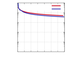
Figure 2(a) shows the relative errors of Algorithm 2 applied to two instances of the class $\operatorname{\bf rand}(16,100,5)$ and to the tensor $\operatorname{\bf cheb}(16,100)$. The convergence rates for $\operatorname{\bf cheb}(16,100)$ as well as for one of the $\operatorname{\bf rand}(16,100,5)$-tensors tend to one as indicated by (25). The other instance of $\operatorname{\bf rand}(16,100,5)$ shows a linear convergence with a convergence rate of $\approx 0.52$.

(a) Relative errors of Algorithm 2 applied to two tensors of type $\operatorname{\bf rand}(16,100,5)$ and to the tensor $\operatorname{\bf cheb}(16,100)$. The convergence can be very slow with a convergence rate tending to one, cf. (25).

(b) Algorithm 4 applied to the tensor $\operatorname{\bf cheb}(16,100)$ together with the corresponding results from Figure 4(b) (Algorithms 2 and 3).

Figure 2: Algorithms 2 and 4 applied to example tensors.

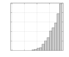
In order to get an impression of how likely the slow convergence behavior (25) occurs for Algorithm 2, we measured the convergence rates of Algorithm 2 for 1000 random tensors of $\operatorname{\bf rand}(16,1000,5)$. The resulting histogram is depicted in Figure 3(a): in $24.6\%$ of the cases a convergence rate larger than $0.95$ was measured; a convergence rate of $0.75$ or better was observed in $19.2\%$ of the cases. These results indicate that the sole power iteration in general converges quite slowly.

(a) Algorithm 2

(b) Algorithm 3 ($k=5$)

Figure 3: Convergence rates of Algorithm 2 and Algorithm 3 (with $k=5$) for 1000 random tensors of the class $\operatorname{\bf rand}(16,1000,5)$. We used the same 1000 tensors for both algorithms.

8.1.1 Measurement of the convergence rate

The convergence rates in Figures 3 and 5 have been taken as the quotient $\mathrm{error}_{j}/\mathrm{error}_{j-1}$, where $j$ is the last step with a relative error larger than $10^{-12}$. For Algorithms 2, 3, 4 we performed 40 steps in total, whereas the number of steps in Algorithm 5 is chosen adaptively, cf. Section 6.

8.2 Power iteration with Rayleigh-Ritz method (Algorithm 3)

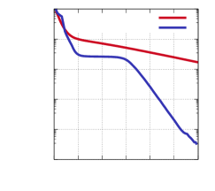
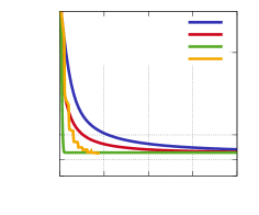
In Figure 4 we apply Algorithm 3 to the slowly converging tensors from Figure 2(a). It turns out that in one case (the slowly converging instance of $\operatorname{\bf rand}(16,100,5)$ from Figure 2(a)) we get linear convergence of Algorithm 3, whereas the convergence rate for $\operatorname{\bf cheb}(16,100)$ still tends to one, i.e. the convergence behavior does not improve in this case.

(a) $\operatorname{\bf rand}(16,100,5)$

(b) $\operatorname{\bf cheb}(16,100)$

Figure 4: Improvement achieved by Algorithm 3 (with $k=5$) applied to the slowly converging tensors from Figure 2(a): for the $\operatorname{\bf rand}(16,100,5)$-tensor Algorithm 3 now shows linear convergence with rate $\approx 0.71$, whereas the convergence behavior for $\operatorname{\bf cheb}(16,100)$ is still bad (convergence rate tending to one).

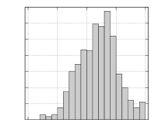
In order to get an idea of how much Algorithm 3 improves Algorithm 2, we applied Algorithm 3 to the same 1000 tensors which have been used for the histogram in Figure 3(a), cf. Figure 3(b). Based on Figure 3, Algorithm 3 seems to yield a notable acceleration of the convergence speed. Notice, however, that Figure 3 only reflects the the class $\operatorname{\bf rand}(16,1000,5)$ of random tensors.

For our experiments we used a Rayleigh-Ritz method w.r.t. the latest $k=5$ iterates in each step, i.e. the subspace (26) has dimension $5$. In order to compare Algorithms 1 and 3, we applied the Rayleigh-Ritz method in each step of Algorithm 3. In all of our experiments $k=5$ has proven to be a suitable choice: the average relative error for 100 instances of $\operatorname{\bf rand}(d,n,4)$ after 100 steps of power iteration and subsequent Rayleigh-Ritz method with subspace dimension $k$ was minimized for $k=5$ or $k=6$, regardless of the tensor size. If $k$ is chosen too small, the resulting Rayleigh-Ritz method has only little effect. If, on the other hand, $k$ is chosen too large, the orthogonalization (HT-QR followed by a truncation, cf. Section 5.1) might not be exact enough which seems to lead to even higher errors than without the Rayleigh-Ritz method.

Compared to the overall computational work of the power iteration, the effort for the subsequent Rayleigh-Ritz method is small.

8.3 Power iteration with squaring (Algorithm 4)

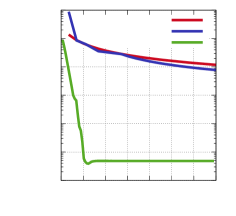
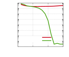
A significant acceleration of the convergence can be achieved by using Algorithm 4 described in Section 6. The resulting relative errors for the tensor $\operatorname{\bf cheb}(16,100)$ are depicted in Figure 2(b) in comparison with the errors from Figure 4(b): Algorithm 4 converges almost instantaneously to a relative error of about $5\cdot 10^{-6}$, where it stagnates due to truncations of the iterates down to lower HT-representation ranks.

Figure 5(a) shows the corresponding histogram for Algorithm 4 applied to the same 1000 tensors used for Figure 3: as predicted in Section 6, cf. (32), in most cases we observe a convergence rate of less than $0.5$. However, in $5.8\%$ of the cases the convergence rate is close to one, which reflects those cases where Algorithm 4 does not converge (i.e. stagnates early) because of the truncation errors becoming to large, cf. (33), (34). This stability issue of Algorithm 4 can be improved by using Algorithm 5 which is an adaptive combination of Algorithms 3 and 4: first a good enough starting vector is computed by the more stable Algorithm 3 and then the fast convergence of Algorithm 4 is exploited using this starting vector, cf. Section 6.

(a) Algorithm 4

(b) Algorithm 5

Figure 5: Convergence rates of Algorithms 4 and 5 for the same 1000 tensors of $\operatorname{\bf rand}(16,1000,5)$ as in Figure 3: we measured very small convergence rates far below $0.25$. In $58/1000$ cases Algorithm 4 does not converge (i.e. stagnates early) because of too large truncation errors, cf. (34). For $44$ (i.e. $75\%$) of these tensors, however, convergence can be achieved by using Algorithm 5 instead. In Algorithm 5 we applied $N_{3}=10$ more steps of Algorithm 3 in each cycle.

8.4 Power iteration with squaring and stabilization (Algorithm 5)

In Figure 6(a) we give an example of a tensor for which Algorithm 4 does not converge, whereas Algorithm 5 (including 2 steps of Algorithm 3 for the computation of the starting tensor) converges. The example tensor of Figure 6(a) was found as random tensor generated by the MATLAB toolbox htucker [17].

(a) An example tensor (order $d=8$ with $12\,288$ entries) for which Algorithm 4 does not converge whereas Algorithm 5 (including only two steps of Algorithm 3) does.

(b) A counterexample $\mathbf{a}\in\mathbb{R}^{I}$ defined by (39), (40), for which none of our algorithms approximates well the maximum norm $\|\mathbf{a}\|_{\infty}$: the relative error of all methods stays above $0.47$.

Figure 6: Counterexamples

In Figure 5(b) we apply Algorithm 5 to the same 1000 tensors as in Figure 5(a) (and in Figure 3): we now get convergence for $75\%$ of the cases where Algorithm 4 did not converge.

8.5 An example where the algorithms fail

Based on (11) we can construct tensors $\mathbf{a}\in\mathbb{R}^{I}$, $I=\bigtimes_{\mu=1}^{d}I_{\mu}$, for which our algorithms fail: the tensor entry $\mathbf{a}[\mathbf{i}]$ which maximizes $|\mathbf{a}[\mathbf{i}]|$ is deleted by truncations which results in the algorithms no longer converging to $\|\mathbf{a}\|_{\infty}$. As an example take a tensor $\mathbf{a}\in\mathbb{R}^{I}$, $I=\bigtimes_{\mu=1}^{d}I_{\mu}$, with $d=10$ and mode sizes $\#I_{\mu}=n$, $\mu=1,\ldots,d$, defined by

$$\mathbf{a}:=\left(\begin{array}[]{r}\mbox{\tt rand}[0.91,1.0]\\ \vdots\\ \mbox{\tt rand}[0.91,1.0]\end{array}\right)\otimes\cdots\otimes\left(\begin{array}[]{r}\mbox{\tt rand}[0.91,1.0]\\ \vdots\\ \mbox{\tt rand}[0.91,1.0]\end{array}\right)$$ (39)

at all indices $\mathbf{i}\neq(1,\ldots,1)$ and

$$\mathbf{a}[1,\ldots,1]:=1.9.$$ (40)

The elementary tensor (39) has HT-rank $(1,\ldots,1)$ and the extra definition (40) increases the components of the HT-rank to $2$. The resulting tensor $\mathbf{a}$ contains entries in $[0.1,1.0]$ at all indices $\mathbf{i}\neq(1,\ldots,1)$ and attains its maximum $1.9$ at $(1,\ldots,1)$, i.e. $\|\mathbf{a}\|_{\infty}=1.9$. As shown in Figure 6(b), none of the methods presented in this article approximates well the maximum norm $\|\mathbf{a}\|_{\infty}$: the relative errors stay above $0.47$ which corresponds to a computed maximum norm of less than $1.007$ instead of $1.9$.

8.6 Finding the maximizing index by a binary search (Algorithm 6)

In Figure 7 the runtimes of Algorithms 5 and 6 are displayed, once for varying tensor order $d$ and once for varying mode sizes $n$. As expected, we find the runtime of Algorithm 5 to depend linearly on the tensor order $d$, whereas the runtime of Algorithm 6 in the end grows quadratically with $d$, cf. (38). Also the dependence of the runtime on $n$ behaves as expected: finally both algorithms seem to grow linearly with $n$.

(a) $\operatorname{\bf cheb}(d,100)$, $d=4,8,\ldots,128$

(b) $\operatorname{\bf cheb}(16,n)$, $n=2,10,100,\ldots,100\,000$

Figure 7: Runtimes of Algorithms 5 and 6 for the tensor $\mathbf{a}=\operatorname{\bf cheb}(d,n)$ with tensor orders $d=4,8,\ldots,128$ and mode sizes $n=10,100,\ldots,1\,000\,000$. For all values of $d$ and $n$ the corresponding relative approximation error of $\|\mathbf{a}\|_{\infty}$ lies between $2\cdot 10^{-10}$ and $5\cdot 10^{-4}$.

9 Conclusions

In this article we have shown how extreme entries in low-rank tensors can be approximated using a power iteration. The resulting algorithms can be applied for any low-rank tensor format which meets the requirements stated at the end of Section 2. We presented two approaches how to accelerate the generally slowly converging power iteration. The algorithm which we suggest is an adaptive combination of these accelerated methods. A binary search makes it possible to also find an according extreme entry of the tensor, i.e. find a tensor index which maximizes the absolute value of tensor entries. Our experiments in Section 8 indicate that our algorithms work well for many tensors, cf. Figures 5 and 7. Even for those tensors of Figure 5 for which the convergence of Algorithms 4 or 5 stagnates early, the maximum relative error is $4\cdot 10^{-3}$, which would still be of good use in many applications.

The maximum norm estimator of our algorithm approximates the maximum norm from below (i.e. yields a lower bound), cf. Lemma 7. In order to use a branch and bound algorithm it would be interesting to have useful upper bounds for the maximum norm.

References

- [1] Z. Bai, J. Demmel, J. Dongarra, A. Ruhe, and H. van der Vorst, Templates for the Solution of Algebraic Eigenvalue Problems, Society for Industrial and Applied Mathematics, 2000.
- [2] Richard E. Bellman, Adaptive Control Processes: A Guided Tour, MIT Press, 1961.
- [3] Richard Ernest Bellman, Dynamic Programming, Dover Publications, Inc., New York, NY, USA, 2003.
- [4] V. de Silva and L. Lim, Tensor Rank and the Ill-Posedness of the Best Low-Rank Approximation Problem, SIAM Journal on Matrix Analysis and Applications, 30 (2008), pp. 1084–1127.
- [5] Mike Espig, Effiziente Bestapproximation mittels Summen von Elementartensoren in hohen Dimensionen, dissertation, Universität Leipzig, 2007.
- [6] Mike Espig, Wolfgang Hackbusch, Alexander Litvinenko, Hermann G. Matthies, and Elmar Zander, Post-processing of high-dimensional data, arxiv, (2019). https://arxiv.org/abs/1906.05669.
- [7] Gene H. Golub and Charles F. Van Loan, Matrix Computations, Johns Hopkins University Press, Baltimore, MD, USA, 3rd ed., 1996.
- [8] Lars Grasedyck, Hierarchical Singular Value Decomposition of Tensors, SIAM Journal on Matrix Analysis and Applications, 31 (2010), pp. 2029–2054.
- [9] Lars Grasedyck, Polynomial Approximation in Hierarchical Tucker Format by Vector-Tensorization, tech. report, 2010.
- [10] Lars Grasedyck, Daniel Kressner, and Christine Tobler, A literature survey of low-rank tensor approximation techniques, GAMM-Mitteilungen, 36 (2013), pp. 53–78.
- [11] Lars Grasedyck and Christian Löbbert, Distributed hierarchical SVD in the Hierarchical Tucker format, Numerical Linear Algebra with Applications, 25 (2018), p. e2174.
- [12] Wolfgang Hackbusch, Tensor spaces and numerical tensor calculus, vol. 42 of Springer Ser. Comput. Math., Springer, Heidelberg, 2012.
- [13] Wolfgang Hackbusch, Boris N. Khoromskij, and Eugene E. Tyrtyshnikov, Approximate iterations for structured matrices, Numerische Mathematik, 109 (2008), pp. 365–383.
- [14] Frank L. Hitchcock, The Expression of a Tensor or a Polyadic as a Sum of Products, Journal of Mathematics and Physics, 6 (1927), pp. 164–189.
- [15] Johan Håstad, Tensor rank is NP-complete, Journal of Algorithms, 11 (1990), pp. 644 – 654.
- [16] Donald E. Knuth, The Art of Computer Programming, Sorting and Searching, vol. 3, Addison Wesley Longman Publishing Co., Inc., Redwood City, CA, USA, 2nd ed., 1998.
- [17] Daniel Kressner and Christine Tobler, Algorithm 941: Htucker – A MATLAB Toolbox for Tensors in Hierarchical Tucker Format, ACM Trans. Math. Softw., 40 (2014), pp. 22:1–22:22.
- [18] J. Kuczyński and H. Woźniakowski, Estimating the Largest Eigenvalue by the Power and Lanczos Algorithms with a Random Start, SIAM Journal on Matrix Analysis and Applications, 13 (1992), pp. 1094–1122.
- [19] Christian Löbbert, Parallel algorithms for tensor arithmetic in low-rank formats and applications, dissertation, RWTH Aachen, 2019.
- [20] Ivan Oseledets, Tensor-Train Decomposition, SIAM Journal on Scientific Computing, 33 (2011), pp. 2295–2317.
- [21] F. Verstraete and J. I. Cirac, Matrix product states represent ground states faithfully, Phys. Rev. B, 73 (2006).
- [22] Guifré Vidal, Efficient classical simulation of slightly entangled quantum computations, Physical review letters, 91 (2003).