Quantum-Inspired Hamiltonian Monte Carlo for Bayesian Sampling

Abstract

Hamiltonian Monte Carlo (HMC) is an efficient Bayesian sampling method that can make distant proposals in the parameter space by simulating a Hamiltonian dynamical system. Despite its popularity in machine learning and data science, HMC is inefficient to sample from spiky and multimodal distributions. Motivated by the energy-time uncertainty relation from quantum mechanics, we propose a Quantum-Inspired Hamiltonian Monte Carlo algorithm (QHMC). This algorithm allows a particle to have a random mass matrix with a probability distribution rather than a fixed mass. We prove the convergence property of QHMC and further show why such a random mass can improve the performance when we sample a broad class of distributions. In order to handle the big training data sets in large-scale machine learning, we develop a stochastic gradient version of QHMC using Nosé-Hoover thermostat called QSGNHT, and we also provide theoretical justifications about its steady-state distributions. Finally in the experiments, we demonstrate the effectiveness of QHMC and QSGNHT on synthetic examples, bridge regression, image denoising and neural network pruning. The proposed QHMC and QSGNHT can indeed achieve much more stable and accurate sampling results on the test cases.

Keywords: Hamiltonian Monte Carlo, Quantum-Inspired Methods, Sparse Modeling

1 Introduction

Hamiltonian Monte Carlo (HMC) (Duane et al., 1987; Neal et al., 2011) improves the traditional Markov Chain Monte Carlo (MCMC) method  (Hastings, 1970) by introducing an extra momentum vector $\mathbf{q}$ conjugate to a state vector $\mathbf{x}$. In MCMC, a particle is usually only allowed to randomly walk in the state space. However, in HMC, a particle can flow quickly along the velocity direction and make distant proposals in the state space based on Hamiltonian dynamics. The energy-conservation property in continuous Hamiltonian dynamics can largely increase the acceptance rate, resulting in much faster mixing rate than standard MCMC. In numerical simulations where continuous time is quantized by discrete steps, the Metropolis-Hastings (MH) correction step can guarantee the correctness of the invariant distribution. HMC plays an increasingly important role in machine learning (Springenberg et al., 2016; Myshkov and Julier, 2016).

HMC requires computation of the gradients of the energy function, which is the negative logarithm of the posterior probability in a Bayesian model. Therefore, HMC is born for smooth and differentiable functions but not immediate for non-smooth functions. In the case where functions have discontinuities, extra reflection and refraction steps (Mohasel Afshar and Domke, 2015; Nishimura et al., 2017) need to be involved in order to enhance the sampling efficiency. In the case characterized by $\ell_{p}$ prior where $1\leq p<2$, proximity operator methods (Chaari et al., 2016, 2017) can be used to increase the accuracy for simulating the Hamiltonian dynamics.

This paper aims to develop a new type of HMC method in order to sample efficiently from a possibly spiky or multimodal posterior distribution. A representative example is Bayesian model of sparse or low-rank modeling using an $\ell_{p}$ ($0<p\leq 1$) norm as the penalty. It is shown that sparser models can be obtained because $\ell_{p}$ $(0<p<1)$ prior (Zhao et al., 2014; Xu et al., 2010) is a better, although non-convex, approximation for $\ell_{0}$ norm (Polson and Sun, 2019) than $\ell_{1}$ norm that is widely used in compressed sensing (Donoho et al., 2006; Eldar and Kutyniok, 2012) and model reductions (Hou et al., 2018).

Leveraging the energy-time uncertainty relation in quantum mechanics, this paper proposes a quantum-inspired HMC (QHMC) method. In quantum mechanics, a particle can have a mass distribution other than a fixed mass value. Although being a pedagogical argument from physics, we will show from both theories and experiments that this principle can actually help achieve better sampling efficiency for non-smooth functions than standard HMC with fixed mass. The main idea of QHMC is visualized in Fig. 1 with a one-dimensional harmonic oscillator. Assume that we have a ball with mass $m$ attached to a spring at the origin. The restoring force exerted on the ball pulls the ball back to the origin and the magnitude of the force is proportional to the displacement $x$, i.e., $F=-kx$. The ball oscillates around the origin with the time period $T=2\pi\sqrt{\frac{m}{k}}$. In standard HMC, $m$ is fixed and usually set as 1. In contrast, QHMC allows $m$ to be time-varying, meaning that the particle is sometimes moving fast and sometimes moving slowly. This is equivalent to employing a varying time scale. Consequently, different distribution landscapes can be explored more effectively with different time scales. In a flat but broad region, QHMC can quickly scan the whole region with a small time period $T$ (or small $m$). In a spiky region, we need to carefully explore every corner of the landscape, therefore a large $T$ (or large $m$) is preferred. In standard HMC, it is hard to choose a fixed time scale or mass to work well for both cases. This physical intuition is similar to the key idea of randomized HMC (Bou-Rabee and Sanz-Serna, 2017), but this work consider more general cases where the mass can be a positive definite matrix $\mathbf{M}$.

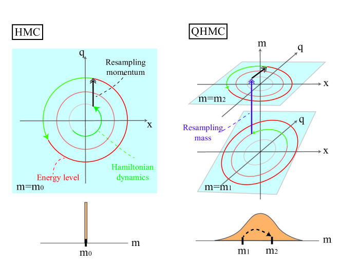
Figure 1: Illustration of Quantum-Inspired Hamiltonian Monte Carlo (QHMC) with the simple case of a one-dimensional harmonic oscillator. For HMC, the trajectories (energy levels) are confined in $(x,q)$ space with fixed mass. For QHMC, the mass is the third dimension that needs sampling. Here we use a scalar mass for illustration, however in general our framework allows the mass to be a positive definite matrix.

This paper is organized as follows. In Section 2, we review the standard HMC and summarize several HMC variants that are related to the physics literature. In Section 3, we propose the novel QHMC algorithm that treats mass as a random (positive definite) matrix rather than a fixed real positive scalar. We investigate the convergence properties of QHMC and demonstrate the advantages of QHMC with some toy examples on which HMC fails to work. Section 4 explains why treating the mass as a random variable improves the sampling performance for a large class of distributions. Section 5 proposes quantum stochastic gradient Nosé-Hoover thermostat (QSGNHT) to implement QHMC with massive training data, and proves its convergence based on stochastic differential equations (SDE). In Section 6, we use both synthetic and realistic examples to demonstrate the effectiveness of QHMC and QSGNHT. They can avoid parameter tunings and achieve superior accuracy for a wide range of distributions, especially for spiky and multi-modal ones that are common in Bayesian learning.

Input: starting point $\mathbf{x_{0}}$, step size $\epsilon$, simulation steps $L$, mass $\mathbf{M}=m\mathbf{I}$.

for $t=1,2,\cdots$ do

       Resample $\mathbf{q}\sim{\cal N}(0,\mathbf{M})$;

       ($\mathbf{x}_{0},\mathbf{q}_{0}$)=($\mathbf{x}^{(t)},\mathbf{q}^{(t)}$);

       Simulate dynamics based on Eq. (1);

       $\mathbf{q}_{0}\leftarrow\mathbf{q}_{0}-\frac{\epsilon}{2}\nabla U(\mathbf{x}_{0})$;

       for $i=1,\cdots,L-1$ do

             $\mathbf{x}_{i}\leftarrow\mathbf{x}_{i-1}+\epsilon\mathbf{M}^{-1}\mathbf{q}_{i-1}$;

             $\mathbf{q}_{i}\leftarrow\mathbf{q}_{i-1}-\epsilon\nabla U(\mathbf{x}_{i})$

       end for

      $\mathbf{x}_{L}\leftarrow\mathbf{x}_{L-1}+\epsilon\mathbf{M}^{-1}\mathbf{q}_{L-1}$;

       $\mathbf{q}_{L}\leftarrow\mathbf{q}_{L-1}-\frac{\epsilon}{2}\nabla U(\mathbf{x}_{L})$;

       ($\hat{\mathbf{x}},\hat{\mathbf{q}}$)=($\mathbf{x}_{L},\mathbf{q}_{L}$);

       M-H step: $u\sim\mathrm{Uniform[0,1]}$;

       $\rho=e^{-H(\hat{\mathbf{x}},\hat{\mathbf{q}})+H(\mathbf{x}^{(t)},\mathbf{q}^{(t)})}$;

       if $u<\mathrm{min}(1,\rho)$ then

            $(\mathbf{x}^{(t+1)},\mathbf{q}^{(t+1)})=(\hat{\mathbf{x}},\hat{\mathbf{q}})$

      else

            $(\mathbf{x}^{(t+1)},\mathbf{q}^{(t+1)})=(\mathbf{x}^{(t)},\mathbf{q}^{(t)})$

       end if

      

end for

Output: $\{\mathbf{x}^{(1)},\mathbf{x}^{(2)},\cdots\}$

Algorithm 1 Hamiltonian Monte Carlo

2 Hamiltonian Monte Carlo

In Bayesian inference, we want to sample the parameters $\mathbf{x}$ from the posterior distribution $p(\mathbf{x}|{\cal D})$ given the dataset ${\cal D}$. Instead of directly sampling $\mathbf{x}$, HMC introduces an extra momentum variable $\mathbf{q}$, and samples in the joint space of $(\mathbf{x},\mathbf{q})$. By defining a potential function $U(\mathbf{x})=-\mathrm{log}\ p(\mathbf{x}|{\cal D})$ and a kinetic energy $K(\mathbf{q})=\frac{1}{2}\mathbf{q}^{T}\mathbf{M}_{0}^{-1}\mathbf{q}$ where $\mathbf{M}_{0}$ is a time-independent positive-definite mass matrix, HMC (Duane et al., 1987; Neal et al., 2011) samples from the joint density of $(\mathbf{x},\mathbf{q})$ by simulating the following Hamiltonian dynamics:

$$d\begin{pmatrix}\mathbf{x}\\ \mathbf{q}\end{pmatrix}=dt\begin{pmatrix}\mathbf{M}_{0}^{-1}\mathbf{q}\\ -\nabla U(\mathbf{x})\end{pmatrix}$$ (1)

The resulting steady-state distribution is

$$\pi(\mathbf{x},\mathbf{q})\propto{\rm exp}\left(-\beta U\left(\mathbf{x}\right)-\beta K\left(\mathbf{q}\right)\right).$$ (2)

where $\beta=1/k_{B}T$  and is set as 1 in standard HMC. Because $\mathbf{x}$ and $\mathbf{q}$ are independent with each other, one can easily marginalize the joint density over $\mathbf{q}$ to obtain the invariant distribution in the parameter space $\pi(\mathbf{x})\propto{\rm exp}(-U(\mathbf{x}))=p(\mathbf{x}|{\cal D})$.

The algorithm flow of a standard HMC is summarized in Alg. 1. The HMC sampler switches between two steps: 1) travel on a constant energy surface according to Hamiltonian dynamics in Eq. (1) with step size $\epsilon$ and number of simulation steps $L$, and 2) maintain state $\mathbf{x}$ but resample momentum $\mathbf{q}$ to transit to another energy surface. In order to guarantee volume preservation and accuracy of the simulations (Neal et al., 2011), the “leapfrog" integrator is commonly used in HMC. In practice, one needs to choose a step size $\epsilon$ to discretize the continuous time $t$, and the number of simulation steps $L$ to decide how many steps the dynamics runs before resampling the momentum.

However, the performance of a standard HMC can degrade due to the following limitations:

• Ill-conditioned distribution: the isotropic mass in HMC assumes the target distribution has the same scale in all directions, so HMC is poor at exploring ill-conditioned distributions, e.g., a Gaussian distribution with a covariance matrix whose eigenvalues have a wide spread.

• Multimodal distribution: although the momentum variable can help the particle reach higher energy levels than MCMC, it is still hard for HMC to explore multimodal distributions because of the fixed temperature ($k_{B}T=1$).

• Stochastic implementation: standard HMC involves full gradient computations over the whole data set. This can be very expensive when dealing with big-data problems.

• Non-smooth distribution: HMC needs computing gradients of the energy function, therefore it can behave badly or even fail for non-smooth (discontinuous or spiky) functions.

It is interesting to note that some physical principles have been employed to overcome some aforementioned limitations of HMC. Specifically, magnetic HMC (Tripuraneni et al., 2017) can efficiently explore multimodal distributions by introducing magnetic fields; Stochastic gradient HMC improves the efficiency of handling large data set by simulating the second-order Langevin dynamics (Chen et al., 2014); The relativistic HMC (Lu et al., 2016) achieves a better convergence rate due to the analogy between the speed of light and gradient clipping; The reflection and refraction HMC (Mohasel Afshar and Domke, 2015) leverages optics theory to efficiently sample from discontinuous distributions; The wormhole HMC (Lan et al., 2014), motivated by Einstein’s general relativity, builds shortcuts between two modes; Also inspired by general relativity, the Riemannian HMC (Girolami and Calderhead, 2011) can adapt a mass matrix pre-conditioner according to the geometry of a Riemannian manifold, which can better handle ill-conditioned distributions; Randomized HMC (Bou-Rabee and Sanz-Serna, 2017), a special case of our work, models the lifetime of a path as an exponential distribution which is a common assumption in thermodynamics. Table 1 has summarized some representative HMC algorithms and their corresponding physical models.

Inspired by quantum mechanics, this work constructs a stochastic process with a time-varying mass matrix, aiming to sample efficiently from a possibly spiky or multi-modal distribution. Our method can be combined with other methods due to its efficiency (nearly no extra cost) and flexibility.

Table 1: Summary of various HMC methods.

Challenges to address	HMC variants	Physic theory
Ill-conditioned distribution	RMHMC (Girolami and Calderhead, 2011)	General relativity
Multimodal dist.	Magnetic HMC (Tripuraneni et al., 2017)	Electromagnetism
	Wormhole HMC (Lan et al., 2014)	General relativity
	Tempered HMC (Graham and Storkey, 2017)	Thermodynamics
	RHMC (Bou-Rabee and Sanz-Serna, 2017)	Thermodynamics
	Fractional HMC (Ye and Zhu, 2018)	Lévy Process
Large training data set	Stochastic Gradient HMC (Chen et al., 2014)	Langevin dynamics
	Thermostat HMC (Ding et al., 2014)	Thermodynamics
	Relativistic HMC (Lu et al., 2016)	Special relativity
Discontinuous dist.	Optics HMC (Mohasel Afshar and Domke, 2015)	Optics
Spiky & multimodal dist.	Quantum-inspired HMC (this work)	Quantum mechanics

3 Quantum-Inspired Hamiltonian Monte Carlo

In this section, we propose the physical model and numerical implementation of a quantum-inspired Hamiltonian Monte Carlo (QHMC). In Section 3.2 and 3.3 we prove that its resulting steady-state distribution and time-averaged distribution are indeed the targeted posterior distribution $p(\mathbf{x}|{\cal D})$. In Section 3.4, we discuss a few possible extensions of QHMC.

3.1 QHMC Model and Algorithm

Different from HMC that simulates the Hamiltonian dynamics of a constant mass $\mathbf{M}_{0}$, our QHMC allows $\mathbf{M}(t)$ to be time-varying and random. Specifically, we construct a stochastic process and let each realization be $\mathbf{M}(t)$. In general at each time $t$, $\mathbf{M}(t)$ is sampled independently from a (time-independent) distribution $P_{\mathbf{M}}(\mathbf{M})$. In other words, $\{\mathbf{M}(t_{1}),\mathbf{M}(t_{2}),\cdots,\mathbf{M}(t_{n})\}$ are i.i.d. positive definite matrices. Section 4 will provide some heuristics on how to choose $P_{\mathbf{M}}(\mathbf{M})$ properly. After obtaining a realization of time-varying mass $\mathbf{M}(t)$, we simulate the following dynamical system:

$$d\begin{pmatrix}\mathbf{x}\\ \mathbf{q}\end{pmatrix}=dt\begin{pmatrix}\mathbf{M}(t)^{-1}\mathbf{q}\\ -\nabla U(\mathbf{x})\end{pmatrix}$$ (3)

where we assume that $U(\mathbf{x})$ a differentiable potential energy function with a well-defined gradient $\nabla U(\mathbf{x})$ everywhere, except for some points with zero measure . The discretized version of Eq. (3) is

$$\left\{\begin{aligned} &\mathbf{q}_{i+\frac{1}{2}}\leftarrow\ \mathbf{q}_{i}-\frac{\epsilon}{2}\nabla U(\mathbf{x}_{i}).\\ &\mathbf{x}_{i+1}\leftarrow\ \mathbf{x}_{i}+\epsilon\mathbf{M}_{t}^{-1}\mathbf{q}_{i+\frac{1}{2}}\quad\\ &\mathbf{q}_{i+1}\leftarrow\ \mathbf{q}_{i+\frac{1}{2}}-\frac{\epsilon}{2}\nabla U(\mathbf{x}_{i+1}).\\ \end{aligned}\right.$$ (4)

Where $t$ denotes the index of paths, $\mathbf{M}_{t}$ is the mass matrix used for the $t$-th path and is sampled from $P_{\mathbf{M}}(\mathbf{M})$ at the beginning of the path; $i=1,2,\cdots,L$ denotes the index of steps in each path. The resulting numerical algorithm flow is shown in Alg. 2 . The implementation of QHMC is rather simple: compared with HMC, we only need an extra step of resampling the mass matrix. Note that HMC can be regarded as a special case of QHMC: QHMC becomes a standard HMC when $P_{\mathbf{M}}(\mathbf{M})$ is the Dirac delta function $\delta(\mathbf{M}-\mathbf{M}_{0})$.

Physical Intuition: In standard HMC (Duane et al., 1987; Neal et al., 2011) described by Eq. (1), the mass matrix $\mathbf{M}$ is usually chosen as diagonal such that $\mathbf{M}=m\mathbf{I}$ and further the scalar mass $m$ is commonly set as 1. Such a choice corresponds to the classical physics where the mass is scalar and deterministic. In the quantum physics, however, the energy and time obeys the following uncertainty relationship:

$$\Delta E\Delta t\approx\hbar.$$ (5)

Here $\Delta E$ is the uncertainty of the static energy for a particle, and $\Delta t$ is seen as length of time the particle can survive (lifetime), and $\hbar\sim 1.05\times 10^{-34}$ is the Planck constant. Moreover, based on the well-known mass-energy relation discovered by Albert Einstein

$$E=mc^{2},$$ (6)

we know that the mass of a particle is proportional to its static energy. Combining Eq. (5) and (6), we conclude $\Delta m\approx\hbar/(c^{2}\Delta t)$, indicating that a quantum particle can have a random mass obeying the distribution $P_{m}(m)$ (more generally $P_{\mathbf{M}}(\mathbf{M})$), or equivalently, each realization of the stochastic process can produce a time-varying mass $\mathbf{M}=\mathbf{M}(t)$ . In quantum mechanics, the mass distribution $P_{\mathbf{M}}(\mathbf{M})$ is only dependent on the types of the quantum particles, therefore we assume that $P_{\mathbf{M}}(\mathbf{M})$ is independent of $\mathbf{x}$ and $\mathbf{q}$ in this manuscript. Without this assumption, a wrong distribution may be produced, which will be shown in Section 3.3.

To avoid possible confusions, we would like to state explicitly that the dynamics described by Eq. (3) is not a completely quantum model because both $\mathbf{x}$ and $\mathbf{q}$ are deterministic once an initial condition and a specific realization of $\mathbf{M}(t)$ are given. Indeed a classical computer will probably not solve a quantum system with a lower computational cost than its classical counterpart.

Input: starting point $\mathbf{x}_{0}$, step size $\epsilon$, simulation steps $L$, and mass distribution $P_{\mathbf{M}}(\mathbf{M})$

(For D-QHMC and S-QHMC, $P_{\mathbf{M}}(\mathbf{M})$ requires parameters $\vec{\mu}_{m}$/ $\vec{\sigma}_{m}$ and $\mu_{m}$/$\sigma_{m}$).

for $t=1,2,\cdots$ do

       Resample $\mathbf{M}_{t}\sim P_{\mathbf{M}}(\mathbf{M})$;

        [D-QHMC: $\omega_{k}\sim\mathcal{N}(\mu_{m}^{(k)},\sigma_{m}^{(k)2}),m_{kk}=10^{\omega_{k}},\mathbf{M}=\text{diag}(m_{11},\cdots,m_{dd})$];

        [S-QHMC: $\omega\sim\mathcal{N}(\mu_{m},\sigma_{m}^{2}),m_{kk}=10^{\omega},\mathbf{M}=m\mathbf{I}$];

      

      Resample $q\sim{\cal N}(0,\mathbf{M})$;

       ($\mathbf{x}_{0},\mathbf{q}_{0}$)=($\mathbf{x}^{(t)},\mathbf{q}^{(t)}$);

       Simulate dynamics based on Eq. (2);

       $\mathbf{q}_{0}\leftarrow\mathbf{q}_{0}-\frac{\epsilon}{2}\nabla U(\mathbf{x}_{0})$;

       for $i=1,\cdots,L-1$ do

             $\mathbf{x}_{i}\leftarrow\mathbf{x}_{i-1}+\epsilon\mathbf{M}_{t}^{-1}\mathbf{q}_{i-1}$;

             $\mathbf{q}_{i}\leftarrow\mathbf{q}_{i-1}-\epsilon\nabla U(\mathbf{x}_{i})$

       end for

      $\mathbf{x}_{L}\leftarrow\mathbf{x}_{L-1}+\epsilon\mathbf{M}_{t}^{-1}\mathbf{q}_{L-1}$;

       $\mathbf{q}_{L}\leftarrow\mathbf{q}_{L-1}-\frac{\epsilon}{2}\nabla U(\mathbf{x}_{L})$;

       ($\hat{\mathbf{x}},\hat{\mathbf{q}}$)=($\mathbf{x}_{L},\mathbf{q}_{L}$);

       M-H step: $u\sim\mathrm{Uniform[0,1]}$;

       $\rho=e^{-H(\hat{\mathbf{x}},\hat{\mathbf{q}})+H(\mathbf{x}^{(t)},\mathbf{q}^{(t)})}$;

       if $u<\mathrm{min}(1,\rho)$ then

            $(\mathbf{x}^{(t+1)},\mathbf{q}^{(t+1)})=(\hat{\mathbf{x}},\hat{\mathbf{q}})$

      else

            $(\mathbf{x}^{(t+1)},\mathbf{q}^{(t+1)})=(\mathbf{x}^{(t)},\mathbf{q}^{(t)})$

       end if

      

end for

Output: $\{\mathbf{x}^{(1)},\mathbf{x}^{(2)},\cdots\}$

Algorithm 2 Quantum-inspired Hamiltonian Monte Carlo (QHMC)

3.2 Steady-State Distribution of QHMC (Space Domain)

Now we show that the continuous-time stochastic process in Eq. (3) and the discrete version in Eq. (4) and Alg. 2 can produce a correct steady distribution that describes the desired posterior density $p(\mathbf{x}|{\cal D})\sim{\rm exp}(-U(\mathbf{x}))$.

Theorem 1

Consider a continuous-time Hamiltonian dynamics with a deterministic time-varying positive-definite matrix $\mathbf{M}(t)$ in Eq. (3). The time-dependent distribution $p(\mathbf{x},\mathbf{q},t)\propto{\rm exp}(-U(\mathbf{x})-\frac{1}{2}\mathbf{q}^{T}\mathbf{M}(t)^{-1}\mathbf{q})$ satisfies the Fokker-Planck equation of Eq. (3). Furthermore, the marginal density $p_{s}(\mathbf{x})\propto{\rm exp}(-U(\mathbf{x}))$ is a unique steady-state distribution in the $\mathbf{x}$ space if momentum resampling steps $p(\mathbf{q})\propto{\rm exp}(-\frac{1}{2}\mathbf{q}^{T}\mathbf{M}(t)^{-1}\mathbf{q})$ are included.

Theorem 1 is the key result of this work, and we would like to prove it from two perspectives. In Section 3.2.1, we treat $\mathbf{M}(t)$ as a deterministic time scale control parameter. This view admits a nice physical interpretation of a re-scaled Hamiltonian dynamics. Furthermore, the relation between QHMC and randomzied HMC (Bou-Rabee and Sanz-Serna, 2017) is natural to see in this setting. In Section 3.2.2, we treat $\mathbf{M}{(t)}$ similarly with state variables $\mathbf{x}$ and $\mathbf{q}$. This perspective can facilitate the proof with the Bayes rule.

3.2.1 Proof of Theorem 1 from the Perspective of Time Scaling

In Lemma 2, we first prove that any time-modifier $\mathbf{A}(t)$ (the meaning of which will be clear later) in Eq. (7) preserves the correct steady distribution.

Lemma 2

Consider a time-dependent continuous Markov process

$$d\begin{pmatrix}\mathbf{x}\\ \mathbf{q}\end{pmatrix}=dt\begin{pmatrix}\mathbf{A}(t)&0\\ 0&\mathbf{A}(t)\end{pmatrix}\begin{pmatrix}\mathbf{q}\\ -\nabla U(\mathbf{x})\end{pmatrix}$$ (7)

where $\mathbf{A}(t)$ is a deterministic time-varying symmetric matrix. For general symmetric $\mathbf{A}(t)$, we have a steady distribution for Eq. (7) as $p_{s}(\mathbf{x},\mathbf{q})\propto{\rm exp}(-U(\mathbf{x})-\mathbf{q}^{T}\mathbf{q}/2)$. Further if a jump process exists, i.e. the momentum is resampled every time interval $t_{0}$ as $p(\mathbf{q})\propto{\rm exp}(-\mathbf{q}^{T}\mathbf{q}/2)$, then the steady distribution is unique.

Proof  The evolution of probability density $p(\mathbf{x},\mathbf{q})$ for the particles $(\mathbf{x},\mathbf{q})$ in Eq. (7) can be described by the following Fokker-Planck equation :

$$\partial_{t}p+\frac{d\mathbf{x}}{dt}\cdot\nabla_{\mathbf{x}}p+\frac{d\mathbf{q}}{dt}\cdot\nabla_{\mathbf{q}}p=0.$$ (8)

We consider the specific density function $p_{s}(\mathbf{x},\mathbf{q})\propto{\rm exp}(-U(\mathbf{x})-\mathbf{q}^{T}\mathbf{q}/2)$. By setting $d\mathbf{x}/dt=\mathbf{A}(t)\mathbf{q}$, $d\mathbf{q}/dt=-\mathbf{A}(t)\nabla U(\mathbf{x})$ according to Eq. (7) and noticing that $\nabla_{\mathbf{x}}p_{s}=-p_{s}\nabla U(\mathbf{x})$ and $\nabla_{\mathbf{q}}p_{s}=-p_{s}\mathbf{q}$, we have

$$\partial_{t}p_{s}=0.$$ (9)

Therefore $p_{s}(\mathbf{x},\mathbf{q})\propto{\rm exp}(-U(\mathbf{x})-\mathbf{q}^{T}\mathbf{q}/2)$ is a stationary distribution of the time-dependent process described by Eq. (7). If the momentum is resampled for a certain time interval, the steady distribution will not change and the Markov process will be guaranteed as ergodic, because the sufficient conditions for ergodicity (Borovkov, 1998) are (1) irreducibility (2) aperiodicity and (3) positive recurrence, the first two of which are guaranteed by the resampling step as diffusion noise. Condition (3) is holds when $U(\mathbf{x})\to\infty$ for $|\mathbf{x}|\to\infty$ which is a reasonable assumption for energy functions. Once the Markov process is ergodic, the steady distribution should be unique (Borovkov, 1998).  

The physical interpretation of $\mathbf{A}(t)$ can be understood by looking at a special case $\mathbf{A}(t)=a(t)\mathbf{I}$. In this case $a(t)$ can be absorbed into $dt$ as $dt^{\prime}=a(t)dt$, and $a(t)$ increases or shrink the time scale (hence the name “time-modifier”). The steady distribution is by definition independent of time, thus $a(t)$ does not change the steady distribution. Note that Eq. (7) becomes a standard time-independent Hamiltonian dynamics with $\mathbf{M}=\mathbf{I}$ when $\mathbf{A}(t)=\mathbf{I}$.

Now we are ready to prove theorem 1. We show that employing a (deterministic) time-varying mass matrix $\mathbf{M}(t)$ is equivalent to employing a (deterministic) time-modifier $\mathbf{A}(t)$.

Proof  We change variables from $(\mathbf{x},\mathbf{q})$ to $(\mathbf{x}^{\prime},\mathbf{q}^{\prime})$ with the transformation:

$$\left\{\begin{array}[]{ll}\mathbf{x}^{\prime}=&\mathbf{x}\\ \mathbf{q}^{\prime}=&\mathbf{M}(t)^{-1/2}\mathbf{q}\end{array}\right.$$ (10)

where $\mathbf{M}^{-1/2}$ is defined as $\mathbf{V}\mathbf{D}^{-1/2}\mathbf{V}^{T}$ with the diagonalization of $\mathbf{M}$ as $\mathbf{M}=\mathbf{V}\mathbf{D}\mathbf{V}^{T}$. After changing variables, Eq. (3) is transformed to

$$d\begin{pmatrix}\mathbf{x}^{\prime}\\ \mathbf{q}^{\prime}\end{pmatrix}=dt\begin{pmatrix}\mathbf{M}(t)^{-1/2}&0\\ 0&\mathbf{M}(t)^{-1/2}\end{pmatrix}\begin{pmatrix}\mathbf{q}^{\prime}\\ -\nabla U(\mathbf{x}^{\prime})\end{pmatrix}$$ (11)

Because $\mathbf{M}(t)^{-1/2}$ is a symmetric matrix, according to Lemma 2, we have a unique steady distribution for $(\mathbf{x}^{\prime},\mathbf{q}^{\prime})$ such that $p_{s}^{\prime}(\mathbf{x}^{\prime},\mathbf{q}^{\prime})\propto{\rm exp}(-U(\mathbf{x}^{\prime})+\mathbf{q}^{\prime T}\mathbf{q}^{\prime}/2)$. After transforming $(\mathbf{x}^{\prime},\mathbf{q}^{\prime})$ back to the $(\mathbf{x},\mathbf{q})$ space, the distribution $p_{s}(\mathbf{x},\mathbf{q},t)\propto({\rm det}\mathbf{M}(t))^{-\frac{1}{2}}{\rm exp}(-U(\mathbf{x})+\mathbf{q}^{T}\mathbf{M}(t)^{-1}\mathbf{q}/2)$ is dependent on $t$, where ${\rm det}(\mathbf{M}(t))$ arises from the Jacobian of variable transformation:

$$p_{s}(\mathbf{x},\mathbf{q},t)d\mathbf{x}d\mathbf{q} =p^{\prime}_{s}(\mathbf{x}^{\prime},\mathbf{q}^{\prime},t)d\mathbf{x}^{\prime}d\mathbf{q}^{\prime}$$ (12)

$$p_{s}(\mathbf{x},\mathbf{q},t)=p_{s}^{\prime}(\mathbf{x}^{\prime},\mathbf{q}^{\prime},t){\rm det}\begin{pmatrix}\frac{\partial\mathbf{x}^{\prime}}{\partial\mathbf{x}}&\frac{\partial\mathbf{x}^{\prime}}{\partial\mathbf{q}}\\ \frac{\partial\mathbf{q}^{\prime}}{\partial\mathbf{x}}&\frac{\partial\mathbf{q}^{\prime}}{\partial\mathbf{q}^{\prime}}\end{pmatrix} \propto({\rm det}\mathbf{M}(t))^{-\frac{1}{2}}{\rm exp}(-U(\mathbf{x})+\mathbf{q}^{T}\mathbf{M}(t)^{-1}\mathbf{q}/2).$$

After marginalization over the momentum $\mathbf{q}$ we obtain the marginal probability density $p_{s}(\mathbf{x})\propto{\rm exp}(-U(\mathbf{x}))$ , which is again independent of $t$ hence a steady distribution.  

The intuition of Theorem 1 is as follows. The time-varying matrix $\mathbf{M}(t)$ has an effect of increasing or shrinking the time scale, but it does not change the steady distribution in the $\mathbf{x}$ space. As a corollary of Theorem 1, we further show that the steady distribution of our discretized QHMC algorithm indeed is the desired posterior distribution.

Corollary 3

Consider a piecewise $\mathbf{M}(t)$. The continuous time is divided into pieces as $\cdots<t_{n-1}<t_{n}<t_{n+1}<\cdots$ and on each time interval, $\mathbf{M}$ is a constant matrix i.e. $\mathbf{M}(t)=\mathbf{M}_{n}$ if $t_{n}\leq t<t_{n+1}$. By sampling $\mathbf{M}_{n}\sim P_{\mathbf{M}}(\mathbf{M})$ as done in Alg. 2, we have the correct teady distribution $p_{s}(\mathbf{x})\propto{\rm exp}(-U(\mathbf{x}))$ for each interval.

If we assume $\mathbf{M}(t)=m(t)\mathbf{I}$ and interpret $\mathbf{A}(t)=\epsilon(t)\mathbf{I}$ as the continuous matrix version of step size $\epsilon$, then changing the mass is equivalent to changing the step size. From the proof of Theorem 1 we know $\mathbf{M}(t)\sim\mathbf{A}(t)^{-2}$ or $m\sim\epsilon^{-2}$. The equivalence $m\sim\epsilon^{-2}$ can be intuitively understood as the result of a “scaling property" of Eq. (1): given a trajectory $(\mathbf{x}(t),\mathbf{q}(t))$ for a particle with mass $m$, the rescaled trajectory $t\to\alpha t$, $\mathbf{q}\to\alpha\mathbf{q},\mathbf{x}\to\mathbf{x}$ for a particle with mass $m\to\alpha^{2}m$ is just the original trajectory but with a different time scale which also obeys the Hamiltonian dynamics Eq. (1).

Although QHMC with a scalar mass is equivalent to HMC with a randomized step (Bou-Rabee and Sanz-Serna, 2017; Neal et al., 2011), QHMC is a more general formulation because $\mathbf{M}$ can be any positive definite matrix other than proportional to identity. We elaborate the benefits of QHMC over randomized HMC in Section 3.4 and in our numerical experiments.

3.2.2 Proof of Theorem 1 via the Bayes Rule

Alternatively, we can treat $\mathbf{M}$ as additional random variables just like $\mathbf{x}$ and $\mathbf{q}$. Then we can consider the joint distribution $(\mathbf{x},\mathbf{q},\mathbf{M})$ and use the Bayes rule to prove Theorem 1.

Proof  We consider the joint steady distribution $p_{s}(\mathbf{x},\mathbf{q},\mathbf{M})$. Here we have dropped the explicit dependence of $\mathbf{M}$ on $t$ because $\mathbf{M}(t)$ obeys the mass distribution $P_{\mathbf{M}}(\mathbf{M})$ for all $t$. Leveraging Bayesian theorem, we have

$$p_{s}(\mathbf{x},\mathbf{q},\mathbf{M})=p_{s}(\mathbf{x},\mathbf{q}|\mathbf{M})P_{\mathbf{M}}(\mathbf{M})$$ (13)

Recall that $p_{s}(\mathbf{x},\mathbf{q}|\mathbf{M})\propto{\rm exp}(-U(\mathbf{x})){\rm exp(-\frac{1}{2}\mathbf{p}^{T}\mathbf{M}^{-1}\mathbf{p}})$, it immediately implies

$$p_{s}(\mathbf{x})=\int_{\mathbf{q}}\int_{\mathbf{M}}d\mathbf{q}\ d\mathbf{M}\ p_{s}(\mathbf{x},\mathbf{q},\mathbf{M})\propto{\rm exp}(-U(\mathbf{x}))$$ (14)

which means the marginal steady distribution $p_{s}(\mathbf{x})$ is the correct posterior distribution.  

The proof relies on two facts: (1) $\mathbf{M}$ itself has a steady distribution in time (i.i.d. for QHMC); (2) $\mathbf{M}$ should not depend explicitly on $\mathbf{x}$, otherwise the samples from the simulated dynamics will produce the wrong posterior distribution, as we will show below.

3.3 Time-Averaged Distribution (Time Domain)

We still need to show that the time-averaged distribution of QHMC is our desired result. The reason is as follows: rather than simulating a set of particles simultaneously, HMC-type methods simulate one particle after another, and collect a set of samples at a sequence of time points. Therefore, the time-averaged distribution $p_{t}(\mathbf{x})$, rather than the space-averaged distribution (steady distribution $p_{s}(\mathbf{x})$), is our final obtained sample distribution. Here the time-averaged distribution is defined as:

$$p_{t}(\mathbf{x})=\left\{\begin{array}[]{lc}\underset{T\to\infty}{{\rm lim}}\frac{1}{T}\sum_{t=0}^{T}\mathbbm{1}(\mathbf{x}(t)=\mathbf{x})&({\rm discrete})\\ \underset{T\to\infty}{{\rm lim}}\frac{1}{T}\int_{0}^{T}\delta(\mathbf{x}(t)-\mathbf{x})dt&({\rm continuous})\\ \end{array}\right.$$ (15)

Where $\mathbbm{1}(\mathbf{x}=\mathbf{x})$ is the indicator function (1 if the argument in the bracket is true and 0 otherwise), and $\delta(\mathbf{x}(t)-\mathbf{x})$ is the Dirac delta function ($+\infty$ if the number in the bracket is 0 and 0 otherwise, plus a normalization criteria as $\int_{\mathbf{x}}\delta(\mathbf{x}(t)-\mathbf{x})d\mathbf{x}=1$) . The physical meaning of $p_{t}(\mathbf{x})$ corresponds to drawing a histogram of samples obtained in the time sequence in HMC and $T$ is the number of simulation paths. In most HMC methods where the step size or mass is fixed, the equivalence between $p_{s}(\mathbf{x})$ and $p_{t}(\mathbf{x})$ can be justified with ergodicity theory from the mathematical perspective (Gray and Gray, 1988; Rosenthal, 1995; Bakry et al., 2008) or ensemble theory from the physical perspective (Eckart, 1953; Oliveira and Werlang, 2007). Also Eq. (1) has the steady distribution $p_{s}(\mathbf{x})=p(\mathbf{x}|{\cal D})$. As a result, both $p_{t}(\mathbf{x})$ and $p_{s}(\mathbf{x})$ can produce the correct posterior distribution $p(\mathbf{x}|{\cal D})$. However for QHMC, the step size or mass is effectively modified by $A(t)$ (c.f. Theorem 1 and Lemma 2), or more generally $A(\mathbf{x},\mathbf{q},t)$. As a result, it is non-trivial to obtain the equivalence between $p_{t}(\mathbf{x})$ and $p(\mathbf{x}|{\cal D})$ in QHMC.

Observations. We first illustrate the above issue by considering the piecewise energy function

$$U(x)=\left\{\begin{array}[]{lc}-x&(x<0)\\ 3x&(x\geq 0).\\ \end{array}\right.$$ (16)

Because $U(x)$ has larger gradients in $x\geq 0$ than $x<0$, one may want to change the mass (and thus the step size) in the QHMC simulation. We consider two different schemes:

• Explicit mass adaptation. One may use a small mass $m=0.1$ (or equivalently a large step size) for $x<0$ and $m=1$ for $x>0$. However, this explicit adaptation can lead to a wrong time-averaged distribution. As shown in Fig. 2 (a), the region $x>0$ has more samples than required by the true posterior distribution. This is because a small step size results in more frequent proposals [the number of proposals per unit time is $1/(\epsilon L)$], and more proposals in the region $x>0$ ends up with more accepted samples than the ground truth .

• Implicit mass adaption. The mass is a random variable with a Bernoulli distribution: we have an equal probability to choose either $m=0.1$ or $m=1$. This choice is independent of $x$, and it produces the correct time-averaged distribution as shown in Fig. 2 (b).

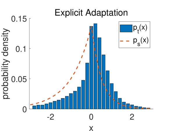
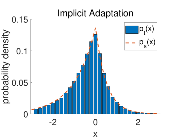
Figure 2: (a) Explicit mass adaptation can lead to wrong time averaged distribution; (b) Implicit mass adaptation produces the correct time averaged distribution.

Our QHMC method employs the implicit mass adaptation. The benefits of this implicit method will be theoretically justified in Section 4. Here we first make the aforementioned intuitions more rigorous by proposing Theorem 4.

Theorem 4

Denote $\mathbf{z}=(\mathbf{x},\mathbf{q})$, and consider the trajectory $\mathbf{z}(t)$ described by the dynamics (17):

$$d\begin{pmatrix}\mathbf{x}\\ \mathbf{q}\end{pmatrix}=dt\begin{pmatrix}\mathbf{A}(\mathbf{z},t)&0\\ 0&\mathbf{A}(\mathbf{z},t)\end{pmatrix}\begin{pmatrix}\mathbf{q}\\ -\nabla U(\mathbf{x})\end{pmatrix}$$ (17)

The only difference between Eq. (17) and Eq. (7) is that $A(\mathbf{z},t)$ replaces $A(t)$. The time-averaged distribution of the particle can be defined as

$$p_{t}(\mathbf{z})=\underset{T\to\infty}{{\rm lim}}\frac{1}{T}\int_{0}^{T}\delta(\mathbf{z}(t)-\mathbf{z})dt$$ (18)

We restrict our discussions to the case $\mathbf{A}(\mathbf{z},t)=a(\mathbf{z},t)\mathbf{I}$. We denote $p(\mathbf{z}|{\cal D})=p(\mathbf{x}|{\cal D})p(\mathbf{q})=p(\mathbf{x}|{\cal D}){\rm exp}(-\mathbf{q}^{T}\mathbf{q}/2)$. For the special case (implicit mass adaptation) $a(\mathbf{z},t)=a(t)$, we have $p_{t}(\mathbf{z})=p(\mathbf{z}|{\cal D})$. However, $p_{t}(\mathbf{z})\neq p(\mathbf{z}|{\cal D})$ for the general case (in an explicit mass adaptation) $a(\mathbf{z},t)\neq a(t)$.

Proof  Our goal is to calculate $p_{t}({\mathbf{z}})$ and compare it with $p(\mathbf{z}|{\cal D})$. The key idea of proof includes two steps:

• Step 1: Change the time variable from $t$ to $t^{\prime}$ and define $p_{t^{\prime}}(\mathbf{z})$. We find $p_{t^{\prime}}(\mathbf{z})=p(\mathbf{z}|D)$.

• Step 2: Establish the relation between $p_{t}(\mathbf{z})$ and $p_{t^{\prime}}(\mathbf{z})$. We find $p_{t}(\mathbf{z})\propto E_{t}(\frac{1}{a(\mathbf{z},t)})p_{t^{\prime}}(\mathbf{z})$.

Step 1: In Eq. (17) we can define a new time variable $t^{\prime}$ such that $dt^{\prime}=a(\mathbf{z},t)dt$, and rewrite the trajectory $\mathbf{z}(t)$ as $\mathbf{z}^{\prime}(t^{\prime})$. With the new time variable $t^{\prime}$, the original time-varying Eq. (17) becomes the standard HMC dynamics in (1). Therefore, we have $p_{t^{\prime}}(\mathbf{z})=p(\mathbf{z}|{\cal D})$ where $p_{t^{\prime}}(\mathbf{z})$ is defined as

$$p_{t^{\prime}}(\mathbf{z})=\underset{T^{\prime}\to\infty}{{\rm lim}}\frac{1}{T^{\prime}}\int_{0}^{T^{\prime}}\delta(\mathbf{z}^{\prime}(t^{\prime})-\mathbf{z})dt^{\prime}.$$ (19)

Step 2: First we note

$$\int_{0}^{T}\delta(\mathbf{z}(t)-\mathbf{z})dt=\sum_{i=1}^{N_{T}(\mathbf{z})}\frac{1}{|\frac{d\mathbf{z}}{dt}(t_{i})|}\bigg{|}_{\mathbf{z}(t_{i})=\mathbf{z}}$$ (20)

where $N_{T}(\mathbf{z})$ counts the number of $t_{i}\leq T$ where $\mathbf{z}(t_{i})=\mathbf{z}$. Consequently, both $p_{t}(\mathbf{z})$ and $p_{t^{\prime}}(\mathbf{z})$ can be rewritten as

$$p_{t}(\mathbf{z})=\underset{T\to\infty}{{\rm lim}}\frac{1}{T}\sum_{i=1}^{N_{T}(\mathbf{z})}\frac{1}{|\frac{d\mathbf{z}}{dt}(t_{i})|}\bigg{|}_{\mathbf{z}(t_{i})=\mathbf{z}},$$ (21)

$$p_{t^{\prime}}(\mathbf{z})=\underset{T^{\prime}\to\infty}{{\rm lim}}\frac{1}{T^{\prime}}\sum_{i=1}^{N^{\prime}_{T^{\prime}}(\mathbf{z})}\frac{1}{|\frac{d\mathbf{z}^{\prime}}{dt^{\prime}}(t^{\prime}_{i})|}\bigg{|}_{\mathbf{z}^{\prime}(t^{\prime}_{i})=\mathbf{z}}.$$ (22)

We further note

$$\bigg{|}\frac{d\mathbf{z}}{dt}(t_{i})\bigg{|}=\frac{dt^{\prime}_{i}}{dt_{i}}\bigg{|}\frac{d\mathbf{z}^{\prime}}{dt^{\prime}}(t^{\prime}_{i})\bigg{|}=a(\mathbf{z}(t_{i}),t_{i})\bigg{|}\frac{d\mathbf{z}^{\prime}}{dt^{\prime}}(t^{\prime}_{i})\bigg{|}.$$ (23)

Combining Eq. (21), (22) and (23), we have

$$p_{t}(\mathbf{z})=\underset{T^{\prime}\to\infty}{{\rm lim}}\frac{1}{T^{\prime}}\sum_{i=1}^{N^{\prime}_{T^{\prime}}(\mathbf{z})}\frac{1}{|\frac{d\mathbf{z}^{\prime}}{dt^{\prime}}(t^{\prime}_{i})|}\times\frac{1}{a(\mathbf{z},t_{i})}\bigg{|}_{\mathbf{z}^{\prime}(t^{\prime}_{i})=\mathbf{z}}\propto E_{t}(\frac{1}{a(\mathbf{z},t)})p_{t^{\prime}}(\mathbf{z})=E_{t}(\frac{1}{a(\mathbf{z},t)})p(\mathbf{z}|{\cal D})$$ (24)

Where the last equality holds due to $p_{t^{\prime}}(\mathbf{z})=p(\mathbf{z}|{\cal D})$. When $a(\mathbf{z},t)=a(t)$, $E_{t}(1/a(\mathbf{z},t))$ is independent of $\mathbf{z}$, and $p_{t}(\mathbf{z})=p(\mathbf{z}|{\cal D})$. Otherwise, $p_{t}(\mathbf{z})\neq p(\mathbf{z}|{\cal D})$ in general when $a(\mathbf{z},t)$ explicitly depends on $\mathbf{z}$.  

In the QHMC algorithm (Alg. 2), $P_{\mathbf{M}}(\mathbf{M})$ is independent of $\mathbf{x}$ or $\mathbf{q}$, therefore the equivalence between $p_{t}(\mathbf{x})$ and $p(\mathbf{x}|{\cal D})$ is justified. In contrast, explicit mass adaptation has $p_{t}(\mathbf{x})\neq p(\mathbf{x}|{\cal D})$ in general. In practical simulations, only a finite number of samples are obtained. The asymptotic distribution error for a general ergodic Markov process has an exponential decay rate (i.e. linear convergence rate) (Bakry et al., 2008), such that $|p_{t}(\mathbf{x})-p(\mathbf{x}|{\cal D})|_{\infty}\leq C\rho^{t}$ where $p_{t}(\mathbf{x})$ is the finite-time sample distribution, $\rho<1$ and $C$ are constant. Therefore, the obtained sample distribution $p_{t}(\mathbf{x})$ can be arbitrarily close to the true posterior distribution $p(\mathbf{x}|{\cal D})$ as long as the stochastic process is simulated for long enough time.

In the current QHMC formulation $\mathbf{M}$ is independent of $\mathbf{x}$. However, it is possible to include a state-dependent mass matrix $\mathbf{M}(\mathbf{x})$ as done in Riemannian HMC (Girolami and Calderhead, 2011) by introduction some correction terms (Ma et al., 2015). This paper focuses on the benefits of QHMC caused by its time-varying mass, therefore we ignore the possible employment of a state-dependent mass matrix.

3.4 Some Remarks

We have some remarks about the general framework of QHMC.

• Some simple cases of QHMC. Although the choice of the mass distribution $P_{\mathbf{M}}(\mathbf{M})$ can be quite general and flexible, a few simple cases turn out to be quite useful in practice: multi-modal, diagonal or scalar mass matrices (corresponding to M-QHMC, D-QHMC or S-QHMC, respectively). Their mass density functions are given below:

  $$\text{\bf M-QHMC}:\mathbf{M}\sim\sum\limits_{i=1}^{k}\alpha_{i}\delta(\mathbf{M}-\mathbf{M}_{i}),\;\text{with}\;\alpha_{i}\geq 0\;\text{and}\;\sum_{i=1}^{k}\alpha_{i}=1$$

  $$\text{\bf D-QHMC}:{\rm log}\;m_{ii}\sim\mathcal{N}(\mu_{m}^{(i)},\sigma_{m}^{(i)2}),\mathbf{M}=\text{diag}(m_{11},\cdots,m_{dd})$$

  $$\text{\bf S-QHMC}:{\rm log}\;m\sim\mathcal{N}(\mu_{m},\sigma_{m}^{2}),\mathbf{M}=m\mathbf{I}.$$

  These simple choices often produce excellent results in practice (see Section 6). The D-QHMC can be regarded as a “quantum" version of preconditioned HMC which has a preconditioner for the mass matrix, and it can improve the sampling performance from an ill-conditioned distribution. The M-QHMC can facilitate sampling from a multi-modal distribution. In both D-QHMC and S-QHMC, the nonzero entries of the mass matrix are sampled from log-normal distributions, which will be justified in Section 4. In our implementation, we often fix $\sigma_{m}=0$ firstly to find the optimal $\mu_{m}$, then we fix $\mu_{m}$ and try different values of $\sigma_{m}$. We find that $\sigma_{m}\in[0.5,3]$ is often an excellent choice. It is worth investigating how to choose $\mu_{m}$ and $\sigma_{m}$ in a more rigorous and automatic way in the future.

• Differences between QHMC and randomized HMC (Bou-Rabee and Sanz-Serna, 2017). Randomized HMC is equivalent to S-QHMC which is a special case of QHMC. Our QHMC has a natural theoretical analysis based on the continuous Fokker-Planck equation (as in Theorem 1). In contrast, the randomized HMC allows a continuous description only when the step size approaches zero. Meanwhile, the parameterizations of randomized HMC and our QHMC are entirely different. Randomized HMC intuitively chooses the exponential form $t\sim\mathrm{exp}(-t/\tau)$ inspired from thermodynamics. This exponential form contains the characteristic time $\tau$, indicating that the sampled time can barely differ from $\tau$ in magnitudes. In contrast, the log-normal parameterization of QHMC allows the mass samples to spread in wide ranges (across multiple magnitudes). This novel parameterization leads to the superior performance of QHMC on the spiky examples in Section 6.

• Possible combinations of QHMC with other advanced techniques. The QHMC method has almost zero extra costs compared with the standard HMC: one only needs to re-sample the mass matrix $\mathbf{M}$ from distribution $P_{\mathbf{M}}(\mathbf{M})$ before performing each standard HMC simulation path. Due to the ease of implementation, QHMC may be easily combined with other techniques, such as the Riemannian manifold method (Girolami and Calderhead, 2011), the continuous tempering technique (Graham and Storkey, 2017) and/or the “no U-Turn” sampler (Hoffman and Gelman, 2014). The M-QHMC implementation may be further improved by combining it with the techniques in continuous tempering HMC (Graham and Storkey, 2017), magnetic HMC (Tripuraneni et al., 2017) and/or wormhole HMC (Lan et al., 2014).

4 Implicit Mass Adaption in QHMC

The mass matrix is set as a positive definite random matrix in QHMC. In this section, we explain how this treatment can benefit the Bayesian sampling in various scenarios.

4.1 Light Particles for Handling Smooth Energy Functions

While using heavy particles (and small step size) can produce more accurate simulation results and higher acceptance rates of a Hamiltonian dynamics, the simulation suffers from random walking behavior and low mixing rates. Here we show that the mass should be appropriately small in order to sample a distribution in a broad region when the associated energy function is very smooth.

We consider a continuous energy function $U(\mathbf{x})$ in $\mathbf{x}\in\mathbb{R}^{d}$ and with $\beta$-smoothness:

$$||\nabla U(\mathbf{x})-\nabla U(\mathbf{y})||_{2}\leq\beta||\mathbf{x}-\mathbf{y}||_{2}$$ (25)

and an HMC implementation with the leapfrog scheme :

$$\mathbf{x}_{n+1} =\mathbf{x}_{n}+\epsilon\mathbf{M}^{-1}\mathbf{q}_{n}$$ (26)

$$\mathbf{q}_{n+1} =\mathbf{q}_{n}-\epsilon\nabla U(\mathbf{x}_{n+1}).$$

In the following, we qualitatively measure the random walking effects with different choices of mass parameters. We first investigate a quadratic energy function in Lemma 5.

Lemma 5

For the quadratic energy function $U(\mathbf{x})=\frac{1}{2}\mathbf{x}^{T}\mathbf{A}\mathbf{x}$ (with $\mathbf{A}$ being symmetric), the discrete dynamical system in Eq. (26) has bounded trajectories if and only if $\mathbf{M}\succ\frac{\epsilon^{2}}{4}\mathbf{A}\succ\mathbf{0}$. Here for two symmetric matrices $\mathbf{A},\mathbf{B}$ the inequality $\mathbf{A}\succ\mathbf{B}$ means $\mathbf{A}-\mathbf{B}$ is positive definite.

Proof  By eliminating $\mathbf{q}_{n}$ in (26) we have the second-order recurrence relation:

$$\mathbf{x}_{n+2}-2\mathbf{x}_{n+1}+\mathbf{x}_{n}+\epsilon^{2}\mathbf{M}^{-1}\nabla U(\mathbf{x}_{n+1})=0.$$ (27)

Because $U(\mathbf{x})=\frac{1}{2}\mathbf{x}^{T}\mathbf{A}\mathbf{x}$, the Eq. (27) becomes

$$\mathbf{x}_{n+2}+(\epsilon^{2}\mathbf{M}^{-1}\mathbf{A}-2\mathbf{I})\mathbf{x}_{n+1}+\mathbf{x}_{n}=0$$ (28)

According to Sylvester’s law of inertia, the spectrum of $\mathbf{M}^{-1}\mathbf{A}$ is identical to the spectrum of $\mathbf{M}^{-\frac{1}{2}}\mathbf{A}\mathbf{M}^{-\frac{1}{2}}$, which is symmetric and hence contain only real eigenvalues. Eq. (28) is bounded if and only if

$$2\mathbf{I}\succ\epsilon^{2}\mathbf{M}^{-1}\mathbf{A}-2\mathbf{I}\succ-2\mathbf{I}$$ (29)

which is equivalent to $\mathbf{M}\succ\frac{\epsilon^{2}}{4}\mathbf{A}\succ\mathbf{0}$.  

We provide a few remarks here. Firstly, the inequality $\frac{\epsilon^{2}}{4}\mathbf{A}\succ\mathbf{0}$ implies that $\mathbf{A}$ should be positive definite, otherwise the quadratic potential function does not have a lower bound and cannot “trap" a particles in a bounded region. Secondly, the first inequality implies that the mass matrix should have large eigenvalues to make the trajectories bounded, which corresponds to a heavy particle moving slowly in $\mathbf{x}$ space.

Next we consider a more general smooth and continuous energy function.

Theorem 6

Assume $U(\mathbf{x})$ is a differentiable and continuous energy function with $\beta$-smoothness. Denote the smallest eigenvalue of $\mathbf{M}$ as $m_{min}>0$ and assume it satisfies $m_{min}>\frac{\beta\epsilon^{2}}{6}$. Without loss of generality we assume $\nabla U(\mathbf{x}^{*})=0$ for $\mathbf{x}^{*}=\mathbf{0}$, and we denote $\mathbf{C}=(\frac{\beta\epsilon^{2}}{2}\mathbf{M}^{-1}-1)$. Lemma 5 implies that the sequence $\{\mathbf{x}_{n}^{*}\}$ generated by $\mathbf{x}_{n+2}^{*}+\mathbf{C}\mathbf{x}_{n+1}^{*}+\mathbf{x}_{n}^{*}=0$ is bounded, i.e. $||\mathbf{x}_{n}^{*}||_{2}<\Delta_{0}$. There exist constants $A$ and $\Delta$, such that $||\mathbf{x}_{n}||_{2}<\Delta$ for all $\mathbf{x}_{n}(n<N_{0})$ generated by Eq. (27). Here $A$ only depends on the initial condition $\mathbf{x}_{0}$, and $N_{0}$ is given by

$$N_{0}=\mathrm{log}_{\lambda}(\frac{\Delta}{A\Delta_{0}}),\lambda=4+\sqrt{17}$$ (30)

Proof 

Given the $\beta$-smoothness condition, we have $||\nabla U(\mathbf{x})-\nabla U(\mathbf{x}^{*})||_{2}\leq\beta||\mathbf{x}-\mathbf{x}^{*}||_{2}$ thus $||\nabla U(\mathbf{x})||\leq\beta||\mathbf{x}||_{2}$. The sequences $\{\mathbf{x}_{n}^{*}\}$ and $\{\mathbf{x}_{n}\}$ are obtained as

$$\begin{split}\mathbf{x}_{n+2}^{*}&=-\mathbf{C}\mathbf{x}_{n+1}^{*}-\mathbf{x}_{n}^{*},\\ \mathbf{x}_{n+2}&=-(\epsilon^{2}\mathbf{M}^{-1}\nabla U(\mathbf{x}_{n+1})-2\mathbf{x}_{n+1})-\mathbf{x}_{n}.\end{split}$$ (31)

Taking the difference between the above two equations we get

$$\begin{split}\mathbf{x}_{n+2}&=(\mathbf{C}\mathbf{x}_{n+1}^{*}+\mathbf{x}_{n}^{*}+\mathbf{x}_{n+2}^{*})-(\epsilon^{2}\mathbf{M}^{-1}\nabla U(\mathbf{x}_{n+1})-2\mathbf{x}_{n+1})-\mathbf{x}_{n}.\end{split}$$ (32)

Denote $\Delta_{n}=||\mathbf{x}_{n}||_{2}$ we have

$$\begin{split}\Delta_{n+2}=||\mathbf{x}_{n+2}||_{2}&\leq||\mathbf{C}\mathbf{x}_{n+1}^{*}+\mathbf{x}_{n}^{*}+\mathbf{x}_{n+2}^{*}||_{2}+\epsilon^{2}||\mathbf{M}^{-1}||_{2}\cdot||\nabla U(\mathbf{x}_{n+1})||_{2}+2||\mathbf{x}_{n+1}||_{2}+||\mathbf{x}_{n}||_{2}\\ &\leq(\lambda_{max}(\mathbf{C})+2)\Delta_{0}+(\frac{\epsilon^{2}\beta}{m_{min}}+2)\Delta_{n+1}+\Delta_{n}<4\Delta_{0}+8\Delta_{n+1}+\Delta_{n}.\end{split}$$ (33)

In the extreme case, $\Delta_{n}$ grows exponentially as $\lambda^{n}$ where $\lambda=4+\sqrt{17}$. Therefore, there should exist a constant $A$ which only depends on the initial conditions, satisfying that

$$\Delta_{n}<A\Delta_{0}\lambda^{n}$$ (34)

By enforcing $A\Delta_{0}\lambda^{n}<\Delta$ for all $n<N_{0}$, we immediately have Eq. (30).  

Following Theorem 6, now we provide a necessary condition for efficiently sampling the posterior density associated with a smooth energy function.

Corollary 7

A sampler can explore the smooth energy function efficiently, if it can find a path from $||\mathbf{x}_{0}||_{2}\leq\Delta_{0}$ to $||\mathbf{x}_{i}||_{2}\geq\Delta$ with no more than $N_{0}$ steps. A necessary condition is

$$m_{min}\leq\frac{\beta\epsilon^{2}}{6}$$ (35)

This implies that the sampler cannot explore the energy function efficiently if the mass is above a certain bound, which is linear with respect to $\beta$.

4.2 Time-Varying Mass for Handling Spiky Distribution

Next we explain how our proposed choice of mass (the log-normal parameterization) can help sample a spiky distribution. Here “spiky" means a distribution whose energy function $U(\mathbf{x})$ has a very large (or even infinite) gradient around some points. Fig. 3 left shows an energy function $U(x)$ with a large gradient at $x=0$. A representative family of spiky distributions is ${\rm exp}\left(-\lambda\|\mathbf{x}\|_{p}^{p}\right)$ with $p\in(0,1]$, which is widely used as a prior density for sparse modeling and model selection (Armagan, 2009; Huang et al., 2008; Donoho et al., 2006; Xu et al., 2010; Zhao et al., 2014; Huang et al., 2008). Here the $\ell_{p}$ norm is defined in a loose sense as $||\mathbf{x}||_{p}=(\sum_{i=1}^{d}|x_{i}|^{p})^{\frac{1}{p}}$. As shown in Fig. 3 middle, $\|\mathbf{x}\|_{p}^{p}$ is non-convex and has divergent gradients around $x=0$ when $0<p<1$, causing troubles in traditional HMC samplers. Sampling from such a spiky distribution is a challenging task in Bayesian learning (Chaari et al., 2016, 2017).

The Hamiltonian dynamical system (1) becomes stiff if the energy function $U(\mathbf{x})$ has a large gradient at some points. This issue can cause unstable numerical simulations. A naive idea is to adapt the step size based on the local gradient $\nabla U(\mathbf{x})$. Unfortunately, this explicit step-size tuning is equivalent to using a state-dependent time modifier $a(\mathbf{z},t)$, and will produce a wrong time-averaged distribution $p_{t}(\mathbf{x})\neq p(\mathbf{x}|{\cal D})$, as proved in Theorem 4. In contrast, the implicit and stochastic mass adaptation in our QHMC is equivalent to using a state-independent time modifier $a(t)$, and it ensures the produced time-averaged distribution converging to the desired posterior density $p(\mathbf{x}|{\cal D})$.

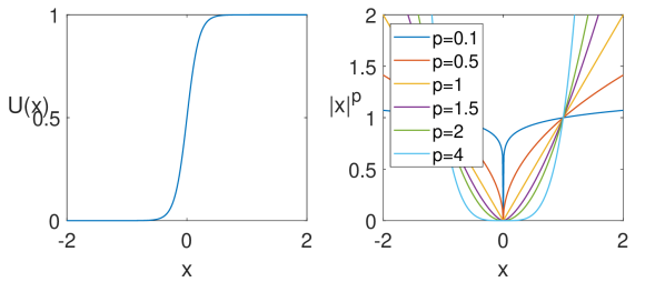
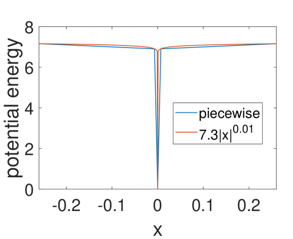
Figure 3: Left: a spiky potential energy function with a very large gradient around $x=0$. Middle: $\|x\|_{p}^{p}$ for various values of $p$. When $p$ tends to zero, $\|x\|_{p}$ becomes an indicator function, which is 0 for $x=0$ and 1 elsewhere. The gradients tend to infinity around $x=0$ for $0<p<1$. Right: the spiky potential function $7.3|x|^{0.01}$ can be approximated by the piecewise linear function in Eq. (36).

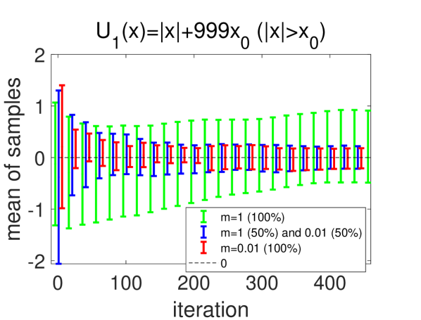
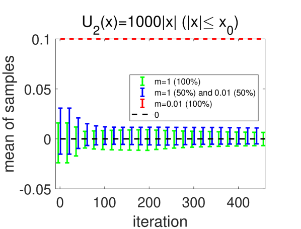
Figure 4: The performance of HMC and QHMC. QHMC uses a random mass with distribution $p_{m}(m)=\frac{1}{2}(\delta(m-1)+\delta(m-0.01))$. (a) Result for the smooth function $U_{1}(x)=|x|+999x_{0}$ where QHMC behaves similarly to HMC with $m=1$ and significantly outperforms HMC with $m=0.01$. (b) Results for the spiky function $U_{2}(x)=1000|x|$, where QHMC behaves similarly to HMC with $m=0.01$ and significantly outperforms HMC with $m=1$.

The advantage of the implicit adaptation strategy in QHMC can be illustrated with a toy spiky distribution with the following potential energy function $U(x)$:

$$U(x)=\left\{\begin{array}[]{lc}U_{1}(x)=|x|+999x_{0}&{\rm if}\;|x|>x_{0},\\ U_{2}(x)=1000|x|&{\rm if}\;|x|\leq x_{0}.\par\end{array}\right.$$ (36)

Here $U(x)$ can be a simple yet good approximation to an $\ell_{p}$ function, as shown on the right of Fig. 3. The spiky and smooth region of $U(x)$ is separated by $-x_{0}$ and $x_{0}$. We care if both regions can be sampled accurately. When $x_{0}={\rm log}(1001)/1000$, the probability of $x$ being located in either region is 0.5, therefore $U_{1}(x)$ and $U_{2}(x)$ are equally important for sampling and we study them independently. Because $U_{1}(x)$ and $U_{2}(x)$ are both symmetric, their associated mean values should be zero, and we measure the numerical performance of a sampler by estimating the error bars obtained from 20 independent experiments. Suppose that we have two mass choices in HMC: $m=1$ or $m=0.01$. In QHMC, we adapt the mass implicitly by allowing $m=1$ and $m=0.01$ with an equal probability. Because $U_{1}(x)=|x|+999x_{0}\ (|x|>x_{0})$ is very smooth, a small mass $m=0.01$ is preferred, as shown in Fig. 4 (a). Although QHMC slightly underperforms the HMC implemented with $m=0.01$, it significantly outperforms the HMC implemented with $m=1$. On the other hand, $U_{2}(x)=1000|x|$ has a very large gradient, therefore a relatively large mass $m=1$ is preferred, as shown in Fig. 4 (b). Similarly, QHMC has slightly worse performance than the HMC implemented with $m=1$, but it performs much better than the HMC implemented with $m=0.01$. In summary, the HMC cannot explore efficiently $U_{1}$ and $U_{2}$ simultaneously with a fixed mass, however our QHMC with an implicit mass adaptation can have excellent performance in both regions.

Remark: Adapting Mass in an Exponential Scale. Corollary 7 implies that one needs to choose a small mass $m\leq\frac{\beta\epsilon^{2}}{6}$ to efficiently explore a potential energy of $\beta$-smoothness. Although $\ell_{p}(0<p<1)$ function has no global $\beta$-smoothness , one can define $\beta$ locally. In the example above, for $x>x_{0}$ or $x<-x_{0}$, $\beta=1$; for $-x_{0}<x<x_{0}$, $\beta=1000$. The wide spread of $\beta$ from 1 to 1000 justifies our choice of a widespread mass distribution as ${\rm log}m\sim{\cal N}(\mu_{m},\sigma_{m}^{2})$ in Alg. 2. In order to adapt to widespread $\beta$, we should adapt $m$ in an exponential scale rather than in a linear scale.

4.3 Explore Multimodal Energy Functions: Quantum Tunneling Effects

Finally, we show that the random mass distribution can help sample a multimodal distribution because it can manifest the “quantum tunneling" effect.

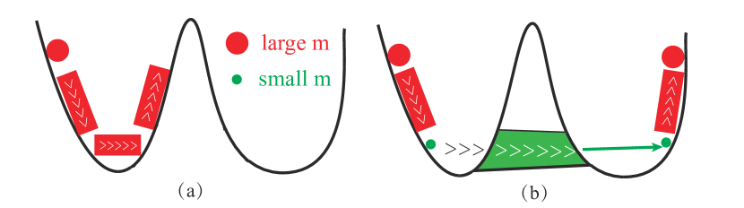
Figure 5: The “quantum tunneling" effects for QHMC. (a) In HMC, a relatively large mass (equivalently, small step size) is chosen to guarantee accurate Hamiltonian simulations. However, the particle can be trapped within one well. (b) In QHMC, the mass is random, and there is chance that one uses a small mass in one path. The light particle has a higher chance to jump to another well through “tunneling".

The “quantum tunneling" effect describes that a microscopic particle may climb over a potential peak even if its total energy is low, which is very different from the case in classical mechanics. In quantum mechanics, a particle should be treated as wave permeable in the whole space rather than a localized object. As a result, the particle (the wave) always has a non-zero probability to climb over the peak. The larger step the particle takes, the more likely a quantum tunneling will happen.

Now we analyze the quantum tunneling effect of our QHMC method in a semi-quantitative way. When a particle has momentum uncertainty $\Delta q$, it should also have a real space uncertainty $\Delta x$ in quantum mechanics such at $\Delta x\Delta q\sim\hbar$, where $\hbar\approx 1.05\times 10^{-34}$ Js is the Plank’s constant and represents the unit of time in the quantum world. In QHMC, the step size $\epsilon$ plays the role of time unit, so we instead have $\Delta x\Delta q\sim\epsilon$. The momentum variable $q$ has a distribution $\propto{\rm exp}(-q^{2}/2m)$ at the thermal equilibrium point, therefore we have momentum uncertainty $\Delta q\sim\sqrt{m}$ and position uncertainty $\Delta x\sim\epsilon/\Delta q=\epsilon/\sqrt{m}$. When $m$ is small the particle is less likely to be trapped in a single well. Fig. 5 (b) shows the intuition of the quantum tunnelling effect.

5 Stochastic-Gradient Implementation

5.1 Quantum Stochastic Gradient Nosé-Hoover Thermostat (QSGNHT)

Similar to HMC, the proposed QHMC method suffers from a high computational cost when the training data size is huge. Consider a machine learning problem with $N$ training samples, the loss (energy) function $U(\mathbf{x})$ is commonly defined as the average loss over all training samples: $U(\mathbf{x})=\frac{1}{N}\sum_{i=1}^{N}U_{i}(\mathbf{x})$, where $U_{i}(\mathbf{x})$ depends only on the $i$-th training sample. Calculating the full gradient $\nabla U(\mathbf{x})$ needs computation over every training sample. Instead, one may replace the true loss with a stochastic estimation $\tilde{U}(\mathbf{x})$, and the stochastic gradient is computed efficiently with only a small batch of samples $\nabla\tilde{U}(\mathbf{x})=\frac{1}{b}\sum_{i=1}^{b}\nabla U_{i}(\mathbf{x})$. Here $b$ is called the batch size. However, the mini-batch estimation of gradients will introduce extra noise. According to the central limit theorem, we can approximate the stochastic gradient as the true gradient plus a Gaussian noise with covariance $V(\mathbf{x})$: $\nabla\tilde{U}(\mathbf{x})\approx\nabla U(\mathbf{x})+{\cal N}(0,\mathbf{V}(\mathbf{x}))$, if $b$ is much smaller than $N$ but still relatively large.

However, such a naive stochastic gradient implementation can result in incorrect steady distribution, and one can add a friction term to compensate for the extra noise in a stochastic-gradient HMC (Chen et al., 2014). Different from the friction formulation in (Chen et al., 2014), we utilize the thermostat technique (Ding et al., 2014; Leimkuhler and Reich, 2009) to correct the steady distribution. Specifically, we treat the gradient uncertainty term $\mathbf{V}(\mathbf{x})$ as a noise with an unknown magnitude, and use the Nosé-Hoover thermostat to avoid the explicit estimation of this gradient noise term. The resulting update rule for $(\mathbf{x},\mathbf{q},\xi)$ is shown in Eq. (37) with step size $\epsilon$:

$$\left\{\begin{aligned} &\mathbf{x}_{i+1}\leftarrow\ \mathbf{x}_{i}+\epsilon\mathbf{M}_{t}^{-1}\mathbf{q}_{i}\quad\\ &\mathbf{q}_{i+1}\leftarrow\ \mathbf{q}_{i}-\epsilon\nabla\tilde{U}(\mathbf{x}_{i+1})-\epsilon\xi_{i}\mathbf{q}_{i}+\sqrt{2A}{\cal N}(0,\epsilon\mathbf{I})\\ &\xi_{i+1}\leftarrow\ \xi_{i}+\frac{\epsilon}{m_{\mu}}(\mathbf{q}_{i+1}^{T}\mathbf{M}_{t}^{-1}\mathbf{q}_{i+1}-{\rm Tr}(\mathbf{M}_{t}^{-1}))\end{aligned}\right.$$ (37)

where $\mathbf{M}_{t}$ refers to the mass matrix used for the $t$-th path, $i=1,2,\cdots,L$ refers to the index of steps in each path. $A$ indicates the magnitude of injected noise, $m_{\mu}$ is the thermal mass term, $d_{0}$ is the dimension of $\mathbf{x}$, and $T$ is in the definition of the energy function $U(x)=-T{\rm log}(p(\mathbf{x}|{\cal D}))$. We set $m_{\mu}=1$ (like in  (Ma et al., 2015)), $A=1$ and $T=1$. We refer to the proposed method with thermostat as quantum stochastic gradient Nosé-Hoover thermostat (QSGNHT). The algorithm flow of QSGNHT is shown in Alg. 3.

Input: starting point $x_{0}$, step size $\epsilon$, simulation steps $L$, mass distribution parameters $\mu_{m}$ and $\sigma_{m}$, thermal mass $m_{\mu}$, batch size $b$, dimension of $\mathbf{x}$ is $d$, temperature $T$, diffusion strength $A$.

for $t=1,2,\cdots$ do

       Randomly select $b$ samples out of the $N$ training samples and compute $\tilde{U}(\mathbf{x})=\frac{1}{b}\sum_{i=1}^{b}U_{i}(\mathbf{x})$;

       Resample $\mathbf{M}_{t}\sim P_{\mathbf{M}}(\mathbf{M})$ , and resample $\mathbf{q}\sim{\cal N}(0,\mathbf{M}_{t})$;

       ($\mathbf{x}_{0},\mathbf{q}_{0}$)=($\mathbf{x}^{(t)},\mathbf{q}^{(t)}$);

       Simulate dynamics based on Eq. (37);

       $\mathbf{q}_{0}\leftarrow\mathbf{q}_{0}-\frac{\epsilon}{2}\nabla\tilde{U}(\mathbf{x}_{0})$;

       for $i=1,\cdots,L-1$ do

             $\mathbf{x}_{i+1}\leftarrow\ \mathbf{x}_{i}+\epsilon\mathbf{M}_{t}^{-1}\mathbf{q}_{i}$;

             $\mathbf{q}_{i+1}\leftarrow\ \mathbf{q}_{i}-\epsilon\nabla\tilde{U}(\mathbf{x}_{i+1})-\epsilon\xi_{i}\mathbf{q}_{i}+\sqrt{2A}{\cal N}(0,\epsilon\mathbf{I})$;

             $\xi_{i+1}\leftarrow\ \xi_{i}+\frac{\epsilon}{m_{\mu}}(\mathbf{q}_{i+1}^{T}\mathbf{M}_{t}^{-1}\mathbf{q}_{i+1}-{\rm Tr}(\mathbf{M}_{t}^{-1}))$;

       end for

      $\mathbf{q}_{L}\leftarrow\mathbf{q}_{L}-\frac{\epsilon}{2}\nabla\tilde{U}(\mathbf{x}_{L})$;

       ($\hat{\mathbf{x}},\hat{\mathbf{q}}$)=($\mathbf{x}_{L},\mathbf{q}_{L}$);

       M-H step: $u\sim\mathrm{Uniform[0,1]}$;

       Define $\tilde{H}(\mathbf{x},\mathbf{q})=\tilde{U}(\mathbf{x})+\frac{1}{2}\mathbf{q}^{T}\mathbf{M}_{i}^{-1}\mathbf{q}$;

       $\rho=e^{-\tilde{H}(\hat{\mathbf{x}},\hat{\mathbf{q}})+\tilde{H}(\mathbf{x}^{(t)},\mathbf{q}^{(t)})}$;

       if $u<\mathrm{min}(1,\rho)$ then

            $(\mathbf{x}^{(t+1)},\mathbf{q}^{(t+1)})=(\hat{\mathbf{x}},\hat{\mathbf{q}})$

      else

            $(\mathbf{x}^{(t+1)},\mathbf{q}^{(t+1)})=(\mathbf{x}^{(t)},\mathbf{q}^{(t)})$

       end if

      

end for

Output: $\{\mathbf{x}^{(1)},\mathbf{x}^{(2)},\cdots\}$

Algorithm 3 Quantum Stochastic Gradient Nosé-Hoover Thermostat (QSGNHT)

5.2 Theoretical Analysis based on Stochastic Differential Equation (SDE)

In this subsection, we prove that the QSGNHT implementation in Alg. 3 indeed produces the desired posterior density $p(\mathbf{x}|{\cal D})$. Setting $\mathbf{M}(t)=m(t)\mathbf{I}$, we first provide the continuous-time stochastic differential equation (SDE) for QSGNHT:

$$d\begin{pmatrix}\mathbf{x}\\ \mathbf{q}\\ \xi\end{pmatrix}=dt\begin{pmatrix}\mathbf{M}(t)^{-1}\mathbf{q}\\ -\nabla U(\mathbf{x})-\xi\mathbf{q}+{\cal N}(0,\mathbf{V}(\mathbf{x}))\epsilon\\ \frac{1}{m_{\mu}}(\mathbf{q}^{T}\mathbf{M}(t)^{-1}\mathbf{q}-{\rm Tr}(\mathbf{M}(t)^{-1}))\end{pmatrix}+\begin{pmatrix}0\\ \sqrt{2A}d\mathbf{W}(t)\\ 0\end{pmatrix}$$ (38)

where $\epsilon$ is the step size in the discretized dynamics. Before presenting our result in Theorem 10, we review the result for a general continuous-time Markov process in Lemma 8.

Lemma 8

(Theorem 1 in (Ma et al., 2015)) A general continuous-time Markov process can be written as a stochastic differential equation (SDE) in this form:

$$d\mathbf{z}=\mathbf{f}(\mathbf{z})dt+\sqrt{2\mathbf{D}(\mathbf{z})}d\mathbf{W}(t)$$ (39)

where $\mathbf{z}$ can be a general vector and $\mathbf{D}(\mathbf{z})$ represents the magnitude of the Wiener diffusion process. Then, $p_{s}(\mathbf{z})\propto{\rm exp}(-H(\mathbf{z}))$ is a steady distribution of the above SDE if $f(\mathbf{z})$ can be written as:

$$\mathbf{f}(\mathbf{z})=-(\mathbf{D}(\mathbf{z})+\mathbf{Q}(\mathbf{z}))\nabla H(\mathbf{z})+\mathbf{\Gamma}(\mathbf{z}),\quad\mathbf{\Gamma}_{i}(\mathbf{z})=\sum_{i=1}^{d}\frac{\partial}{\partial\mathbf{z}_{j}}(\mathbf{D}_{ij}(\mathbf{z})+\mathbf{Q}_{ij}(\mathbf{z}))$$ (40)

where $H(\mathbf{z})=U(\mathbf{x})+g(\mathbf{x},\mathbf{q})$ is the Hamiltonian of the system, $U(\mathbf{x})=-{\rm log}p(\mathbf{x}|{\cal D})$ is the potential energy, $g(\mathbf{x},\mathbf{q})=\frac{1}{2}\mathbf{q}^{T}\mathbf{M}(t)^{-1}\mathbf{q}/2$ is the kinetic energy, $\mathbf{Q}(z)$ determines the deterministic transverse dynamics, $\mathbf{D}(\mathbf{z})$ is positive semidefinite, and $\mathbf{Q}(\mathbf{z})$ skew-symmetric. The steady distribution $p_{s}(\mathbf{z})$ is unique if $\mathbf{D}(\mathbf{z})$ is positive definite, or if ergodicity  can be shown.

Proof  The proof is based on (Ma et al., 2015). According to Eq. (39) we have a corresponding Fokker-Planck equation to describe the evolution of the probability density:

$$\partial_{t}p(\mathbf{z},t)=-\sum_{i}\frac{\partial}{\partial\mathbf{z}_{i}}(\mathbf{f}_{i}(\mathbf{z})p(\mathbf{z},t))+\sum_{i,j}\frac{\partial^{2}}{\partial\mathbf{z}_{i}\partial\mathbf{z}_{j}}(\mathbf{D}_{ij}(\mathbf{z})p(\mathbf{z},t))$$ (41)

Eq. (41) can be further written in a more compact form:

$$\partial_{t}p(\mathbf{z},t)=\nabla^{T}\cdot([\mathbf{D}(\mathbf{z})+\mathbf{Q}(\mathbf{z})][p(\mathbf{z},t)\nabla H(\mathbf{z})+\nabla p(\mathbf{z},t)])$$ (42)

We are able to verify $p_{s}(\mathbf{x},\mathbf{q},\xi)\propto{\rm exp}(-H(\mathbf{x},\mathbf{q},\xi))$ is invariant under Eq. (41) by calculating $[e^{-H(\mathbf{z})}\nabla H(\mathbf{z})+\nabla e^{-H(\mathbf{z})}]=0$. If the process if ergodic, then the stationary distribution is unique. The ergodicity of the Markov process requires three conditions: (a) irreducibility (b) aperiodicity (c) positive recurrence. Irreducibility and aperiodicity can be guaranteed by non-zero diffusion noises, while positive recurrence is satisfied if $U(\mathbf{x})\to\infty$ when $|\mathbf{x}|\to\infty$.  

Lemma 9

Consider a system described by Eq. (38) but with deterministic constant mass $\mathbf{M}(t)=\mathbf{M}_{0}$, then the steady distribution is unique and proportional to ${\rm exp}(-U(\mathbf{x}))$.

Proof  Compare Eq. (38) with Eq. (39) and (40) we can determine the corresponding Hamiltonian and coefficient matrices $\mathbf{D}$ and $\mathbf{Q}$:

$$H(\mathbf{x},\mathbf{q},\xi)= U(\mathbf{x})+\frac{1}{2}\mathbf{q}^{T}\mathbf{M}_{0}^{-1}\mathbf{q}+\frac{m_{\mu}}{2}(\xi-A-\frac{V(\mathbf{x})\epsilon}{2})^{2}$$ (43)

$$\mathbf{D}(\mathbf{x},\mathbf{q},\xi)=\begin{pmatrix}0&0&0\\ 0&A+\frac{V(\mathbf{x})\epsilon}{2}&0\\ 0&0&0\\ \end{pmatrix}, \quad\mathbf{Q}(\mathbf{x},\mathbf{q},\xi)=\begin{pmatrix}0&-\mathbf{I}&0\\ \mathbf{I}&0&\mathbf{M}_{0}^{-1}\mathbf{q}/m_{\mu}\\ 0&-\mathbf{q}^{T}\mathbf{M}_{0}^{-1}/m_{\mu}&0\\ \end{pmatrix}.$$

Obviously $\mathbf{D}(\mathbf{x},\mathbf{q},\xi)$ is positive semi-definite and $\mathbf{Q}(\mathbf{x},\mathbf{q},\xi)$ is skew-symmetric. By denoting $\mathbf{z}=(\mathbf{x},\mathbf{q},\xi)$, we know that there exists a steady distribution $p_{s}(\mathbf{z})\propto{\rm exp}(-H(\mathbf{z}))={\rm exp}(-U(\mathbf{x})-\frac{1}{2}\mathbf{q}^{T}\mathbf{M}_{0}^{-1}\mathbf{q}-\frac{1}{2}m_{\mu}(\xi-A-\frac{V(\mathbf{x})\epsilon}{2})^{2})$. Due to non-zero diffusion error $A>0$ in the system, $p_{s}(\mathbf{x},\mathbf{q},\xi)$ is the unique steady distribution. Marginalizing over $\mathbf{q}$ and $\xi$, one obtains $p_{s}(\mathbf{x})\propto{\rm exp}(-U(\mathbf{x}))$.  

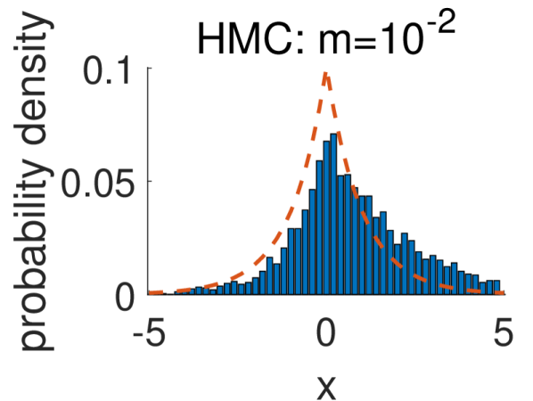
(a)

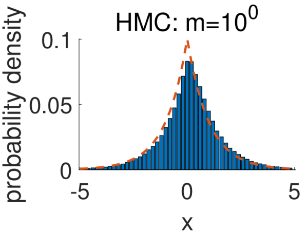
(b)

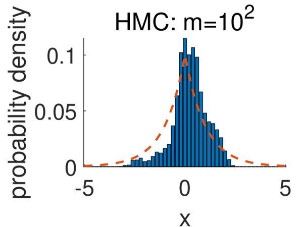
(c)

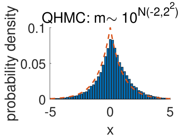
(d)

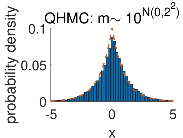
(e)

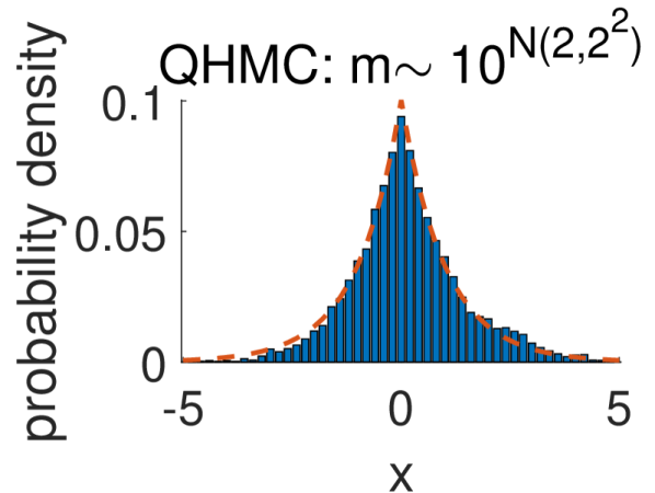
(f)

Figure 6: The results of HMC and QHMC for the energy function $U(x)=|x|$. The red dashed line: true distribution; blue histogram: the probability obtained with 200000 simulation samples. (a)-(c) HMC is sensitive to the choice of mass; (d)-(f) QHMC works well for a large range of mass parameters.

Similar to the second proof of Theorem 1, we have Theorem 10 stated below.

Theorem 10

The Markov process in Eq. (38) has a unique marginal steady distribution $p_{s}(\mathbf{x})\propto{\rm exp}(-U(\mathbf{x}))$.

Proof  From lemma 9 we know that given a constant mass matrix $\mathbf{M}$, we have

$$p_{s}(\mathbf{x},\mathbf{q},\xi|\mathbf{M})\propto{\rm exp}(-U(\mathbf{x})){\rm exp}(-\frac{1}{2}\mathbf{p}^{T}\mathbf{M}^{-1}\mathbf{p}){\rm exp}(-\frac{1}{2}m_{\mu}(\xi-A-\frac{V(\mathbf{x})\epsilon}{2})^{2}).$$ (44)

Employing the Bayes rule $p_{s}(\mathbf{x},\mathbf{q},\xi,\mathbf{M})=p_{s}(\mathbf{x},\mathbf{q},\xi|\mathbf{M})P_{\mathbf{M}}(\mathbf{M})$, and marginalizing the joint distribution over $\mathbf{q},\xi,\mathbf{M}$ we have

$$p_{s}(\mathbf{x})=\int_{\mathbf{q}}\int_{\xi}\int_{\mathbf{M}}\ d\mathbf{q}\ d\xi\ d{\mathbf{M}}\ p_{s}(\mathbf{x},\mathbf{q},\xi,\mathbf{M})\propto{\rm exp}(-U(\mathbf{x})).$$ (45)

 

6 Numerical Experiments and Applications

This section verifies our proposed methods by several synthetic examples and some machine learning tasks such as sparse bridge regression, image denoising, and neural network pruning. Our default implementation of QHMC is the scalar QHMC (i.e., S-QHMC in Section 3.4) unless stated explicitly otherwise. The number of simulation steps and the step size are set as $L=5$ and $\epsilon=0.03$ in QHMC, if not stated explicitly otherwise . Our codes are implemented in MATLAB and Python, and all experiments are run in a computer with 4-core 2.40 GHz CPU and 8.0G memory. All codes are available at https://github.com/KindXiaoming/QHMC.

6.1 Synthetic Examples

6.1.1 One-Dimensional $\ell_{p}$ Norm

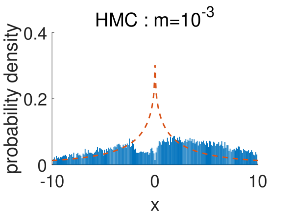
(a)

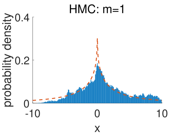
(b)

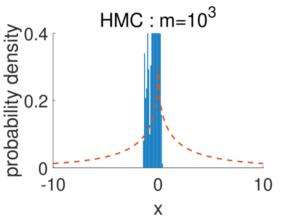
(c)

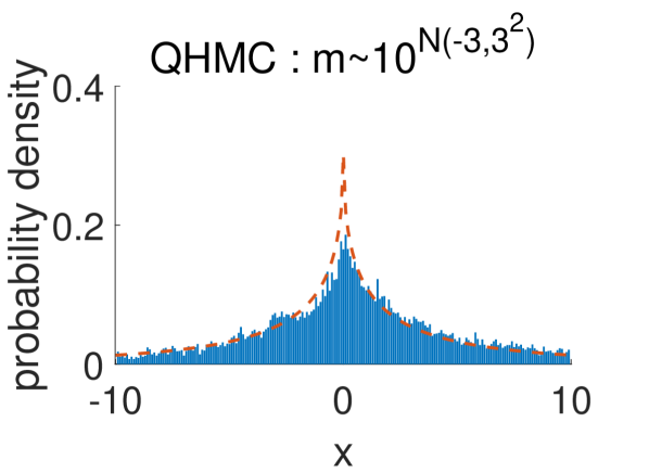
(d)

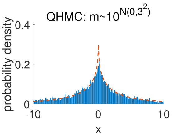
(e)

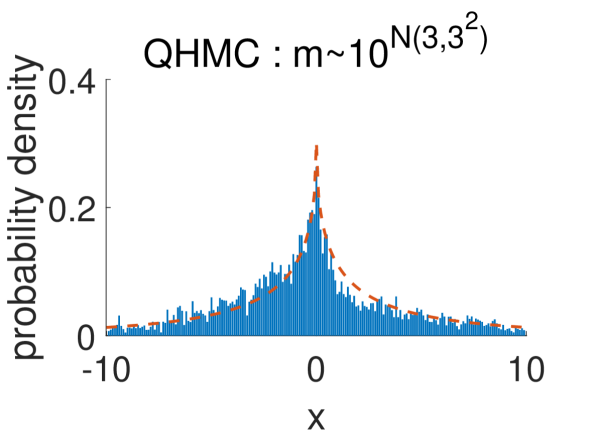
(f)

Figure 7: The performance of HMC and QHMC in sampling ${\rm exp}(-|x|^{1/2})$. Red dashed line: true distribution; blue histogram: simulation result with 50000 samples. HMC is sensitive to the mass parameters, whereas QHMC has excellent performance even if the mass parameters change in a wide range.

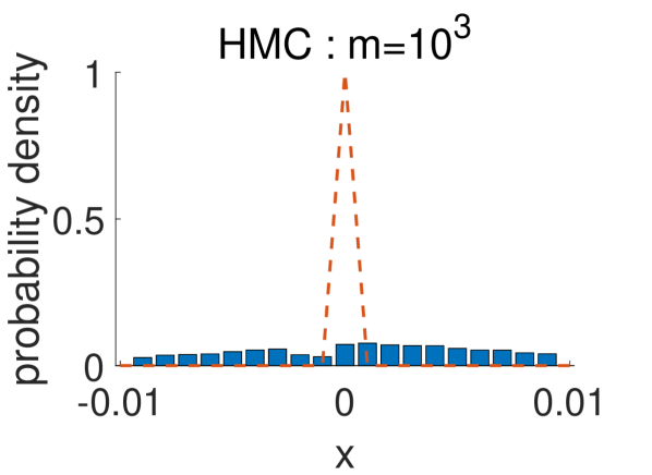
(a)

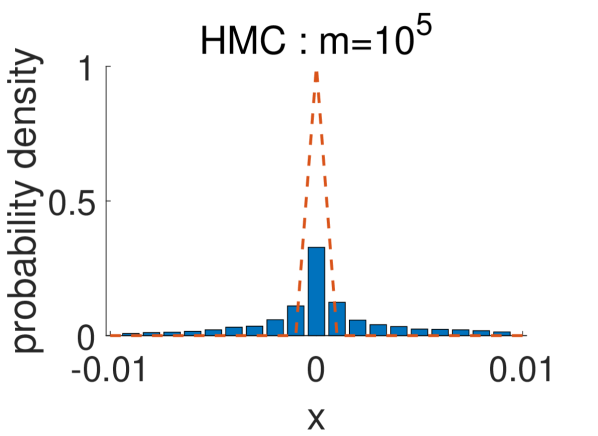
(b)

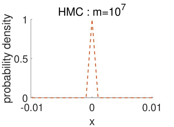
(c)

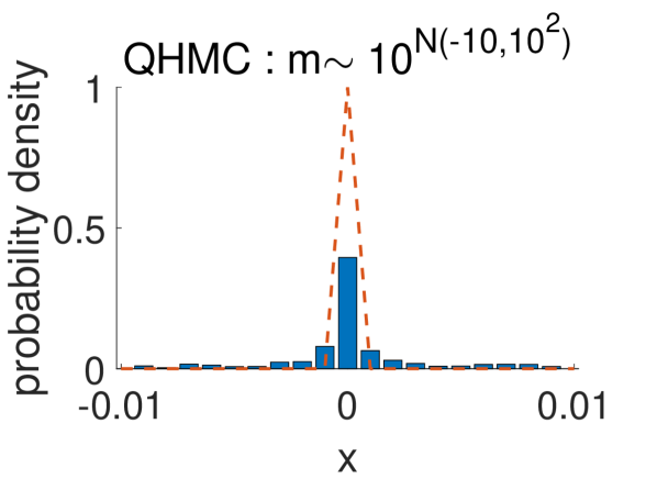
(d)

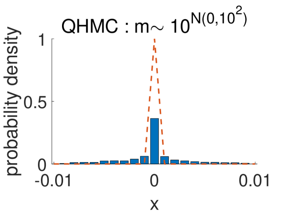
(e)

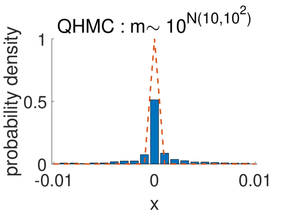
(f)

Figure 8: The results of HMC and QHMC for the energy function $U(x)=20|x|^{1/10}$. The red dashed line is the true distribution, and the blue histogram is the distribution with 50000 simulation samples. (a)-(c): HMC with different mass values; (d)-(f) QHMC results obtained with different distributions for the mass parameter.

The $\ell_{p}$ $(0<p<1)$ norm can be used as a regularizer in an optimization problem for model selection and to enforce model sparsity (Zhao et al., 2014; Xu et al., 2010). In a Bayesian setting, employing an $\ell_{p}$ regularization is equivalent to placing a prior density ${\rm exp}(-\frac{\|\mathbf{x}\|_{p}^{p}}{\tau})$.

In this experiment, we use QHMC to sample from a 1-D distribution $p(x)\propto{\rm exp}(-|x|^{p})$ whose corresponding potential energy function is $U(x)=|x|^{p}$ for $p=\{1,0.5,0.1\}$. We start from $x_{0}=0.1$, which is already in the typical set , therefore the burn-in steps are not needed. The results for $p=1,0.5,0.1$ are presented in Fig. 6 to Fig. 8 respectively. We can see that as $p$ approaches zero, the advantages of QHMC over HMC becomes increasingly significant.

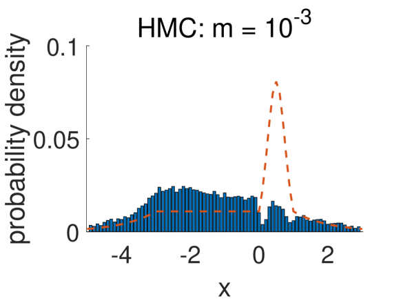
(a)

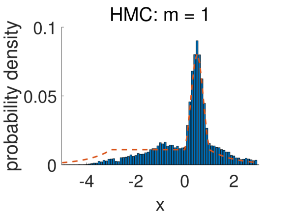
(b)

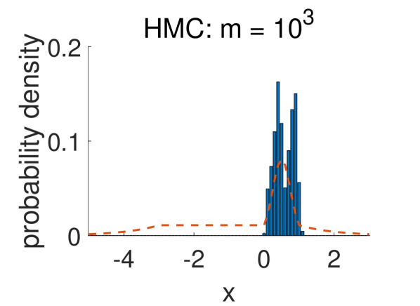
(c)

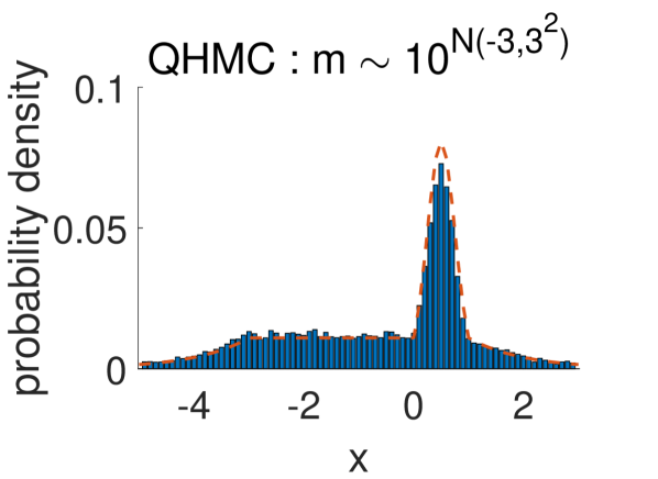
(d)

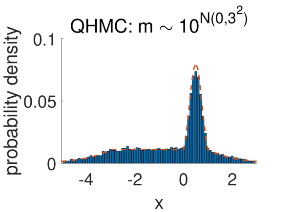
(e)

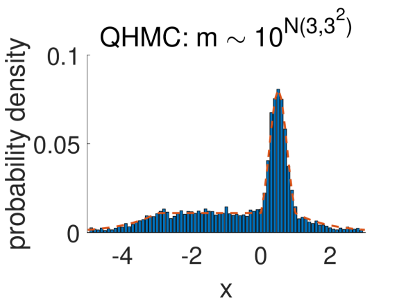
(f)

Figure 9: The spiky+smooth distribution example. We run 50000 paths to get the sample distributions. The ground truth is shown by the dashed red line. It is hard to pick a fixed $m$ in HMC to get accurate results for both the flat smooth region and the spiky region, as shown in (a)–(c). The proposed QHMC can accurately sample the entire target distribution for a wide range of mass distributions, as shown in (d)–(f).

We compare HMC and QHMC implemented with different mass parameters. Take the results of $p=0.5$ as an example (see Fig. 7). In each row, the mass value in HMC is set as the the median mass value of QHMC. Fig. 7 (a)-(c) show that the distribution can be well sampled by HMC only if the mass value is properly chosen. The region around $x=0$ can be hardly explored when the mass value is too small, as shown in Fig. 7 (a). In Fig. 7 (c), the whole distribution cannot be well explored due to the random walk caused by a large mass. However, the proposed QHMC method does not suffer from this issue. As shown in Fig. 7 (d)-(f), the QHMC can produce accurate sample distributions when the median mass value $10^{\mu_{m}}$ changes from $10^{-3}$ to $10^{3}$.

6.1.2 One-Dimensional Distribution with Both Smooth and Spiky Regions

Section 4 states that different mass magnitudes are preferred for smooth and spiky regions. In this example, we consider the following piecewise (non-normalized) potential energy function:

$$U(x)=\left\{\begin{array}[]{lc}-x-3&(x\leq-3)\\ 0&(-3<x\leq 0)\\ 8x(x-1)&(0<x\leq 1)\\ x-1&(x>1).\end{array}\right.$$ (46)

This function is very flat and smooth in the range $[-3,0]$ and very spiky in the interval $[0,1]$.

In order to understand why QHMC outperforms HMC in this synthetic example, we provide a semi-quantitative analysis by introducing the diffusion coefficient $D$ and characteristic length $r_{c}$. We consider the flat energy function $U(x)=0$ for $-3<x\leq 0$. Suppose that we use a fixed step size $\epsilon$ and $L$ leap-frog steps in each simulation path, and that we run $N$ simulation paths. Because $q_{i}(i=1,2,\cdots,N)$ are drawn from a Gaussian distribution, their sum also has a Gaussian distribution with a variance that is $N$ times larger. Suppose the particle starts from $x_{0}=0$, therefore at step $N$ the position of the particle is $x=(\epsilon L/m)\sum_{i=1}^{N}p_{i}$, and it is easy to verify the variance of $x$ is $\overline{x^{2}}=N(\epsilon L)^{2}/m$. We can define the diffusion coefficient $D$ as $\overline{x^{2}}=2DN$ such that $D=(\epsilon L)^{2}/2m\sim 1/m$. Define the characteristic step size as $\epsilon_{c}=\sqrt{\overline{x^{2}}/N}=\sqrt{2D}$. Let $r_{c}$ be the characteristic scale of the smooth region . If the particle can explore the smooth region within $N\sim O(1)$ steps, the characteristic step size $\epsilon_{c}$ and characteristic scale $r_{c}$ should be at the same order, i.e. $D\sim O(\epsilon_{c}^{2})\sim O(r_{c}^{2})$ or equivalently $m\sim O((\epsilon L)^{2}/2r_{c}^{2})$.

We can roughly estimate the optimal mass for the piecewise function. On the one hand, Lemma 5 indicates that the mass should be above $a\epsilon^{2}/4=3.6\times 10^{-3}$ for the spiky region $[0,1]$. On the other hand, based on the discussion above and the characteristic length $r_{c}\sim 3$, we know the optimal mass is $m\sim(\epsilon L)^{2}/2r_{c}^{2}=1.3\times 10^{-3}$ for the smooth region $[-3,0]$. These two requirements cannot be meet simultaneously with a fixed mass as in a standard HMC. As a result, the HMC produces inaccurate distributions for this example, as shown in Fig. 9 (a)-(c).

However, the QHMC can employ a random mass to generate accurate sample distributions in both regions. To demonstrate this, we start from $x_{0}=0$ and run 50000 paths. As shown in Fig. 9 (d)-(e), the QHMC produces accurate distributions with $\mu_{m}$ varying in a wide range.

6.1.3 One-dimensional Multimodal Distribution

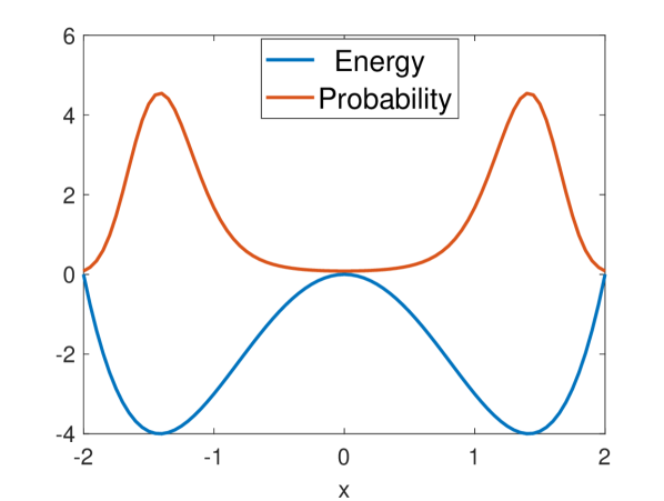
(a)

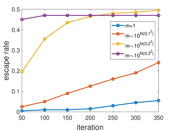
(b)

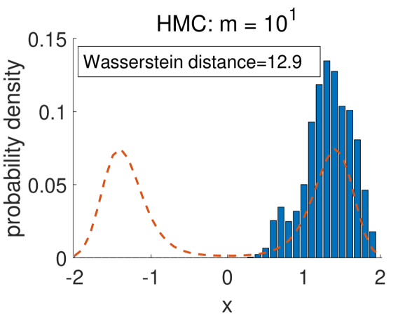
(c)

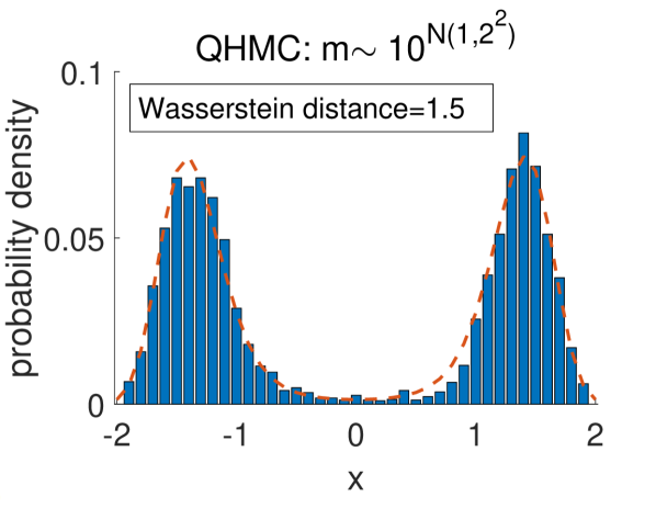
(d)

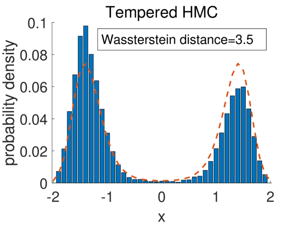
(e)

Figure 10: A double-well example. (a) The potential energy function $U(x)=x^{4}-4x^{2}$ has global minimum at $\pm\sqrt{2}$. We initiate the particle from $x_{0}=\sqrt{2}$ and run the HMC/QHMC sampling. (b) The escape ratio of HMC and QHMC. (c)-(e): sample distributions from HMC, QHMC and tempered HMC, respectively. We test each algorithm for 100 trials, and plot its sampling result with the 20th smallest Wasserstein distance.

This experiment shows the effectiveness of QHMC in sampling from a multimodal distribution, which is explained in Section 4.3.

We consider a double-well posterior distribution $p(x)\propto{\rm exp}(-U(x))$ where the potential energy function $U(x)=x^{4}-4x^{2}$, as shown in Fig. 10 (a). We simulate 200 particles starting from the right minimum point $x_{0}=\sqrt{2}$, and we check if each particle has crossed the peak at $x=0$ after every 50 iterations. If yes, then the particle has successfully escaped from the right well. We report the ratio of particles that have escaped from the right wells after certain iterations in Fig. 10 (b). We observe that a moderate variance $\sigma_{m}\sim 2$ of the log-mass distribution can lead to significantly better performance than simply fixing the mass in standard HMC. We also observe that the particles can escape from the right well more quickly once the log-mass distribution has a larger variance.

We further compare the proposed QHMC algorithm with standard HMC and tempered HMC (Graham and Storkey, 2017). The HMC with tempering is implemented by setting a low temperature $T_{l}=1$ and high temperature $T_{h}=25$ and run a high-temperature step every 30 paths, including 10 paths of burn-in and 20 paths to collect samples. For each method, we run 100 trials of sampling results and sort them by the Wasserstein distance. We show the sample distributions with the 20th smallest Wasserstein distance in Fig. 10 (c)–(e). The QHMC method produces very accurate results due to its quantum tunneling effect. Tempered HMC can produce a multimodal sample distribution, but its Wasserstein distance is larger than that of QHMC.

6.1.4 Ill-Conditioned Gaussian Distribution

In Section 3.4, we proposed two practical parameterizations of QHMC: S-QHMC and D-QHMC. We show for the ill-conditioned Gaussian distribution, D-QHMC can take into account different scalings along each dimension, hence outperforms S-QHMC and randomized HMC significantly.

The Gaussian distribution $p(\mathbf{x})\propto{\rm exp}(-\frac{1}{2}\mathbf{x}^{T}\mathbf{\Sigma}^{-1}\mathbf{x})$ is a well-studied case in sampling problems. The preconditing of mass matrix can help improve sampling performance of ill-conditioned Gaussian distributions and the rule of thumb is $\mathbf{M}^{-1}\sim\mathbf{\Sigma}$ as mentioned in e.g.  (Beskos et al., 2011). We consider an ill-conditioned Gaussian with $\mathbf{\Sigma}=\rm{diag}(100,1)$. The sampler starts from $\mathbf{x}_{0}=\mathbf{0}$ and run 10000 paths to collect samples.

The results are shown in Fig. 11. We compare five methods: (a) standard HMC: $m=0.01$; (b) Randomized HMC: $m=0.01$ and $\tau=0.03$; (c) Riemannian HMC: $\mathbf{M}=0.1\mathbf{\Sigma}^{-1}$; (d) S-QHMC: $\mu_{m}=-2,\sigma_{m}=1$; (e) D-QHMC: $\mu_{m}^{(1)}=-3,\mu_{m}^{(2)}=-1,\sigma_{m}^{(1)}=\sigma_{m}^{(2)}=1$. It is clear that D-QHMC outperforms all other four methods on this example.

(a)

(b)

(c)

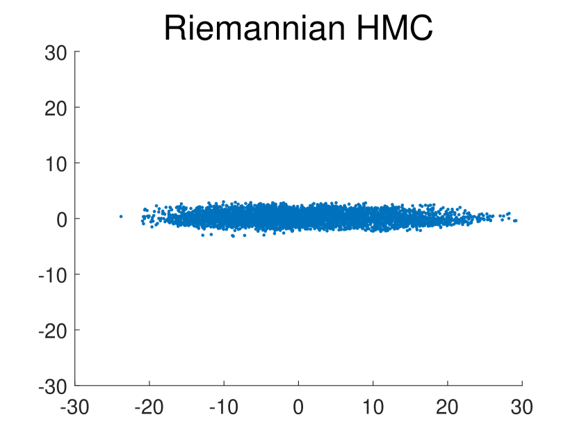
(d)

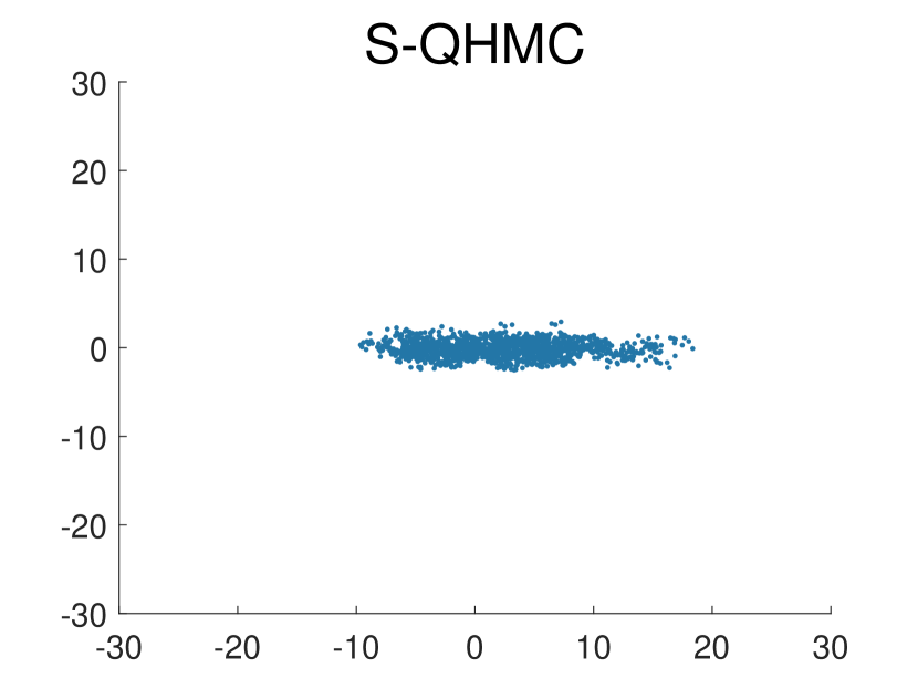
(e)

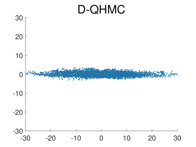
(f)

Figure 11: An ill-conditioned Gaussian distribution. (a) shows the samples drawn from the ground truth. (b)-(f) five methods used to sample the distribution: HMC, randomized HMC, riemannian HMC, S-QHMC and D-QHMC. D-QHMC outperforms S-QHMC and other baselines.

6.1.5 Two-Dimensional Gaussian Mixture Model

In this example, we show how the multi-mode QHMC (i.e., M-QHMC) described Section 3.4 can help sample from a Gaussian-mixture distribution.

We consider the target two-modal distribution:

$$p(\mathbf{x})=p_{1}{\rm exp}(-\frac{1}{2}\mathbf{x}^{T}\mathbf{\Sigma}_{1}^{-1}\mathbf{x})+p_{2}{\rm exp}(-\frac{1}{2}\mathbf{x}^{T}\mathbf{\Sigma}_{2}^{-1}\mathbf{x})$$ (47)

with $p_{1}=p_{2}=\frac{1}{2}$, $\mathbf{\Sigma}_{1}={\rm diag}(1,100)$ and $\mathbf{\Sigma}_{2}={\rm diag}(100,1)$. We intend to compare five sampling methods: (1) baseline HMC with $\mathbf{M}=m\mathbf{I}$ ($m=0.02$); (2) randomized HMC with $m=0.02$ and $\tau=0.03$; (3) Riemannian HMC with $\mathbf{M}=0.1\mathbf{\Sigma}_{1}^{-1}$; (4) D-QHMC with $\mu_{m}^{(1)}=\mu_{m}^{(2)}=-2,\sigma_{m}^{(1)}=\sigma_{m}^{(2)}=1$; (5) M-QHMC with $P_{\mathbf{M}}(\mathbf{M})=\frac{1}{2}\delta(\mathbf{M}-0.1\mathbf{\Sigma}_{1}^{-1})+\frac{1}{2}\delta(\mathbf{M}-0.1\mathbf{\Sigma}_{2}^{-1})$.

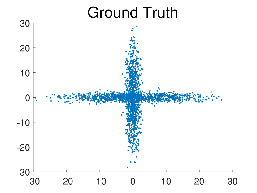
(a)

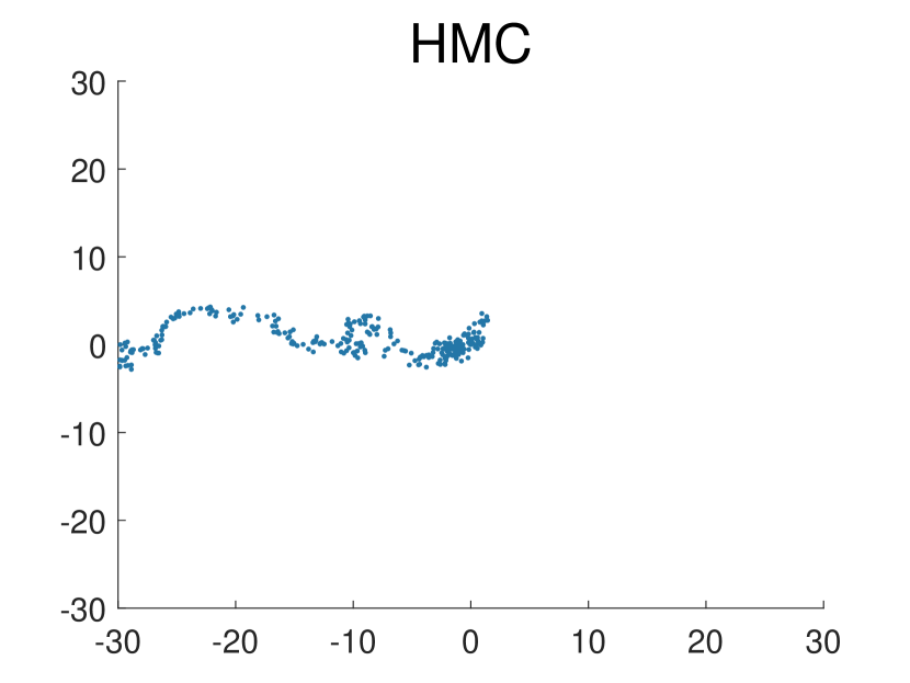
(b)

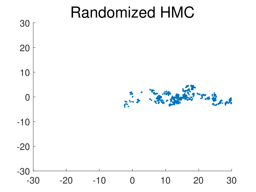
(c)

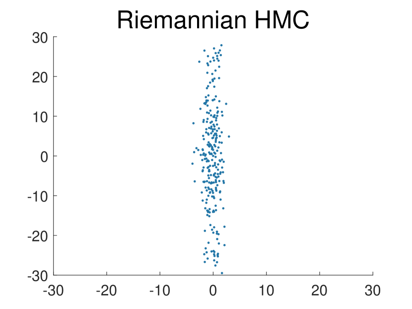
(d)

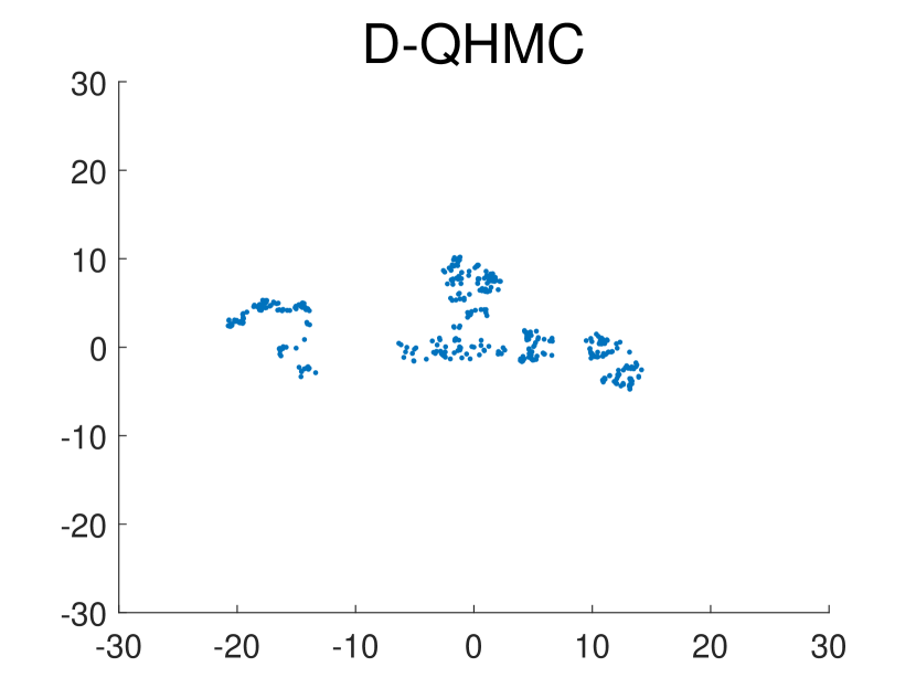
(e)

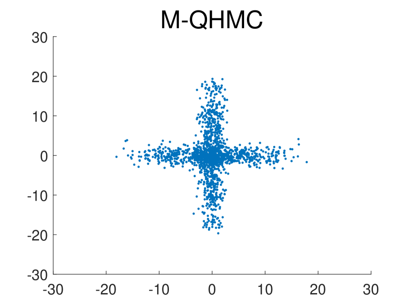
(f)

Figure 12: A two-dimensional Gaussian mixture example. (a) samples drawn from the ground truth distribution. (b)-(f) five methods used for sampling: HMC, randomized HMC, riemannian HMC, D-QHMC and M-QHMC. Only M-QHMC explores both Gaussians efficiently.

The results are shown in Fig. 12. Among the five methods, only M-QHMC can generate accurate sample distributions.

6.2 Application: Sparse Modeling via Bridge Regression

In data mining and machine learning, the following loss function is often minimized

$$L(\boldsymbol{\beta})=\frac{\mu}{2n}||\mathbf{y}-\mathbf{X}\boldsymbol{\beta}||_{F}^{2}+\lambda||\boldsymbol{\beta}||_{p}^{p}=L_{ls}(\mathbf{\beta})+L_{re}(\mathbf{\beta})$$ (48)

in order to learn a model. In Bayesian learning, this is equivalent to a linear model with Gaussian noise and $\ell_{p}$ prior. The likelihood function and prior distribution are $p({\cal D}|\mathbf{\beta})\propto{\rm exp}(-L_{ls}(\beta))$ and $p(\mathbf{\beta})\propto{\rm exp}(-L_{re}(\mathbf{\beta}))$ respectively, thus the posterior distribution is $p(\mathbf{\beta}|{\cal D})\propto p(\mathbf{\beta})p({\cal D}|\mathbf{\beta})\propto{\rm exp}(-L(\beta))$. In “bridge regression" (Polson et al., 2014; Armagan, 2009), the parameter $p$ is chosen in the range $(0,1)$ in order to select proper features and to enforce model sparsity. In a Bayesian stetting, this is equivalent to placing a prior ${\rm exp}(-\|\boldsymbol{\beta}\|_{p}^{p}/{\tau})$ over the unknown model paramters $\boldsymbol{\beta}$.

In this experiment, we consider the case $p=1/2$ and perform bridge regression using the Stanford diabetes dataset . This dataset includes $n=442$ people, 10 attributes (AGE, SEX, BMI, BP, S1-S6) and 1 health indicator (Y). The goal is to select as few attributes as possible but they still accurately predict the target Y. We split the dataset into a training set with 300 people and a testing set with 142 people. The hyper-parameters $\mu$ and $\lambda$ can be automatically determined if by further introducing some hyper-priors over $\lambda$ and $\mu$ (Polson et al., 2014; Armagan, 2009). However, the non-existence of analytical conjugate priors (Armagan, 2009) makes updates (Gibbs sampling) of $\mu$ and $\lambda$ only approximate, but not exact. For the sake of simplicity, we utilize a grid search method in the $(\lambda,\mu)$ plane with the testing MSE (mean-squared error) as a criteria to choose the hyper-parameters. We start from $\boldsymbol{\beta}=\mathbf{0}$ and use 1000 paths of gradient descent as a burn-in process. After that, we run another 1000 paths of HMC/QHMC and collect the samples. The results are shown in Table 2 for both HMC and QHMC. When the regularization $\lambda$ is small ($\lambda=0.1,1,10$), the difference between HMC and QHMC is insignificant; however, when large regularization is required for very sparse models (e.g. $\lambda=100$ or $1000$), QHMC can produce models with higher accuracy.

Table 2: Testing mean-squared error (MSE) for the bridge regression task

HMC/QHMC		$\mu$
		0.1	1	10	100
$\lambda$	0.1	4.20/5.14	0.68/0.69	0.29/0.29	0.25/0.25
	1	0.71/1.05	0.52/0.52	0.30/0.30	0.26/0.25
	10	0.51/0.51	0.51/0.46	0.51/0.49	0.31/0.28
	100	0.64/0.48	0.88/0.58	0.72/0.50	0.69/0.52
	1000	3.9/2.7	30.4/23.6	15.9/9.3	2.4/0.8

Table 3: CPU time and accuracy comparison of QHMC with some baseline methods.

	S-QHMC/D-QHMC	HMC	RMHMC	NUTS
CPU time(s)	3.9/4.1	3.8	9.8	98.3
test MSE	0.28/0.29	0.31	0.98	0.28

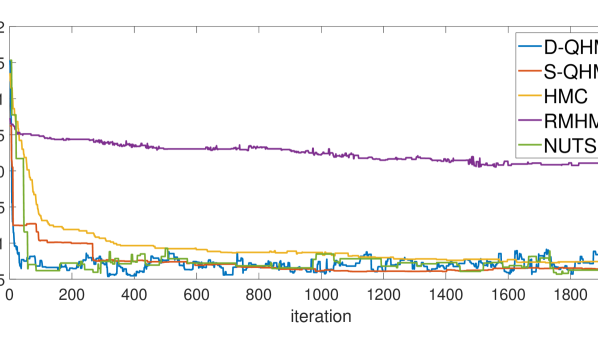
(a)

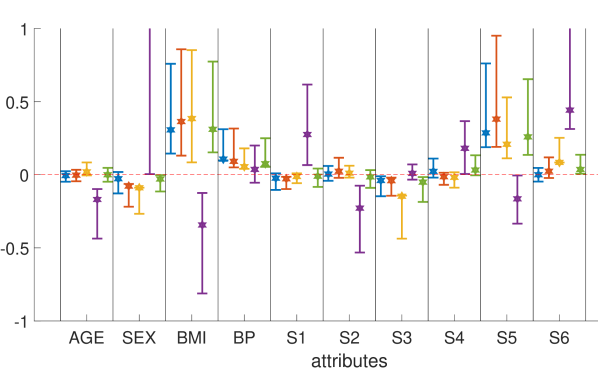
(b)

Figure 13: (a) The log testing error as a function of the iteration step. The number of steps required by burn-in process in QHMC ($\sim 500$ steps) is much smaller than that in HMC ($\sim 2000$ steps). (b) Distribution of all attributes in the diabetes dataset using QHMC, HMC, NUTS and RMHMC with $\mu=100$ and $\lambda=10$. QHMC is better at sampling sparser models than standard HMC (QHMC produces smaller variance in coefficients) and has smaller MSE on the testing data.

We consider the case with $\lambda=10$ and $\mu=100$, and compare S-QHMC and D-QHMC against the standard HMC, NUTS (Hoffman and Gelman, 2014) and RMHMC (Girolami and Calderhead, 2011). The resulting test MSE and CPU time are reported in Table 3. RMHMC is implemented with $(\mathbf{X}^{T}\mathbf{X})$ (with $\mathbf{X}$ being the data matrix) being the metric of the Riemannian manifold in (Girolami and Calderhead, 2011), and NUTS is implemented based on Alg. 2 in (Hoffman and Gelman, 2014). Although RMHMC is an adaptive HMC, it tends to degrade for spiky energy functions. Because the $\ell_{p}$ penalty is isotropic (i.e., the regularization coefficients for all attributes are the same), imposing an anisotropic metric renders the sampling performance even worse than HMC. NUTS can achieve comparable test MSE with QHMC, nontheless it consumes $25\times$ more CPU time than QHMC due to the expensive recursions of building balanced binary trees. Compared with HMC, QHMC has three advantages. Firstly, QHMC is more accurate as shown by the lower test MSE. Secondly, QHMC has a much shorter burn-in phase than HMC, as shown in Fig. 13 (a). This is expected because the possible small masses in QHMC can speed up the burn-in phase. Thirdly, QHMC can produce sparser models than HMC as expected. As shown in Fig. 13 (b), seven attributes have nearly zero mean (except BMI, S3 and S5). The samples from QHMC have smaller variance for these seven attributes, implying a more spiky posterior sample distribution of $\boldsymbol{\beta}$. Besides, D-QHMC achieves similar CPU time and test MSE with S-QHMC, but can produce sparser samples (see attributes SEX, S2 and S6 in Fig. 13 (b)).

6.3 Application: Image Denoising

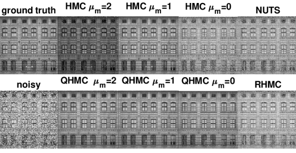
(a)

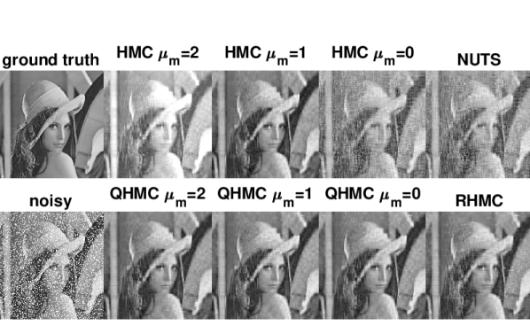
(b)

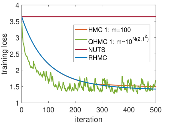
(c)

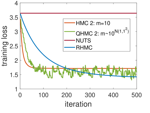
(d)

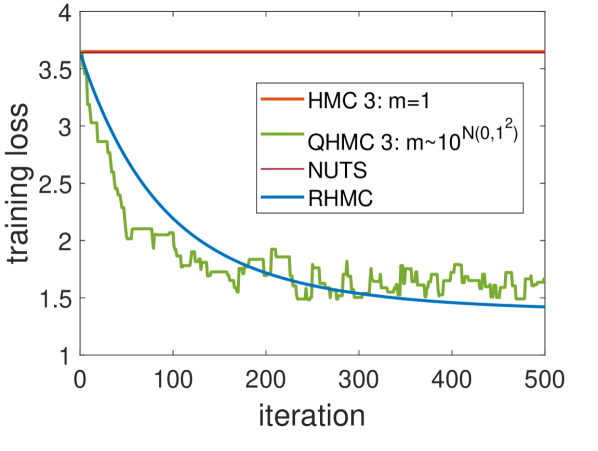
(e)

Figure 14: Image denoising example. Here we choose S-QHMC to implement QHMC. (a)(b) HMC can achieve good reconstruction only for the second parameters, while QHMC has good performance for all settings and its performance is much less sensitive to the choice of mass parameters. Also, Neither NUTS or RMHMC can achieve comparable results with QHMC. (c) For small step size (large mass), QHMC can speed up convergence in the large gradients phase; (d) For proper step size, HMC and QHMC show no significant difference. (e) For large step size (small mass), QHMC can still make progress in terms of decreasing the loss function, while HMC gets stuck at high loss.

In this experiment, we apply QHMC to solve an image denoising problem.

Specifically, we consider a two-dimensional gray-level image, but the extension to high-order tensors is available (Sobral et al., 2015). We employ the robust low-rank matrix factorization model (Candès et al., 2011) which models a corrupted image $\mathbf{Y}$ as the sum of a low-rank matrix $\mathbf{L}=\mathbf{A}\mathbf{B}$, a sparse matrix $\mathbf{S}$ describing outliers and some i.i.d. Gaussian noise. Standard robust PCA uses $\ell_{1}$-norm to enforce the sparsity of $\mathbf{S}$. Instead, we employ $\ell_{p}$ norm with $p=1/2$ because it is closer to the exact sparsity measurement $\ell_{0}$-norm. As a result, we can define the potential energy function as follows:

$$U(\mathbf{A},\mathbf{B},\mathbf{S})=L_{g}+L_{l}+L_{n}=\frac{1}{2}\mu||\mathbf{Y}-\mathbf{AB}-\mathbf{S}||_{F}^{2}+\frac{1}{2}\lambda_{1}(||\mathbf{A}||_{F}^{2}+||\mathbf{B}||_{F}^{2})+\lambda_{2}||\mathbf{S}||_{p}^{p}$$ (49)

In the Bayesian setting, ${\rm exp}(-L_{g})$ refers to the likelihood function; ${\rm exp}(-L_{l})$ refers to the prior density of the low rank part; ${\rm exp}(-L_{n})$ refers to the prior of the salt-and-pepper noise (which is sparse in nature). The gradient of the above loss function with respect to $\mathbf{A}$, $\mathbf{B}$ and $\mathbf{S}$ are:

$$\left\{\begin{aligned} \frac{\partial U}{\partial\mathbf{A}}&=\mu(\mathbf{AB}+\mathbf{S}-\mathbf{Y})\mathbf{B}^{T}+\lambda_{1}\mathbf{A}\\ \frac{\partial U}{\partial\mathbf{B}}&=\mu\mathbf{A}^{T}(\mathbf{AB}+\mathbf{S}-\mathbf{Y})+\lambda_{1}\mathbf{B}\\ \frac{\partial U}{\partial\mathbf{S}}&=\mu(\mathbf{AB}+\mathbf{S}-\mathbf{Y})+\lambda_{2}\frac{p_{0}}{\mathbf{S}^{1-p_{0}}+\epsilon_{0}}\mathrm{sign}(\mathbf{S}).\end{aligned}\right.$$ (50)

In the second term of the gradient with respect to $\mathbf{S}$, all operations are element-wise, and $\mathrm{sign}(x)$ is defined as

$$\mathrm{sign}(x)=\left\{\begin{aligned} 1,&\quad x\geq 0\\ -1,&\quad x<0.\end{aligned}\right.$$ (51)

The parameters are fine tuned and set as $\mu=100$, $\lambda_{1}=1$, $\lambda_{2}=10$, $p=1/2$ and the rank $r=20$. It is possible to automatically determine the rank by introducing some hyper-priors (e.g. (Zhao et al., 2015)), but here we focus on the sampling of a given model with a spiky loss function.

We use the proposed QHMC method (both D-QHMC and S-QHMC) to draw samples from the model, and we compare it with HMC, RMHMC (Girolami and Calderhead, 2011) and NUTS (Hoffman and Gelman, 2014). In all experiments we initialize the model with Singular Value Decomposition (SVD) of the corrupted image and run 300 iterations as burn-in and another 200 iterations to collect the sample images. In HMC and QHMC, we use three groups of parameter choices for the mass matrix. The metric of the Riemannian manifold (Girolami and Calderhead, 2011) in RMHMC is chosen as a diagonal matrix whose diagonal elements are the singular values of the corrupted image. The NUTS is implemented based on Alg. 2 in (Hoffman and Gelman, 2014).

We show the image denoising results and convergence behaviors of QHMC, HMC, NUTS and RMHMC in Fig. 14(a)–(e). We use the peak signal to noise ratio (PSNR) as the measure of denoising effects and report the results in Table 4. The standard HMC method is very sensitive to parameter choices, because it can only provide good results with the 2nd group of parameter setting. In contrast, our QHMC method shows good performance for all parameters choices. RMHMC achieves similar performance with HMC ($\mu_{m}=1$), only decreasing the training loss faster for larger iteration steps. However, RMHMC still fails to produce comparable denoising effects with QHMC. NUTS converges very slowly for this example because the “U-Turn" criteria is easily satisfied in the spiky regions. Consequently, the recursions of balanced binary tree terminate quickly in NUTS, leading to low mixing rates. The difference between D-QHMC and S-QHMC in this example is nearly negligible as shown in Table 4, and in Fig. 14 we only showed the results for S-QHMC.

Table 4: Image denoising example: PSNR for different algorithms

Algorithm	S-QHMC/D-QHMC with $m=10^{{\cal N}(\mu_{m},1)}$			NUTS
	$\mu_{m}=2$	$\mu_{m}=1$	$\mu_{m}=0$	(Hoffman and Gelman, 2014)
PSNR	23.72/23.80	23.98/23.94	23.96/24.06	17.01
Algorithm	HMC with $m=10^{\mu_{m}}$			RMHMC
	$\mu_{m}=2$	$\mu_{m}=1$	$\mu_{m}=0$	(Girolami and Calderhead, 2011)
PSNR	14.94	23.61	17.03	22.40

6.4 Application: Bayesian Neural Network Pruning

Finally we apply the stochastic gradient implementation of our QHMC method to the Bayesian pruning of neural networks. Neural networks (Neal, 2012; Schmidhuber, 2015) have achieved great success in wide engineering applications, but they are often over-parameterized. In order to reduce the memory and computational cost of deploying neural networks, pruning techniques (Karnin, 1990) have been developed to remove redundant model parameters (e.g. weight parameters with tiny absolute values).

In this experiment we consider training the following two-layer neural network

$$\mathbf{\hat{y}}=\mathrm{softmax}(\mathrm{relu}(\mathbf{W}_{2}\mathrm{relu}(\mathbf{W}_{1}\mathbf{x}+\mathbf{b}_{1})+\mathbf{b}_{2}))$$ (52)

to classify the MNIST dataset (LeCun and Cortes, 2010). Here “relu" means a ReLU activation function; $\mathbf{W}_{1}\in\mathbb{R}^{784\times 200}$ and $\mathbf{W}_{2}\in\mathbb{R}^{200\times 10}$ are the weight matrices for the 1st and 2nd fully connected layers; a softmax layer is used before the output layer. The log-likelihood of this neural network is a cross-entropy function. We introduce the $\ell_{p}(p=1/2)$ priors, ${\rm exp}(-\lambda||{\rm Vec}(\mathbf{W}_{1})||_{p}^{p})$ and ${\rm exp}(-\lambda||{\rm Vec}(\mathbf{W}_{2})||_{p}^{p})$ with $\lambda=0.0001$, for the weight matrices $\mathbf{W}_{1}$ and $\mathbf{W}_{2}$ to enforce their sparsity. The resulting potential energy function is thus

$$U(\mathbf{W_{1}},\mathbf{W_{2}},\mathbf{b_{1}},\mathbf{b_{2}})=\sum_{i=1}^{N}\sum_{j=1}^{c}-\mathbf{y}_{i,c}{\rm log}(\hat{\mathbf{y}}_{i,c})+\lambda||{\rm Vec(\mathbf{W_{1}})}||_{p}^{p}+\lambda(||{\rm Vec(\mathbf{W_{2}})}||_{p}^{p}$$ (53)

where $c$ is the number of classes (10 for MNIST), $\mathbf{y}$ is the ground truth label vector, and ${\rm Vec}$ is an operator that vectorizes the matrix. For simplicity we employ uniform prior distributions for $\mathbf{b_{1}}$ or $\mathbf{b_{2}}$. Due to the large training data set (with 60000 images), we use the stochastic gradient implementation with a batch size of 64 in the stochastic gradient Nosé-Hoover thermostat (SGNHT) (Ding et al., 2014) and in our proposed quantum stochastic gradient Nosé-Hoover thermostat (QSGNHT). In (Chen et al., 2014) it is shown that a naive implementation of stochastic gradient HMC can produce wrong steady distributions, therefore we utilize the thermostat method (Ding et al., 2014) to correct the steady distributions, and adopt the QSGNHT algorithm proposed in Section 5. Our proposed QSGNHT is slightly different from SGHMC (Chen et al., 2014) in the practical implementation. Firstly, we implement the MH step where a Hamiltonian is estimated based on a batch of samples, although no MH steps are used in (Chen et al., 2014) due to efficiency considerations. Secondly, we set a lower bound $m_{0}$ for $m$: if a sampled mass $m$ is smaller than $m_{0}$, then we set $m=m_{0}$. Both tricks help avoid very large model updates because $m$ can be arbitrarily close to 0 if there is no lower bound for $m$.

Table 5: Bayesian pruning results of a 2-layer neural network classifier for the MNIST dataset. Comp rate: compression rate; Test acc: test accuracy.

	SGNHT	SGHMC	SGLD	QSGNHT
	(Ding et al., 2014)	(Chen et al., 2014)	(Welling and Teh, 2011)	(proposed)
Comp rate	$47.6\pm 1.3$	$32.2\pm 1.5$	$30.8\pm 1.4$	54.2 $\pm$ 2.1
Test acc (%)	$94.4\pm 0.2$	$95.2\pm 0.2$	$93.2\pm 0.2$	96.6 $\pm$ 0.2

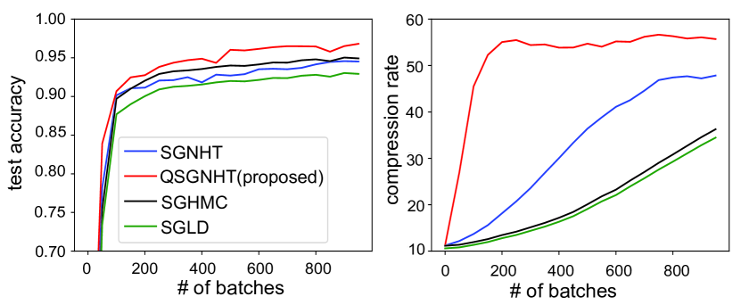
Figure 15: Bayesian pruning of a neural network with QSGNHT (proposed), SGNHT, SGHMC and SGLD. Left: testing accuracy; Right: compression rate.

We choose $m=10^{1}$ for SGNHT and $m\sim 10^{{\cal N}(1,0.5^{2})},m_{0}=1$ for QSGNHT, and run 1000 steps to collect random samples based on Hamiltonian simulations. We set a weight parameter to 0 if its absolute value is below $0.01$. The resulting compression rate is measured as:

$$\mathrm{Compression\ rate}=\frac{\mathrm{\#\ of\ all\ weight\ parameters}}{\mathrm{\#\ of\ paramters\ after\ pruning}}.$$ (54)

We plot the test accuracy estimated on 10000 test images and the compression rate as a function of the total number of training batches accessed in gradient evaluations, shown in Fig. 15. Our method is compared with SGNHT (Ding et al., 2014), SGHMC (Chen et al., 2014) and SGLD (Welling and Teh, 2011). SGHMC is implemented in the framework of SGNHT with the paramter setting $\xi=1$ and $m_{\mu}=\infty$. SGLD is implemented by excluding the momentum in SGHMC and directly updating the network with gradients. We consider the first 800 batches as the burn-in phase and use the simulation samples in last 200 batches. The test accuracy and compression rate for the neural network samples are reported in Table 5. For test accuracy, our proposed QSGNHT achieves $2\%$ accuracy improvement compared with SGNHT (Ding et al., 2014). SGHMC and SGLD also underperform QSGNHT in terms of test accuracy. Regarding the compression rate, the third-order Langevin dynamics (QSGNHT and SGNHT) outperform the second-order Langevin dynamics (SGHMC) and first-order (SGLD) Langevin dynamics. Besides, the proposed QSGHNT achieves 14% more compression rate than SGNHT.

7 Conclusions

Leveraging the energy-time uncertainty relation in quantum mechanics, we have proposed a quantum-inspired Hamiltonian Monte Carlo method (QHMC) for Bayesian sampling. Different from the standard HMC, our method sets the particle mass matrix as a random variable associated with a probability distribution. We have proved the convergence of its steady state (both in space and in time sequence) to the true posterior density, and have theoretically justified its advantage over standard HMC in sampling from spiky distributions and multimodal distributions. In order to improve the efficiency of QHMC in massive-data scenarios, we have proposed a stochastic-gradient implementation with Nosé-Hoover thermostat terms and proved its theoretical properties. We have discussed S-QHMC, D-QHMC and M-QHMC as three special yet useful parametrizations of QHMC and have demonstrated their advantages over HMC and its variants by several synthetic examples. Finally, we have applied our methods to solve several classical Bayesian learning problems including sparse regression, image denoising and neural network pruning. Our methods have outperformed HMC, NUTS, RMHMC and several stochastic-gradient implementations on these realistic examples. In the future, we plan to develop a deeper theoretical understanding of QHMC and more robust and efficient implementation for large-scale learning problems.

Acknowledgments

This work was partly supported by NSF CCF-1817037 and NSF CAREER Award No. 1846476. The authors would like to thank Kaiqi Zhang, Cole Hawkins and Dr. Chunfeng Cui for their valuable technical suggestions.

References

- Armagan (2009) Artin Armagan. Variational bridge regression. In Artificial Intelligence and Statistics, pages 17–24, 2009.
- Bakry et al. (2008) Dominique Bakry, Patrick Cattiaux, and Arnaud Guillin. Rate of convergence for ergodic continuous markov processes: Lyapunov versus poincaré. Journal of Functional Analysis, 254(3):727–759, 2008.
- Beskos et al. (2011) A. Beskos, F.J. Pinski, J.M. Sanz-Serna, and A.M. Stuart. Hybrid monte carlo on hilbert spaces. Stochastic Processes and their Applications, 121(10):2201 – 2230, 2011. ISSN 0304-4149. doi: https://doi.org/10.1016/j.spa.2011.06.003. URL http://www.sciencedirect.com/science/article/pii/S0304414911001396.
- Borovkov (1998) Aleksandr Alekseevich Borovkov. Ergodicity and Stability of Stochastic Processes. J. Wiley, 1998.
- Bou-Rabee and Sanz-Serna (2017) Nawaf Bou-Rabee and Jesús María Sanz-Serna. Randomized hamiltonian monte carlo. The Annals of Applied Probability, 27(4):2159–2194, Aug 2017. ISSN 1050-5164. doi: 10.1214/16-aap1255. URL http://dx.doi.org/10.1214/16-AAP1255.
- Candès et al. (2011) Emmanuel J Candès, Xiaodong Li, Yi Ma, and John Wright. Robust principal component analysis? Journal of the ACM (JACM), 58(3):11, 2011.
- Chaari et al. (2016) Lotfi Chaari, Jean-Yves Tourneret, Caroline Chaux, and Hadj Batatia. A Hamiltonian Monte Carlo Method for Non-Smooth Energy Sampling. IEEE Transactions on Signal Processing, 64(21):5585–5594, 2016.
- Chaari et al. (2017) Lotfi Chaari, Jean-Yves Tourneret, and Hadj Batatia. A General Non-Smooth Hamiltonian Monte Carlo Scheme Using Bayesian Proximity Operator Calculation. In European Signal Processing Conference (EUSIPCO), pages 1220–1224, 2017.
- Chen et al. (2014) Tianqi Chen, Emily Fox, and Carlos Guestrin. Stochastic gradient Hamiltonian Monte Carlo. In International conference on machine learning, pages 1683–1691, 2014.
- Ding et al. (2014) Nan Ding, Youhan Fang, Ryan Babbush, Changyou Chen, Robert D Skeel, and Hartmut Neven. Bayesian sampling using stochastic gradient thermostats. In Advances in neural information processing systems, pages 3203–3211, 2014.
- Donoho et al. (2006) David L Donoho et al. Compressed sensing. IEEE Transactions on information theory, 52(4):1289–1306, 2006.
- Duane et al. (1987) S. Duane, A. D. Kennedy, B. J. Pendleton, and D. Roweth. Hybrid Monte Carlo. Phys. Lett., B195:216–222, 1987. doi: 10.1016/0370-2693(87)91197-X.
- Eckart (1953) Carl Eckart. Relation between time averages and ensemble averages in the statistical dynamics of continuous media. Phys. Rev., 91:784–790, Aug 1953.
- Eldar and Kutyniok (2012) Yonina C Eldar and Gitta Kutyniok. Compressed Sensing: Theory and Applications. Cambridge university press, 2012.