Proximal Newton Methods for X-Ray Imaging with Non-Smooth Regularization
Abstract
Non-smooth regularization is widely used in image reconstruction to eliminate the noise while preserving subtle image structures. In this work, we investigate the use of proximal Newton (PN) method to solve an optimization problem with a smooth data-fidelity term and total variation (TV) regularization arising from image reconstruction applications. Specifically, we consider a nonlinear Poisson-modeled single-energy X-ray computed tomography reconstruction problem with the data-fidelity term given by the I-divergence. The PN algorithm is compared to state-of-the-art first-order proximal algorithms, such as the well-established fast iterative shrinkage and thresholding algorithm (FISTA), both in terms of number of iterations and time to solutions. We discuss the key factors that influence the performance of PN, including the strength of regularization, the stopping criterion for both sub-problem and main-problem, and the use of exact or approximated Hessian operators.
Introduction
Structures in medical images are critical, providing information inside the human body for diagnosis and development of treatment plans. However, an improper regularization term may eliminate subtle structures during image reconstruction [1, 2]. Non-smooth regularization terms, such as norm or total variation (TV) [3, 4], are widely used in image reconstruction to enforce sparsity (either in the image, wavelet, or gradient domain) while reducing noise. For these methods to be useful in clinical diagnosis and research, the images should be reconstructed within a clinically acceptable time.
The use of TV regularization is often advocated in imaging applications because of its ability to preserve sharp edges in the reconstructed image; however, the non-smoothness of the TV functional poses a substantial challenge to the efficient solution of the corresponding optimization problem.
Proximal gradient algorithms (such as FISTA) [5] represent the state-of-art to solve image reconstruction problems with non-smooth regularization terms like TV. However, these methods still require hundreds of iterations to converge and each iteration requires to evaluate the smooth data fidelity term and its gradient. This can be extremely time-consuming for problems, such as transmission tomography, where the imaging operator is expensive to compute [6, 7].
Our goal is to investigate more efficient solution algorithms for this class of problems that exploit curvature information (the Hessian of the smooth data-fidelity term) to achieve faster convergence than classical proximal gradient methods. Specifically, we numerically show that, for our target application, Proximal Newton method can outperform state-of-the-art proximal gradient methods, such as FISTA, and we also discuss key factors that influence the performance of the algorithm.
Second-order proximal methods, and proximal Newton in particular, have mostly been explored in the fields of bioinformatics [8], signal processing [9], and statistical learning [10, 11]. To the best of our knowledge, this is the first time that proximal Newton methods are applied to an image reconstruction problem with TV penalty term. Our results suggest that for our target problem, and possibly for many other problems in which evaluations of the smooth data fidelity term are computationally expensive, PN is faster than state-of-the-art proximal first order methods, such as FISTA.
Method
We consider the problem of minimizing a composite function
| (1) |
where is the smooth data fidelity term and is the non-smooth penalty term.
The proximal Newton method minimizes the composite function by successively constructing and minimizing a surrogate function [12, 13]. At each iteration , the PN algorithm performs three steps.
1. Surrogate function construction.
In the first step, the PN method computes the surrogate function by approximating the smooth data fidelity term with its second order Taylor approximation centered at the current iterate , that is
| (2) |
where and are the gradient and Hessian of function at .
2. Surrogate minimization.
In the second step, the PN method computes a search direction by minimizing , that is
| (3) |
This subproblem does not usually admit a closed-form solution and need to solved iteratively, possibly using a first-order proximal algorithm such as FISTA. Note that the solution of this subproblem does not require any evaluations of the (computationally expensive) data fidelity term or of its gradient.
3. Solution update.
In the third and last step, the PN method updates the iterate as
| (4) |
where the step size is calculated by back-tracking line search to ensure the sufficient descent condition
| (5) |
for some .
The pseudo-code for PN algorithm is shown in Algorithm 1.
It is worth to notice that the performance and practical usefulness of the PN method strongly depends on the availability of computational efficient solver for the surrogate minimization problem in (3). To this aim, we consider the two complementary approaches proposed in [13].
First, one can reduce the computational cost of evaluating the surrogate function and its proximal gradient by replacing the true Hessian matrix with a cheaper-to-apply Quasi-Newton approximation of , such as that given by the (limited-memory) Broyden-Fletcher-Goldfarb-Shanno (BFGS) algorithm [14].
Second, one can solve subproblem (3) inexactly by an using early stopping criterion, such as a fixed maximum iterations or an adaptive stopping condition, to get an inexact solution with much less inner iterations. Simply put, one need not solve subproblem (3) accurately when the surrogate function in (2) is an inaccurate approximation of the objective function . Rather, to preserve the fast convergence rate of PN methods, one should solve (3) accurately only when is near the optimal solution or is an accurate approximation to . Following [13], we then generalize the adaptive stopping condition originally introduced by Eisenstat and Walker in 1996 [15] for smooth problems as follows:
| (6) |
where is the outer iteration index, and is the proximal mapping of the non-smooth term, and is the gradient of the approximated smooth term evaluated at . Here, is a forcing term that satisfies
| (7) |
Target application
In the numerical results presented in the next section, we consider the minimization of a composite function arising in single-energy X-ray computed tomography (CT) reconstruction problems [7].
Here, denotes the sought-after linear attenuation coefficient (image), the data fidelity stems from a Poisson negative log-likelihood function, and the regularization term is an isotropic TV function [3]
| (8) |
where denote a 2-D index in the image domain, and controls the strength of regularization. The proximal mapping of total variation is solved by fast gradient projection [16], which iteratively projects and updates the image in its gradient domain.
In what follow we provide a derivation for the expression of the statistically inspired data fidelity term and of its gradient and Hessian. The CT reconstruction problem is modeled as an estimation of means of independent Poisson random variables. The survival probability of a photon that is transmitted through the target follows the Poisson distribution, and the mean of the photon counts is given by the Beer’s law:
| (9) |
where denotes the index in image (pixels) and measurement (ray) domain, respectively, is the attenuation coefficient to be estimated, denotes mean number of photons, and represents the length of the path of ray in pixel , whose matrix form is written as .
Maximizing the Poisson likelihood is equivalent to minimizing I-divergence function
| (10) |
where is the measured transmission data obtained from the scanner. Finally, the gradient of is given by
| (11) |
and the second-order derivative of reads
| (12) |
where is a square diagonal matrix with entries .
The matrix is formally a dense operator of size number of pixels by number of pixels and shall not be computed explicitly. For example, consider a two-dimensional reconstruction problem of a image, then would be a dense matrix, those storage would require more than gigabytes memory using double precision. This memory requirement would then increase of a factor 16 when doubling the image resolution. To put things in perspective, a 3-dimensional CT reconstruction problem of practical relevance commonly involves images with resolution of pixels, thus requiring about 21 petabytes memory to store the Hessian matrix, which is impossible for the nowadays computational devices.
On the other hand, the PN algorithm does not require to explicitly access to the matrix , but only the ability to compute the action of in a direction . This action can be computed matrix-free at the cost of performing one set of forward and back-projection steps as summarized in Algorithm 2. It is worth noticing that if the forward and back-projection steps are also computed matrix-free, then the only memory requirement is that of storing two vectors on the same dimension of the data, namely the scaling vector and the intermediate vector .
Result
For all three sets of experiments presented below, we consider a CT system with 90 equispaced projection spanning a 180-degree angle and 90 rays per projection. The Shepp-Logan phantom generated by MATLAB built-in function is used as ground-truth. The noiseless measured data is obtained by exponentiation of the forward-projection of the ground truth,
| (13) |
while the noisy data is a realization from a Poisson random vector whose mean is equal to the noiseless data
| (14) |
In each experiment, the strength of regularization is chosen by the generalized L-curve criterion. Unless otherwise indicated, default reconstruction parameters and PN algorithm settings are shown in the table below.
| Image Size | pixels |
|---|---|
| Sinogram Size | pixels |
| Diameter of FOV | 512 mm |
| Hessian Computation | Exact |
| Initial Guess | Zeros |
| PN Stopping Criterion | |
| Max iter: 500 | |
| Subproblem Stopping Criterion | |
| Max iter: 500 | |
| Adaptive Stopping Condition |
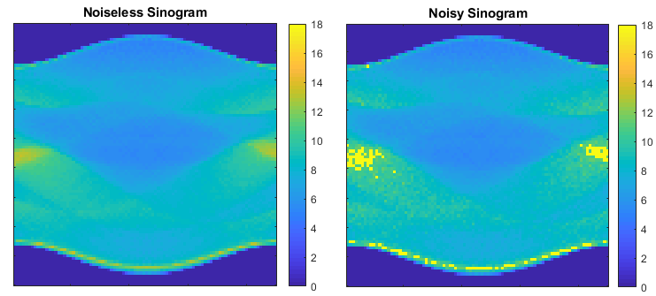
Figure 1 shows the negative log-scaled simulated transmission data with and without noise. It is worth noticing that we have clipped the range of values in the log-scaled sinogram for visualization purposes. Extremely bright-yellow values in the noisy sinogram correspond to detectors that fail to receive any photon.
For the computation below, we use a modified version of the PNOPT code [13] and TFOCS package [17] to solve the optimization problem using PN and FISTA, Airtools [18] to compute forward projection operator , and TV proximal function in UNLocBoX [19]. The forward projection operator was precomputed before solving the optimization problem and stored in a compressed sparse column (CSC) format to allow for fast application of the forward and back-projection steps within MATLAB.
Finally, the computer utilized for time analysis has a 20-threaded Intel Xeon E5 2630-v4 and 128 Gigabytes memory. No GPU computation is involved.
Efficiency comparison between PN and FISTA
The convergence rate of proximal Newton is compared to FISTA for an image size of pixels. Due to the higher convergence rate of second-order methods, PN greatly outperforms FISTA algorithm with respect to the number of outer iterations, as shown in Figure 2. PN takes approximately 20 iterations to achieve the minimum objective value, while FISTA takes more than 2,000 iterations. However, each PN outer iteration is more expensive that one FISTA iteration, since it requires solving subproblem (3) iteratively. In total, the cumulative number of PN inner iterations is about five time larger than the number of FISTA iterations.
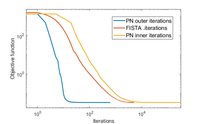
It is worth to notice that PN inner iterations are performed using the surrogate function in (2), and therefore are computationally less expensive then FISTA iterations. For this reason, Figure 3 compares the two algorithms in terms of computational time. Overall, PN achieves a 3 speedup in terms of time-to-solution compared to FISTA.
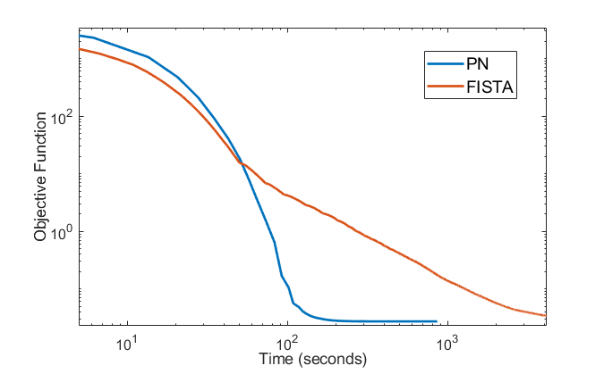
Comparing Figure 2 and Figure 3, we can argue that the computational cost of each inner iteration in the PN method is extremely less than the computational cost of each iteration in FISTA. In fact, PN only computes gradient and Hessian of the data-fidelity term in the outer iteration, while FISTA computes the gradient in every iteration. Thus, for problems in which evaluations of the smooth data fidelity term are computationally expensive, PN is more efficient.
Scalability of PN with respect to image resolution
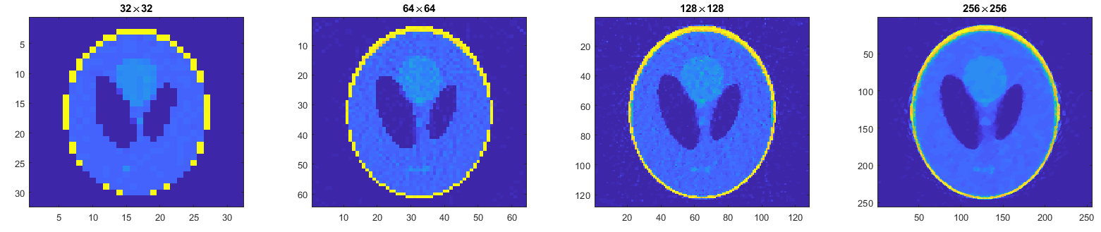
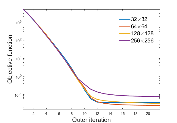
Figure 4 shows the reconstructed solution of the CT problem using the PN algorithm for different image resolutions. The image size ranges from to pixels with increases by a factor of , corresponding to the pixel size ranging from to , respectively. Also, the strength of regularization is increased by a factor of to match the image resolution.
The number of iterations required to converge is 14, 18, 19 and 20, respectively, as shown in Figure 5. This indicates that PN algorithm has almost perfect scalability with respect to problem size, similar to that of the classical Newton method for smooth problems.
Effect of Hessian computation
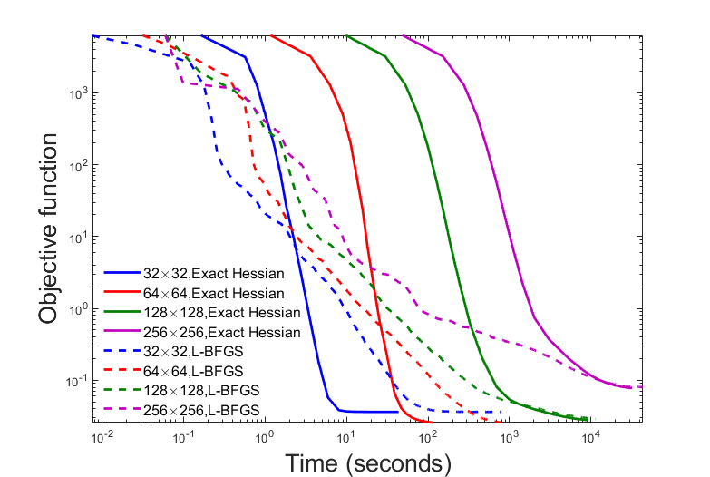
The BFGS algorithm approximates the Hessian matrix and its inverse from differences in the gradient and increments in the solution between iterates, and stores such approximation as a dense matrix. As previously discussed, storing the Hessian (or its approximation) as a dense matrix is unfeasible for medium to large scale problems, because of storage requirements. To address this issue, limited memory-BFGS computes the approximated action of the Hessian and its inverse using a limited number of updating vectors, thus drastically reducing storage requirements. Here, we compare the convergence of the PN algorithm using the exact Hessian and its L-BFGS approximation. In all experiments, we limit the maximum number of L-BFGS update vectors to 50. Results are shown in Figure 6.
For relatively small problem sizes (), the L-BFGS approximations achieves better performance in the early iterations but exact Hessian quickly catches up and allows to reach the target accuracy faster in terms of time-to-solution. As the problem dimension increases, L-BFGS approximation becomes more competitive due to the increased computational cost of evaluating the exact Hessian action. As shown in the figure, PN with L-BFGS approximation can outperform PN with exact Hessian with respect to time-to-solution for large-scale images and practical accuracy requirements.
To sum up, if a coarse accuracy is needed, L-BFGS outperforms exact Hessian for large scale problems, however as one increases the accuracy requirements using the exact Hessian will eventually pay off. Another advantage of using the exact Hessian operator is that—when memory is the limiting factor—evaluating the action of the exact Hessian on a vector using Algorithm 2 only requires to store two temporary vectors with the same dimension of the data, while L-BFGS requires storing several updating vectors of the same dimension of the image.
Conclusion
In this paper, we demonstrated an application of proximal Newton (PN) method to X-Ray tomography reconstruction problems with total variation regularization and synthetic sinogram data. At each iteration, the PN method minimizes a surrogate objective function where the smooth and computationally expensive data fidelity term is approximated by its second-order Taylor’s expansion.
Numerical results indicates that the PN algorithm can outperform state-of-the-art first-order proximal algorithms (such as FISTA) not only in terms of number of gradient evaluations but also in terms of time-to-solution for the application considered here. In addition, we numerically verified that the PN algorithm converges in a number of iterations that is almost independent of problem size, thus enjoying scalability properties similar to that of the classical Newton method for smooth problems.
Finally, we compared the effect of different Hessian approximations on PN performance. In particular, the L-BFGS approximation of the Hessian drastically reduces the computational cost of minimizing the PN surrogate objective functions, thus allowing for faster (in terms of time) progress in the early iterations of the algorithm. This speed-up in the initial phase of the algorithm becomes more and more evident as the resolution is increased. However, when the optimization problem needs be solved with high accuracy, using the exact Hessian will eventually outperforms the L-BFGS approximation due the its higher rate of convergence.
References
- [1] P. Charbonnier CNRS-UNSA, L. Blanc-Feraud, G. Aubert, and M. Barlaud. Deterministic edge-preserving regularization in computed imaging. IEEE Transactions on Image Processing, 6(2):298–311, Feb 1997.
- [2] Hao Zhang et al. Regularization strategies in statistical image reconstruction of low-dose x-ray CT: A review. Medical physics, 45(10):886–907, 2018.
- [3] Leonid I. Rudin, Stanley Osher, and Emad Fatemi. Nonlinear total variation based noise removal algorithms. Physica D: Nonlinear Phenomena, 60(1):259 – 268, 1992.
- [4] David Dobson and Otmar Scherzer. Analysis of regularized total variation penalty methods for denoising. Inverse Problems, 12(5):601–617, oct 1996.
- [5] Amir Beck and Marc Teboulle. A fast iterative shrinkage-thresholding algorithm for linear inverse problems. SIAM J. Imaging Sci., 2(1):183–202, 2009.
- [6] Kenneth Lange and Richard Carson. EM reconstruction algorithms for emission and transmission tomography. Journal of computer assisted tomography, 8:306–316, 05 1984.
- [7] J. A. O’Sullivan and J. Benac. Alternating minimization algorithms for transmission tomography. IEEE Transactions on Medical Imaging, 26(3):283–297, March 2007.
- [8] W. Geng K. Zhang and S. Zhang. Network-based logistic regression integration method for biomarker identification. BMC Syst. Biol., 12(135), 2018.
- [9] Niccolò Antonello, Lorenzo Stella, Panagiotis Patrinos, and Toon Waterschoot. Proximal gradient algorithms: Applications in signal processing. 03 2018.
- [10] Xuanqing Liu, Cho-Jui Hsieh, Jason Lee, and Yuekai Sun. An inexact subsampled proximal Newton-type method for large-scale machine learning. 08 2017.
- [11] Yuchen Zhang and Xiao Lin. DiSCO: Distributed optimization for self-concordant empirical loss. In Francis Bach and David Blei, editors, Proceedings of the 32nd International Conference on Machine Learning, volume 37 of Proceedings of Machine Learning Research, pages 362–370, Lille, France, 07–09 Jul 2015. PMLR.
- [12] S. Gunter J. Yu, S.V.N. Vishwanathan and N.N. Schraudolph. A quasi-Newton approach to nonsmooth convex optimization problems in machine learning. J. Mach. Learn. Res., 11:1145–1200, 2010.
- [13] Yuekai Sun Jason D. Lee and Michael A. Saunders. Proximal Newton-type methods for minimizing composite functions. SIAM J. Optim., 24(3):1420–1443, 2014.
- [14] Jorge Nocedal. Updating quasi-Newton matrices with limited storage. Mathematics of Computation, 35(151):773–782, 1980.
- [15] Stanley C. Eisenstat and Homer F. Walker. Choosing the forcing terms in an inexact Newton method. SIAM J. Sci. Comput., 17(1):16–32, 1996.
- [16] Amir Beck and Marc Teboulle. Fast gradient-based algorithms for constrained total variation image denoising and deblurring problems. IEEE Transactions on Image Processing, 18(11):2419–2434, Nov 2009.
- [17] E.J. Cand‘es S.R. Becker and M.C. Grant. Templates for convex cone problems with applications to sparse signal recovery. Math. Prog. Comp., 3(3):165–218, 2011.
- [18] Per Christian Hansen and Maria Saxild-Hansen. AIR tools — a MATLAB package of algebraic iterative reconstruction methods. Journal of Computational and Applied Mathematics, 236(8):2167 – 2178, 2012. Inverse Problems: Computation and Applications.
- [19] Nathanael Perraudin, David I. Shuman, Gilles Puy, and Pierre Vandergheynst. UNLocBoX A matlab convex optimization toolbox using proximal splitting methods. CoRR, abs/1402.0779, 2014.
Author Biography
Tao Ge received his BS in electrical engineering from Harbin Engineering University (2016) and his master in electrical engineering from Washington University in St. Louis (2018). Since then he has been a PhD candidate in electrical engineering of Washington University in St. Louis. His work has focused on CT reconstruction problems.
Umberto Villa received his BS and MS in Mathematical Engineering from Politecnico of Milano (Milan, Italy, 2005 & 2007) and his Ph.D. in Mathematics from Emory University (Atlanta, US, 2012). He joined the Electrical & Systems Engineering Department of Washington University in St. Louis in 2018. His work has focused on the computational and mathematical aspects of large-scale inverse problems, medical imaging, uncertainty quantification, optimal experimental design. He is a member of IEEE and SIAM.
Ulugbek S. Kamilov obtained his BSc and MSc in Communication Systems, and PhD in Electrical Engineering from EPFL, Switzerland, in 2008, 2011, and 2015, respectively. Since 2017, he is an Assistant Professor and Director of Computational Imaging Group (CIG) at Washington University in St. Louis. His research area is computational imaging, large-scale optimization, and machine learning with applications to optical microscopy, magnetic resonance and tomographic imaging. In 2017, he received the IEEE Signal Processing Society’s Best Paper Award. He is currently a member of IEEE Technical Committee on Computational Imaging and Associate Editor for the IEEE Transactions on Computational Imaging.
Joseph O’Sullivan joined the faculty in the Department of Electrical Engineering at Washington University in St. Louis (WashU) in 1987. He was the Director of the Electronic Systems and Signals Research Laboratory (ESSRL) from 1998 to 2007. Today, Professor O’Sullivan directs the Imaging Science and Engineering certificate program.