Formation of SMBH seeds in Population III star clusters through collisions : the importance of mass loss

Abstract

Runaway collisions in dense clusters may lead to the formation of supermassive black hole (SMBH) seeds, and this process can be further enhanced by accretion, as recent models of SMBH seed formation in Population III star clusters have shown. This may explain the presence of supermassive black holes already at high redshift, $z>6$. However, in this context, mass loss during collisions was not considered and could play an important role for the formation of the SMBH seed. Here, we study the effect of mass loss, due to collisions of protostars, in the formation and evolution of a massive object in a dense primordial cluster. We consider both constant mass loss fractions as well as analytic models based on the stellar structure of the collision components. Our calculations indicate that mass loss can significantly affect the final mass of the possible SMBH seed. Considering a constant mass loss of 5% for every collision, we can lose between 60-80% of the total mass that is obtained if mass loss were not considered. Using instead analytical prescriptions for mass loss, the mass of the final object is reduced by 15-40%, depending on the accretion model for the cluster we study. Altogether, we obtain masses of the order of $10^{4}M_{\odot}$, which are still massive enough to be SMBH seeds.

1 Introduction

A great number of supermassive black holes (SMBH) has already been detected at redshifts higher than 6 ($z=7.085$ in Mortlock et al. 2011, $z=7.54$ in Bañados et al. 2018), and the number is still continuously increasing. These high redshifts roughly correspond to the first billion years of evolution of the Universe. A significant challenge to our cosmological model is explaining the existence of such massive objects at early times; if we consider the Eddington accretion rate, which is the maximum rate at which a black hole can accrete gas in spherical symmetry, initial seed masses of order $10^{4}M_{\odot}$ are required in order to reach final masses of $10^{9}M_{\odot}$, when realistic spin parameters and accretion disk models are taken into account (Shapiro, 2005). The only solutions are very massive seeds or extended periods of super-Eddington accretion, which can persist in non-spherically symmetric circumstances where the Eddington rate can be breached, or possible combinations between the two in the early stages of the massive black hole evolution (Mayer et al., 2013).

The three main pathways for the formation of supermassive black holes are: stellar remnants in the context of massive Population III (in short Pop. III) stars, the collapse of a protogalactic gas cloud into a massive black hole or a massive star, that later collapses into a black hole, and seed black holes forming in dense stellar clusters via dynamical processes (Rees, 1984; Woods et al., 2018). One of the most promising explanations for massive seeds is the direct collapse model, as it can potentially produce the most massive seeds. In order to form massive black holes in this way, numerical simulations have shown that cooling needs to be suppressed, which can be achieved when a strong radiation background photodissociates the molecular hydrogen, therefore preventing strong fragmentation of the gas cloud (Bromm & Loeb, 2003; Wise et al., 2008; Latif et al., 2013).

The strength of the radiation background required to keep the gas atomic is parametrized via $J_{21}$, which describes the strength of the radiation background at 13.6 eV. A value of $J_{21}=1$ corresponds to a radiative background of $10^{-21}$erg s^-1 cm^-1 Hz^-1 per steradian. First investigations using numerical simulations suggested a critical value of $J_{21}\sim$ 100 to prevent the formation of molecular hydrogen (Shang et al., 2010), later investigations which considered updated chemical networks and more realistic models for the radiation background (see e.g. Sugimura et al., 2014; Agarwal & Khochfar, 2014) have given much larger critical values, of the order $10^{5}$ when applied in cosmological simulations (Latif et al., 2014, 2015). One of the biggest problems for the direct collapse scenario is the need of a large value of $J_{21}$ (Dijkstra et al., 2014).

Furthermore, metals and dust grains can also be the cause of fragmentation events. For metal line cooling, a metallicity of $10^{-3}$ Z_⊙ can already trigger fragmentation within cosmological simulations (Bovino et al., 2014), and if dust cooling is considered, the metallicities required are considerably lower, of the order of $10^{-5}$ Z_⊙ (Schneider et al., 2006; Dopcke et al., 2013; Bovino et al., 2016). The need of both having very strong radiation backgrounds, while keeping the gas metal free, leads to a strong need of fine-tuning, which at best can be satisfied under very rare conditions (eg, Agarwal et al., 2017). Recently, Suazo et al. (2019) studied the formation of SMBH seeds in this context, forming a single massive object of $\sim 10^{5}M_{\odot}$ when the UV background of $J_{21}$ is set to 10000, while when considering a UV background of $J_{21}=10$, there is fragmentation and the formation of various less massive seeds. These fragments had masses of $10^{3}-10^{4}M_{\odot}$, and even though less massive, they were still prone to merge into a more massive object.

The alternative pathway of early black hole formation in stellar clusters via dynamical processes has been studied to a smaller extent. Devecchi & Volonteri (2009) and Devecchi et al. (2012) developed analytical models which predict black hole masses of $100-1000M_{\odot}$ forming in the first stellar clusters. Katz et al. (2015) modeled the formation of a dense stellar cluster in a cosmological simulation, and showed the subsequent formation of a $\sim 1000M_{\odot}$ black hole via $N$-body simulations. Likewise, Sakurai et al. (2017) combined cosmological and $N$-body simulations which led to the formation of black holes in the first stellar clusters with $400-1900$ $M_{\odot}$. Reinoso et al. (2018) studied collisions in massive Pop. III clusters, showing there could be resulting black hole masses of up to $600M_{\odot}$.

Boekholt et al. (2018) were the first to explore the formation of massive black hole seeds from a dense stellar cluster, taking into account the interaction between gas-dynamical and stellar-dynamical processes, considering also the accretion of the protostars and consequently enhanced radii. Since the initially low mass Pop. III protostars would gain mass by accreting from the gas reservoir, and as the accretion rate might vary with cluster environment and cluster evolution, they defined 6 different accretion models, in which accretion depends on the gas availability and position of the protostar. The models are further described in Section 2 and summarized in table 1. They concluded that accretion-induced collisions in dense Pop. III protostellar systems, in the presence of a sufficiently large gas reservoir, are a viable mechanism for explaining the formation of the first massive black hole seeds. Stellar collisions in primordial star clusters can give rise to the formation of massive objects of $10^{4}-10^{5}M_{\odot}$ for all the models considered.

This investigation warranted follow up studies, to improve on the realism of the implementation and to include additional physics previously not considered. One important aspect not taken into account was the mass that might get lost whenever two protostars collide, which is the main focus of the study here.

Mass loss in collisions of main-sequence stars has been already explored to a considerable extent, for example, Dale & Davies (2006) found that in encounters that involve a massive main-sequence star and a low mass one, the mass loss is between 2-4%. Gaburov et al. (2008) studied mixing in massive stellar mergers, and the highest mass loss they obtained was 8.9%. Glebbeek & Pols (2008) modelled central collisions between low mass stars, obtaining mass losses of a few percent.

We present here an investigation which explores the effect of mass loss during collisions, on the formation of massive black hole seeds from a dense stellar cluster. The numerical methods used are described in Section 2, including our setup and the mass loss parametrizations, and the main results are presented in Section 3. We summarize our work and address the main conclusions in Section 4.

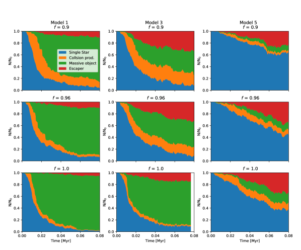
Figure 1: Fraction of stars over time corresponding to four categories: escapers (red); stars that have collided with and are part of the most massive star in the system (green, ‘Massive object’); stars that are part of other collision products (orange, ‘Collision prod.’); and single stars (blue), for different models, and different values for the fraction of mass conserved after a collision $f$. The general trend for the models is that the fraction of stars being part of the most massive object decreases when $f$ decreases.

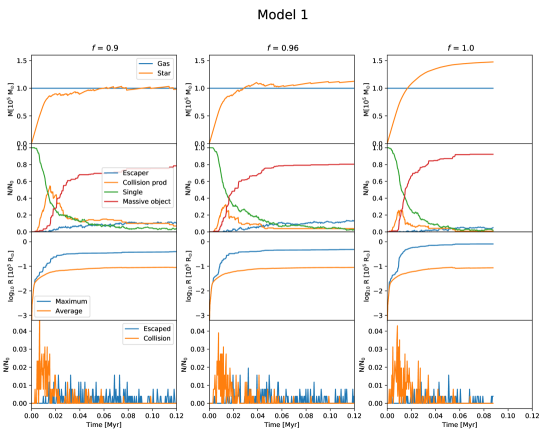
Figure 2: Correlation of the time evolution of the collision and escape rate (bottom panel) with: total star and gas mass (top panel), fraction of stars belonging to the same four categories as in Fig. 1 (second panel), and maximum stellar radius and average stellar radius of the remaining stars (third panel), for three different and representative values of the retained mass fraction $f$.

Figure 3: Same as Fig. 2 for model 3.

Figure 4: Same as Fig. 2 for model 5.

2 Numerical Methods

In order to model our astrophysical system, which consists of Pop. III protostars embedded in their natal gas cloud, we consider a variety of physical processes that play a role. Besides the gravitational $N$-body dynamics of the cluster, we model the gravitational coupling between the gas and the stars, include gas accretion which leads to stars growing in mass and size, and also handle collisions between stellar components of the system.

We use the Astrophysical MUlti-purpose Software Environment (AMUSE, Portegies Zwart & McMillan, 2018; Portegies Zwart et al., 2009; Portegies Zwart et al., 2013; Pelupessy et al., 2013), designed to perform multi-physics simulations, which we require in this investigation. AMUSE is particularly helpful, because it allows us to introduce a mass-radius parametrization for accreting Pop. III protostars, and to couple it to existing $N$-body codes.

We assume that the protostars and the gas are distributed equally, both following a Plummer distribution, where gravitational dynamics of the gas cloud are included by using an analytical background potential. The protostars will gain mass by accreting from the gas, and their radii are completely determined by the mass and accretion rate, at every time step in our simulation. The star-star gravitational interactions are modelled using the $N$-body code ph4. The Bridge scheme (Fujii et al., 2007) is used to couple the stars to the gas potential, so that the stars experience the gravitational force from each other as well as from the gas.

In order to treat collisions between protostars we use the ’sticky-sphere’ approximation: whenever the distance between two protostars is less than the sum of their radii, we replace the two protostars by a single object at the center of mass, with a new mass, and new radius determined by the mass-radius parametrization.

To determine the value of the mass of this new single object, we have to account for the mass loss in the collision. This mass loss fraction should take into account the most important parameters of a collision process. We describe the final mass of the collision product as follows:

$$M_{t}=(M_{1}+M_{2})\times f(M_{1},M_{2},R_{1},R_{2}),$$ (1)

where $f$ is a function that regulates the mass loss effect, which we assume here to depend mostly on the stellar mass and the stellar structure, based on current results in the literature. It is conceivable that also the collision velocity may play a relevant role as well as the difference in the dynamics between two-body and three-body mergers, but these need to be explored in more detail via hydrodynamical simulations. It has however been shown in simulations by Gaburov et al. (2010) that the hydrodynamics of three-body collisions (a binary and a third star) are well-described with the sticky-sphere approximation plus additional mass loss in at least 75% of all cases. We assume here that the mass being ejected during the merger will be ejected at high velocities, and consequently escape from the gravitational potential. It is therefore not being returned to the gas reservoir.

The literature on stellar mergers tells us that in a collision the mass loss depends on the stellar evolutionary stage (weakly bound envelopes in older stars), mass and collision parameters, and the final product retains between 90% and 100% of the total mass (Dale & Davies, 2006; Gaburov et al., 2008; Glebbeek & Pols, 2008). So as a first approximation, we assume constant values for the mass loss ($f$ is the fraction kept in collisions), and see how a constant mass loss fraction in every collision affects the final mass of the most massive object formed in the cluster. If the final object is massive enough, i.e. reaching at least 1000 $M_{\odot}$, we expect that it will evolve into a massive black hole at the end of its lifetime. So far, simulations of stellar mergers have focused on collisions between main-sequence stars and evolved stellar objects, while collisions between protostars have been explored to a lesser degree in the context of the formation of massive stars (see e.g. Baumgardt & Klessen, 2011). To our knowledge, mass loss in protostellar collisions has not been studied. The latter would be important to better understand the implications of such mergers in black hole formation scenarios as considered here. In the absence of further information, we here adopt the parametrizations derived by Lombardi et al. (2002) and Glebbeek & Pols (2008) for the mass loss, combining them with approximate protostellar models.

The parameters that specify the initial conditions in the simulations are the total gas mass, $M_{g}$; the cut-off radius of the gas cloud, $R_{g}$; the number of protostars, $N$; and the average accretion rate, $\dot{m}$. We begin our simulations considering the 6 different accretion scenarios defined in Boekholt et al. (2018), which are based on:

• Finite or infinite gas reservoir, where the second resembles a system that is constantly being fed fresh gas, contrary to the finite gas reservoir models, where we remove the accreted gas from the reservoir, thereby depleting the reservoir. Once it is fully depleted, the accretion rates are set to zero.

• Position dependent accretion rates, where the accretion rate is set proportional to the local gas density. In this way the protostars in the core accrete at a higher rate than protostars in the halo.

• Time dependent accretion rates, where we further assume the accretion rate to be proportional to the remaining gas reservoir. We start with the same initial rates, which are decreased as gas is depleted from the reservoir.

The 6 different models are summarized in Table 1.

Table 1: Different accretion models studied.

Model	Gas	Position dependent	Time dependent
	reservoir	accretion model	accretion model
1	Infinite	No	No
2	Infinite	Yes	No
3	Finite	No	No
4	Finite	Yes	No
5	Finite	No	Yes
6	Finite	Yes	Yes

We also consider the standard set of parameters used in Boekholt et al. (2018), which are: $M_{g}=10^{5}M_{\odot}$, $R_{g}=0.1$ pc, $N=256$, $\dot{m}=0.03M_{\odot}$yr^-1, and a mass-radius parametrization based on Hosokawa et al. (2012). The initial mass of all the protostars is set to $m_{0}=0.1M_{\odot}$ (We note that the mass of the protostar subsequently starts to evolve quickly due to the accretion recipes as well as mergers). The selection of this particular set of values indicates that we are interested in very massive Pop. III protostar clusters that could lead to the formation very massive objects. We also varied the factor $f$ between 0.85 - 1.00 in steps of 0.01. In order to have good statistics we performed 5 simulations for each value of $f$ per model through models 1, 2, 3, 4 and 6, and 3 simulations for model 5.

As we work with a constant mass loss, we have to consider that in the case of a collision of a very massive object with a light one, the sum of their masses multiplied by a constant factor smaller than 1 could give a final mass smaller than the mass of the most massive collision component. We decided to perform two types of simulations, one that allows for a decrease in the total mass after a collision and also one that just allows for the mass to increase. In the second case, if the mass of the collision product is less than the previous mass, we decided to set the collision product mass equal to the mass of the most massive collision component.

We determine if a simulation is finished by keeping track of the average collision rate

$$\nu_{{av}}(t)=\frac{N_{{col}}(t)}{{t_{{last\,collision}}}}$$

and an upper limit of the current collision rate,

$$\nu(t)=\frac{1}{{t-t_{{last\,collision}}}}\hskip 1.42271pt.$$

If the ratio of $\nu/\nu_{{av}}<$ 0.015 the simulation stops. This will ensure that most of the collisions have occurred.

After assuming a constant $f$, our aim was to find a more realistic prescription for the mass loss fraction. Lombardi et al. (2002) presented simulations of stellar collisions using a SPH-code, providing the following prescriptions to fit the mass ejected by the collision:

$$\phi=C_{1}\frac{q}{(1+q)^{2}}\frac{R_{1,0.86}+R_{2,0.86}}{R_{1,0.5}+R_{2,0.5}}\hskip 2.84544pt,$$ (2)

where $\phi$ is the fraction of mass ejected, $C_{1}=0.1574$, $q$ is the mass ratio $M_{2}/M_{1}$, and $R_{n,0.5}$, $R_{n,0.86}$ are the radii containing 50 and 86 percent of mass of the parent star $n$ (1 or 2). Glebbeek & Pols (2008) found that when the stellar structures are more equal, the mass loss could also be modelled using the simpler prescription

$$\phi=C_{2}\frac{q}{(1+q)^{2}}$$ (3)

with $C_{2}=0.3$.

From Schleicher et al. (2013) we get a mass-radius relationship for accreting primordial protostars:

$$\frac{1000R_{\odot}}{R}=\frac{1000}{260\,(M/M_{\odot})^{1/2}}+\frac{1.04\,\mathrm{yr}^{-1}(t-t_{ini}(M))}{M/M_{\odot}}.$$ (4)

Each term on the right side of the equation depends on a characteristic timescale of the protostar. If we want to determine the radius containing the decimal percentage $i$ of the mass of the parent star $n$, we have two cases depending which timescale dominates:

If the timescale for accretion is much larger than the timescale for protostellar contraction, i.e. $t_{acc}\gg t_{KH}$ the first term dominates and we have

$$R_{n,i}=260\left(\frac{i\cdot M_{n}}{M_{\odot}}\right)^{1/2}R_{\odot}.$$ (5)

On the other hand, if $t_{KH}$ dominates

$$R_{n,i}=\frac{i\cdot M_{n}}{1.04\times 10^{-3}M_{\odot}}\frac{1}{t_{KH}/\mathrm{yr}}R_{\odot}.$$ (6)

The relevant timescales are given as:

$$t_{acc}=\frac{M}{\dot{M}}\hskip 5.69046pt,\hskip 28.45274ptt_{KH}=\frac{GM^{2}}{RL}\hskip 5.69046pt,$$

where we assumed $L$ to be the Eddington luminosity, $L_{Edd}=3.8\times 10^{4}L_{\odot}(M/M_{\odot})$. We introduced this prescription for the mass loss in the simulations, and performed 5 simulations per accretion model.

3 Results

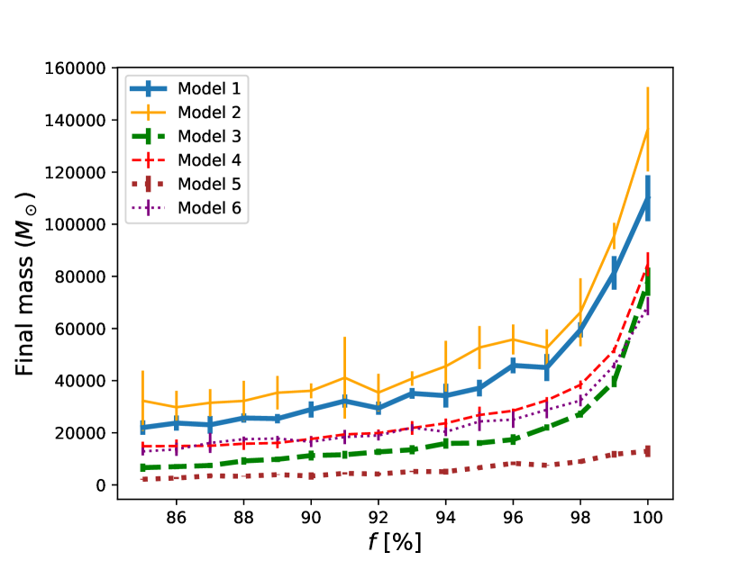
Figure 5: Final mass of the most massive object at the end of each simulation, as a function of the retained mass fraction $f$, for each model described. The bar at each point simulated represents the $\sigma$ error considering 5 simulations for each $f$ per model.

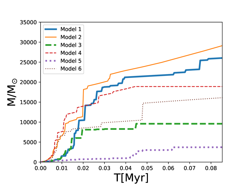
Figure 6: Time evolution of the mass of the central object, for six different accretion models and a 10% mass loss per collision. All models, except for number 5, efficiently convert gas mass into one massive object.

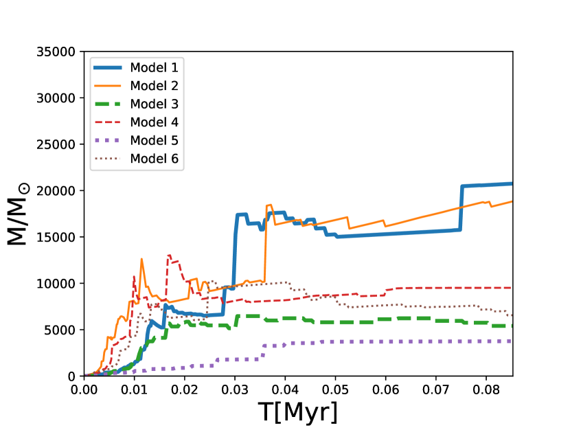
Figure 7: Same as Fig. 8, but in a scenario that allows for a decrease in the mass after a collision. Models 1 and 2 efficiently convert gas into one massive object, the efficiency of the other models is lower than in the other scenario.

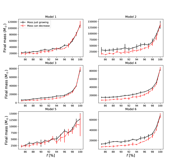
Figure 8: Comparison of models where the mass of the most massive object can only increase (black line) after a collision, and models that allow a decreasing mass (red). Each point in each plot has a bar representing the $\sigma$ error considering 5 simulations for each retained mass fraction $f$ per model.

The main goal of our simulations is to better understand how the mass of the central object in the cluster changes when mass loss is considered. In the first simulations, we considered constant values for the factor $f$ that regulates mass loss during collisions, and studied how the cluster evolves.

The simulations start with a cluster of single protostars. As the system evolves, different collision products will form. Also, dynamical encounters among protostars can eject them from the cluster. Thus we define four categories to which a protostar in the simulation can be part of: single protostar: which are part of the cluster but are not part of a collision product, the most massive collision product, a less massive collision product, and an escaper: which are stars that are far away from the cluster with positive energy. Figure 1 presents the time evolution of the fraction of protostars belonging to each of the defined categories, for the position independent models (1, 3 and 5), which represent the different kind of behaviors for every model. The majority of protostars end up in the final most massive object for models 1 and 3, while most of the stars do not undergo merger events in model 5. In the first models, as a result of gas accretion, the protostars are growing in radius, because protostellar mass is also increasing, thus getting a larger cross-section, resulting in a high collision probability in this environment. As we decrease the value of $f$, the fraction of objects that become part of the most massive object decreases, but the number of protostars that escape, or take part in a less massive collision product increases, as a result of the mass. In model 5, because of the uniform accretion, the central object in this model is less massive, and due to the time-dependent accretion, the protostellar radii shrink again as the cluster runs out of gas. We observe that most of the stars remain single, and we see a higher fraction of escapers than in the other models; as we decrease $f$, the fraction of single stars becomes higher while the other fractions decrease. We can also say that inflated radii turn ejection events into collisions.

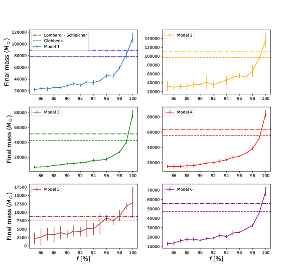
Figure 9: Results of simulations using the mass loss prescriptions by Lombardi and Glebbeek, compared with the mass loss just considering a constant retained mass fraction f $f$. The dashed line in each plot represents the simpler prescription given by equation (2), meanwhile the dash-dotted line represents the results of the more complex parametrization using the Schleicher et al. (2013) mass-radius relationship and the equation (1). Each line represents the mean of final mass for 5 simulations.

Figures 2, 3, and 4, present the collision rate (bottom panels) and correlate it with the total star and gas mass (top panels), the fraction of stars belonging to the four categories defined earlier (second panels), and the radius of the most massive protostar and the average radius of all the remaining protostars (third panels), for the three position independent models 1, 3, and 5, using $f$ = 0.9, 0.96 and 1. From Boekholt et al. (2018) the initial crossing time for a system with our parameter values is 853 yr, and in every model the collision rate starts to increase rapidly on a timescale of the order of 10⁴ years after the simulation has begun, which is equivalent to nearly a dozen crossing times, as well as a short time span compared to the total duration of the simulation. This timescale corresponds to the time it takes for the protostars to gain mass and obtain a larger radius, and also for the total stellar mass to be comparable to the gas mass. After reaching its peak, the collision rate decreases steadily and a small amount of objects starts to escape. The protostars grow rapidly and make the system stellar-mass dominated, producing dynamical encounters and collisions. For model 1 we find that the stars have a tendency to form a massive central object, with a low rate of escapers through the simulation. Model 3 presents an equally efficient way to form a massive object, but the rate of escapers is higher, especially at later times. Model 5 forms an object of moderate mass, and presents a steady escape rate.

The comparison between the scenarios with different values of $f$ is clear. A lower value of $f$ corresponds to a lower value in the total stellar mass of the system, and a lower fraction of the number of stars that form the most massive object in the cluster, also increasing the number of objects that escape. The average radius of the stars does not seem to be affected, but it is clear that the radius of the most massive object decreases with $f$. The largest difference is seen between $f$ values of 0.96 and 1. For 0.9 and 0.96, while there are differences, they are more subtle and not as important, which suggests that in this range of higher mass loss the simulations evolve in a similar way, so changing the value of $f$ is not as fundamental in this regime.

Now, to understand the effect on the final mass of the central object, we show the final mass as a function of $f$ in Fig. 5. We find that for models 1 and 2 the behavior of the curve changes abruptly when $f$ reaches a value of $\sim$0.96, for models 3, 4 and 6 there is also a sudden change of behavior around the same value. However, it is not as steep as the first one, and for model 5 there is no abrupt global change in the behavior of the plot, this can be seen in the Fig 5. With these observations we can say that there is a steep dependence on $f$ in the interval $f=[0.96-1.00]$, where the mass of the final object changes extremely with the value of $f$, so that even a small mass loss fraction is still relevant, obtaining values of almost one third of the mass obtained in simulations where mass loss is not considered. On the other hand, in the range $f=[0.85,0.96]$, changes in the value of $f$ do not lead to a big change in the final mass obtained. This suggests that, when considering a constant mass loss per collision, there is a breaking point where the mass loss fraction is a deciding factor in the resulting final mass of the most massive object.

In order to explain the change of behavior when we approach values of $f$ of $\sim 0.96$, we note that the typical masses of the protostars, around the final stages when they collide, are between $500-1000M_{\odot}$, while the central object has a mass of the order of several $10^{5}M_{\odot}$, therefore the mass loss is comparable to the mass gain during the collision, reducing the net effect. Considering the accretion rate, mass increases by about $300M_{\odot}$ in 0.01 Myr, so for this range of values of $f$ the mass loss during collisions with the massive object becomes comparable to the mass that has previously been accreted. We can say that for high values of $f$, the growth of the mass is dominated by collisions, and for lower values, it is dominated by accretion.

Also, we contrast scenarios where the mass of the most massive object can only increase after a collision, and scenarios that allow for a decrease. First, we compare the efficiency of the models to produce a massive object on a given timescale for a constant mass loss of 10%, as this represents a lower limit in the literature, for both scenarios. Figures 7 and 7, show the growth of the most massive object for these scenarios, demonstrating that when allowing for the mass to decrease after a collision, the efficiency to create a massive object decreases. We show the dependence on $f$ for the final mass for both scenarios, for each model, in Fig. 8. Due to the nature of our mass loss equation 1, when $f$ approaches 1 the mass we are going to obtain is the same as if we do not consider mass loss at all in the simulations, regardless of the kind of scenario we are in, so it is to be expected that both types of simulations behave the same at the higher end of the plot. What we see is that both types of simulations behave almost exactly the same for most of the models, for values of $f$ in the interval [0.96, 1]; both kind of simulations give similar final masses. This coincides with the range in which a small change in $f$ becomes relevant for the final mass. In particular we note that in models 1 and 3 there is little difference between the scenarios across all the values of $f$ tested, while in models 2, 4 and 6 the difference between these scenarios is more notorious for values of $f$ lower than 0.96, and model 3 exhibits a more erratic behavior at the higher end of the plot, but the masses obtained for both models are in the same range. This tells us that in the range where changes in $f$ are crucial, the results do not sensitively depend on the type of model, but for lower values of $f$, there are distinguishable differences, particularly for position dependent accretion models, as that in this regime the infrequent collisions may even remove some of the mass that has been accreted before.

Finally, we compare the results of the simulations with the parametrizations of Lombardi et al. (2002) and Glebbeek & Pols (2008). These parametrizations provide a single value for the mass obtained for each model, and we compare this value with the results of the simulations employing constant mass loss fractions, so we could see in which range we can consider the prescriptions to be equivalent to a constant mass loss scenario. Figure 9 shows the results we get for both analytical models, compared with the result we previously had in the constant mass loss scenario, for each accretion model. In general, the trend is that the prescriptions can be compared to a constant mass loss configuration where $f\sim 0.99$, nonetheless the exact value differs with the accretion model we consider. We also note that the parametrization using the Schleicher et al. (2013) protostellar models gives slightly higher values for the final mass than the simpler prescription by Glebbeek & Pols (2008), and the dispersion between them depends also on the accretion model we consider. The final mass values obtained from these simulations, including the calculated value of $f$ that would give that same mass in a constant mass loss scenario, and the corresponding percentage of the mass it represents when compared to models without mass loss are shown in Table 2.

Table 2: Overview of the results using the Lombardi and Glebbeek parametrizations, combined with the protostellar structure model by Schleicher et al. (2013) , including final mass, calculated $f$ value, and percentage of the mass compared to a scenario without mass loss.

	Glebbeek			Lombardi - Schleicher
Model	Mass ($M_{\odot}$)	$f$	%	Mass ($M_{\odot}$)	$f$	%
1	78003	98.84	74	89151	99.33	85
2	96714	99.03	70	109889	99.35	80
3	42214	99.06	54	51240	99.30	65
4	55610	99.12	65	63185	99.34	74
5	7683	97.11	59	8737	97.83	67
6	46980	99.05	68	55595	99.42	81

4 Summary and Conclusions

We have presented a study of how the mass loss during collisions can affect the final mass during the formation of SMBH seeds, formed through collisions and accretion, in a dense, primordial Pop. III protostellar cluster. We take into account standard cluster parameters as introduced by Boekholt et al. (2018), which ensure the production of massive black hole seeds. We investigated the effect of a constant fraction of mass loss per collision, for later comparison with more complex prescriptions. For that, we performed a series of simulations using the AMUSE framework, which included $N$-body dynamics, an analytical gas potential, different accretion models, mass-radius parametrizations, and stellar collisions.

First, we present the time evolution of the stellar components of the cluster for representative accretion models in Figure 1, which shows that for higher mass loss, the fraction of stars which become part of the most massive object decreases, while the single stars and escaper fraction gets larger, due to the fact that the cluster gravitational potential becomes smaller when mass loss increases.

In Figure 5 we present the results of our first simulations, showing the dependence of the final mass of the most massive object with the factor $f$ that describes mass loss. We can clearly see two distinct behaviors, for higher values of $f$ the mass depends steeply on its value, while for lower values the final mass does not change much with $f$, this can be explained because at the higher end of the plot the growth of the mass is dominated by collisions, and accretion dominates for the lower end. Figure 8 compares scenarios where the mass of the most massive object can only increase after a collision and scenarios that allow for a decrease, where we see that the differences between scenarios are more significant for lower values of $f$, while for higher values there is not much difference. This shows that in the range where changes in $f$ are important, whether or not we allow for the mass of an object to decrease after a collision is not really relevant. In this context, a constant mass loss of 5% represents a final mass between 60-80% lower (50% for model 5) than the mass we would get if we did not consider mass loss in our models.

Also, we compared the results of the constant mass loss simulations with more complex mass loss parametrizations by Lombardi et al. (2002) and Glebbeek & Pols (2008), using the Schleicher et al. (2013) mass-radius relationships for primordial protostars. The values obtained tell us that these analytical models are equivalent to scenarios of constant mass loss of $\sim$1% per collision. However, this low mass loss percentage can have a great impact on the final mass of the object, that could lose between 15 to 40% of its mass depending on the accretion model we study. Considering this, even in the most extreme mass loss scenarios, we get final masses of the order of $10^{4}M_{\odot}$, which can be considered massive enough to be SMBH seeds, confirming that the model is still a viable candidate for explaining the SMBH we see nowadays.

The mass loss in collisions of primordial protostars has not been studied, and given the importance of mass loss in the context of the formation of SMBH seeds, it is important to explore this in more detail in the future via hydrodynamical simulations, considering also three-body mergers and different relative velocities, with the aim to derive approximate relations that can subsequently be employed in $N$-body models. More precise models will help us better understand how we can really form the massive black holes we see today.

Appendix A

Table 3: Average final masses of the most massive object, obtained in simulations for constant $f$, and the percentage they represent of the most massive result

	Model 1		Model 2		Model 3		Model 4		Model 5		Model 6
$100f$	Mass ($M_{\odot}$)	%	Mass ($M_{\odot}$)	%	Mass ($M_{\odot}$)	%	Mass ($M_{\odot}$)	%	Mass ($M_{\odot}$)	%	Mass ($M_{\odot}$)	%
85	22009	21	32290	23	6627	8	14840	17	2178	16	12862	18
86	23731	22	29803	21	7021	9	14927	17	2642	20	13652	19
87	23059	22	31503	23	7456	9	15027	17	3479	26	16112	23
88	25666	24	32230	23	9209	11	15810	18	3332	25	17559	25
89	25428	24	35371	25	9826	12	16099	19	3943	30	17791	25
90	28942	27	36110	26	11274	14	17651	20	3429	26	16561	24
91	32182	30	41123	30	11586	14	19384	22	4439	34	18374	26
92	29457	28	35436	25	12674	16	19912	23	4186	32	18982	27
93	35107	33	40799	29	13496	17	21854	25	5157	39	21958	32
94	34242	32	45533	33	15921	20	23655	27	5092	39	20362	29
95	37147	35	52715	38	16082	20	26838	31	6621	51	24351	35
96	45838	43	55783	40	17400	22	28448	33	8287	64	25074	36
97	45031	43	52618	38	22053	28	32457	38	7515	58	28820	42
98	59486	56	66223	48	27167	34	38402	45	8971	69	32367	47
99	81334	77	95491	69	39667	50	51641	60	11760	90	45806	66
100	104674	100	136457	100	77962	100	84671	100	12925	100	68615	100

In table 3 is an overview of the results of all the simulations, for all the models studied, considering a constant mass loss, given by the value of $f$, which represents the fraction of mass that remains after a collision. The table shows the value of the final mass for the most massive object at the end of the simulation, and the percentage that the mass represents in comparison to the final mass when no mass loss is considered. All the values for mass on the table are averages.

References

- Agarwal & Khochfar (2014) Agarwal B., Khochfar S., 2014, MNRAS, 446, 160
- Agarwal et al. (2017) Agarwal B., Cullen F., Khochfar S., Klessen R. S., Glover S. C. O., Johnson J., 2017, MNRAS, 468, L82
- Bañados et al. (2018) Bañados E., et al., 2018, Nature, 553, 473
- Baumgardt & Klessen (2011) Baumgardt H., Klessen R. S., 2011, Monthly Notices of the Royal Astronomical Society, 413, 1810–1818
- Boekholt et al. (2018) Boekholt T. C. N., et al., 2018, MNRAS, 476, 366
- Bovino et al. (2014) Bovino S., Grassi T., Schleicher D. R. G., Latif M. A., 2014, ApJL, 790, L35
- Bovino et al. (2016) Bovino S., Grassi T., Schleicher D. R. G., Banerjee R., 2016, ApJ, 832, 154
- Bromm & Loeb (2003) Bromm V., Loeb A., 2003, ApJ, 596, 34
- Dale & Davies (2006) Dale J. E., Davies M. B., 2006, MNRAS, 366, 1424–1436
- Devecchi & Volonteri (2009) Devecchi B., Volonteri M., 2009, ApJ, 694, 302
- Devecchi et al. (2012) Devecchi B., Volonteri M., Rossi E. M., Colpi M., Portegies Zwart S., 2012, MNRAS, 421, 1465
- Dijkstra et al. (2014) Dijkstra M., Ferrara A., Mesinger A., 2014, MNRAS, 442, 2036
- Dopcke et al. (2013) Dopcke G., Glover S. C. O., Clark P. C., Klessen R. S., 2013, ApJ, 766, 103
- Fujii et al. (2007) Fujii M., Iwasawa M., Funato Y., Makino J., 2007, PASJ, 59, 1095
- Gaburov et al. (2008) Gaburov E., Lombardi J. C. J., Portegies Zwart S., 2008, MNRAS, 383, L5–L9
- Gaburov et al. (2010) Gaburov E., Lombardi J. C., Zwart S. P., 2010, MNRAS, 402, 105
- Glebbeek & Pols (2008) Glebbeek E., Pols O. R., 2008, A&A, 488, 1017
- Hosokawa et al. (2012) Hosokawa T., Omukai K., Yorke H. W., 2012, ApJ, 756, 93
- Katz et al. (2015) Katz H., Sijacki D., Haehnelt M. G., 2015, MNRAS, 451, 2352
- Latif et al. (2013) Latif M. A., Schleicher D. R. G., Schmidt W., Niemeyer J., 2013, MNRAS, 433, 1607–1618
- Latif et al. (2014) Latif M. A., Schleicher D. R. G., Bovino S., Grassi T., Spaans M., 2014, ApJ, 792, 78
- Latif et al. (2015) Latif M. A., Bovino S., Grassi T., Schleicher D. R. G., Spaans M., 2015, MNRAS, 446, 3163
- Lombardi et al. (2002) Lombardi Jr. J. C., Warren J. S., Rasio F. A., Sills A., Warren A. R., 2002, ApJ, 568, 939–953
- Mayer et al. (2013) Mayer L., Latif M., Schleicher D. R. G., 2013, Formation of the First Black Holes, pp 195–228
- Mortlock et al. (2011) Mortlock D. J., et al., 2011, Nature, 474, 616–619
- Pelupessy et al. (2013) Pelupessy F. I., van Elteren, A. de Vries, N. McMillan, S. L. W. Drost, N. Portegies Zwart, S. F. 2013, A&A, 557, A84
- Portegies Zwart & McMillan (2018) Portegies Zwart S., McMillan S., 2018, Astrophysical Recipes; The art of AMUSE, doi:10.1088/978-0-7503-1320-9.
- Portegies Zwart et al. (2009) Portegies Zwart S. F., et al., 2009, New Astron., 14, 369
- Portegies Zwart et al. (2013) Portegies Zwart S., McMillan S., van Elteren A., Pelupessy F., de Vries N., 2013, Comput. Phys. Com., 184, 456
- Rees (1984) Rees M. J., 1984, ARA&A, 22, 471
- Reinoso et al. (2018) Reinoso B., Schleicher D., Fellhauer M., Klessen R., Boekholt T. C. N., 2018, A&A, 614, A14
- Sakurai et al. (2017) Sakurai Y., Yoshida N., Fujii M. S., Hirano S., 2017, MNRAS, 472, 1677
- Schleicher et al. (2013) Schleicher D., Palla F., Ferrara A., Galli D., Latif M., 2013, A&A, 558
- Schneider et al. (2006) Schneider R., Omukai K., Inoue A. K., Ferrara A., 2006, MNRAS, 369, 1437
- Shang et al. (2010) Shang C., Bryan G. L., Haiman Z., 2010, MNRAS, 402, 1249
- Shapiro (2005) Shapiro S. L., 2005, ApJ, 620, 59
- Suazo et al. (2019) Suazo M., Prieto J., Escala A., Schleicher D., 2019, ApJ
- Sugimura et al. (2014) Sugimura K., Omukai K., Inoue A. K., 2014, MNRAS, 445, 544
- Wise et al. (2008) Wise J. H., Turk M. J., Abel T., 2008, ApJ, 682, 745
- Woods et al. (2018) Woods T. E., et al., 2018, PASA, 36