Space time stabilized finite element methods for a unique continuation problem subject to the wave equation

Abstract.

We consider a stabilized finite element method based on a spacetime formulation, where the equations are solved on a global (unstructured) spacetime mesh. A unique continuation problem for the wave equation is considered, where data is known in an interior subset of spacetime. For this problem, we consider a primal-dual discrete formulation of the continuum problem with the addition of stabilization terms that are designed with the goal of minimizing the numerical errors. We prove error estimates using the stability properties of the numerical scheme and a continuum observability estimate, based on the sharp geometric control condition by Bardos, Lebeau and Rauch. The order of convergence for our numerical scheme is optimal with respect to stability properties of the continuum problem and the interpolation errors of approximating with polynomial spaces. Numerical examples are provided that illustrate the methodology.

1. Introduction

We consider a data assimilation problem for the acoustic wave equation, formulated as follows. Let $n\in\{1,2,3\}$, $T>0$ and $\Omega\subset\mathbb{R}^{n}$ be an open, connected, bounded set with smooth boundary $\partial\Omega$. Let $u$ be the solution of the initial boundary value problem

(1.1) $$\begin{cases}\Box u=\partial_{t}^{2}u-\Delta u=0,&\text{on $\mathcal{M}=(0,T)\times\Omega$},\\ u=0,&\text{on $\Sigma=(0,T)\times\partial\Omega$},\\ u|_{t=0}=u_{0},\ \partial_{t}u|_{t=0}=u_{1}&\text{on $\Omega$}.\end{cases}$$

The initial data $u_{0},u_{1}$ are assumed to be a priori unknown functions, but the measurements of $u$ in some spacetime subset $\mathcal{O}=(0,T)\times\omega$, where $\omega\subset\overline{\Omega}$ is open, is assumed to be known:

(1.2) $$u|_{\mathcal{O}}=u_{\mathcal{O}}.$$

The data assimilation problem then reads as follows:

(DA) Find $u$ given $u_{\mathcal{O}}$.

The existence of a solution to the 1 problem is always implicitly guaranteed in the sense that the measurements $u_{\mathcal{O}}$ correspond to a physical solution to the wave equation (1.1). On the other hand, assuming that

(1.3) $$T>2\max\{\operatorname{dist}(x,\omega)\,|\,x\in\overline{\Omega}\},$$

it follows from Holmgren’s unique continuation theorem that the solution to 1 is unique. Although uniquely solvable, 1 might have poor stability properties if only (1.3) is assumed. We will require the 1 problem to be Lipschitz stable, and for this reason we make the stronger assumption that the so-called geometric control condition holds. This condition originates from [BLR88, BLR92] and we refer the reader to these works for the precise definition. Roughly speaking, the condition requires that all geometric optic rays in $\mathcal{M}$, taking into account their reflections at boundary, intersect the set $(0,T)\times\omega$.

We recall the following formulation of the observability estimates appearing in [BLR92, Theorem 3.3] and [LRLTT17, Proposition 1.2]. For the explicit derivation of this version of the estimate, we refer the reader to [BFO18, Theorem 2.2].

Theorem 1.

Let $\omega\subset\overline{\Omega}$, $T>0$ and suppose that $(0,T)\times\omega$ satisfies the geometric control condition. If $u(0,\cdot)\in L^{2}(\Omega)$, $\partial_{t}u(0,\cdot)\in H^{-1}(\Omega)$, $u|_{(0,T)\times\partial\Omega}\in L^{2}(\Sigma)$, and $\Box u\in H^{-1}(\mathcal{M})$, then

$$u\in C^{1}([0,T];H^{-1}(\Omega))\cap C([0,T];L^{2}(\Omega)),$$

and

$$\sup_{t\in[0,T]}\biggl{(}\|u(t,\cdot)\|_{L^{2}(\Omega)}+\|\partial_{t}u(t,\cdot)\|_{H^{-1}(\Omega)}\biggr{)}\leqslant C\left(\|u\|_{L^{2}(\mathcal{O})}+\|\Box u\|_{H^{-1}(\mathcal{M})}+\|u\|_{L^{2}(\Sigma)}\right),$$

where $C>0$ is a constant depending on $\mathcal{M}$ and $\omega$.

Let us remark that the geometric control condition is sharp in the sense that Theorem 1 fails to hold if the geometric control condition does not hold on the set $(0,T)\times\omega$ [BLR88].

The objective of the paper is to design a stabilized spacetime finite element method for the data assimilation problem 1, which allows for higher order approximation spaces. The method will also allow for an error analysis exploiting the stability of Theorem 1 and the accuracy of the spaces in an optimal way. To the best of our knowledge this is the first complete numerical analysis of the data assimilation problem for the wave equation, using high order spaces.

1.1. Previous literature

Spacetime methods for inverse problems subject to the wave equation were introduced in [CM15a] with an application to the control problem in [CM15b]. In those works however, the required $H^{2}$ regularity of the constraint equation was respected on the level of approximation leading to an approach using $C^{1}$-continuous approximation spaces in spacetime. Herein we instead use an approach where the approximating space is only $H^{1}$-conforming and we handle instabilities arising due to the lack of conformity of the space through the addition of stabilization terms. This approach to stabilization of ill-posed problems draws on the works [Bur13, Bur14], for the elliptic Cauchy problem. In the context of time dependent problems, unique continuation for the heat equation was considered in [BO18, BIHO18], with piecewise affine finite elements in space and finite differences for the time discretization. Finally using a similar low order approach, with conventional, finite difference type time-discretization, the unique continuation and control problems for the wave equation were considered in [BFO18] and [BFO19] respectively. Another strategy requiring only $H^{1}$-regularity consists in reformulating the second order wave equation as a first order system; it is examined in [MM19] for the corresponding controllability problem.

The upshot in the present work is that by using the spacetime framework, we may very easily design a method that allows for high order approximation spaces with provable, close to optimal, convergence rates, without resorting to $C^{1}$-type approximation spaces.

There are several works that approach the data assimilation problem (DA), or its close variants, by solving a sequence of classical initial–boundary value problems for the wave equation. Such methods have been proposed independently in [SU09], in the context of a particular application to Photoacoustic tomography, and in [RTW10], based on the so-called Luenberger observers algorithm first introduced in an ODE context in [AB05]. An error estimate for a discretization of a Luenberger observers based algorithm was proven in [HR12], giving logarithmic convergence rate with respect to the mesh size. Better convergence rates can be proven if a stability estimate is available on a scale of discrete spaces. Such discrete estimates were first derived in [IZ99] and we refer the reader to the survey articles [Zua05, EZ12] and the monograph [EZ13], as well as the recent paper [EMZ16] for more details. Optimal-in-space discrete estimates can be derived from continuous estimates [Mil12], however, spacetime optimal discrete estimates are known only for specific situations.

The data assimilation problem (DA) can also be solved using the quasi-reversibility method. This method originates from [LL67], and it has been applied to data assimilation problems subject to the wave equation in [KM91, KR92], and more recently to the Photoacoustic tomography problem in [CK08]. We are not aware of any works proving sharp convergence rates for the quasi-reversibility method with respect to mesh size.

The data assimilation problem (DA) arises in several applications. We mentioned already Photoacoustic tomography (PAT), and refer to [Wan09] for physical aspects of PAT, to [KK08] for a mathematical review, and to [AM15, CO16, NK16, SY15] for the PAT problem in a cavity, the case closest to (DA). Another interesting application is given in [BPD19] where an obstacle detection problem is solved by using a level set method together with the quasi-reversibility method applied to a variant of (DA).

1.2. Outline of the paper

The paper is organized as follows. In Section 2 we introduce a few notations used in the paper. In Section 3, we start by introducing the mixed spacetime mesh followed by the discrete representation of 1 in terms of a primal dual Lagrangian formulation. The Euler-Lagrange equations are studied, showing in particular that there exists a unique solution to the discrete formulation of 1. Section 4 is concerned with proving the convergence rates for the numerical error functions corresponding to the primal and dual variables. Finally, in Section 5 we provide two numerical examples that illustrate the theory while also making a comparison with the $H^{2}$-conformal finite element method introduced in [CM15a].

2. Notations

We write $\nabla_{t,x}u=(\partial_{t}u,\nabla u),$ where $\nabla u\in\mathbb{R}^{n}$ is the usual gradient with respect to the space variables. The wave operator may be written as

$$\Box u=-\nabla_{t,x}\cdot(A\nabla_{t,x}u),$$

where $A$ is the matrix associated to the Minkowski metric in $\mathbb{R}^{1+n}$, that is,

$$A=\left[\begin{array}[]{cc}-1&0_{[1,n]}\\ 0_{[n,1]}&\mathbb{I}_{[n,n]}\end{array}\right]$$

with $\mathbb{I}_{[n,n]}$ denoting the $n\times n$ identity matrix. We introduce the notations

$$(u,v)_{\mathcal{M}}=\int_{0}^{T}\!\!\!\int_{\Omega}u(t,x)v(t,x)\,dx\,dt,\quad\|u\|_{\mathcal{M}}=(u,u)^{\frac{1}{2}}_{\mathcal{M}}$$

and

$$(u,v)_{\mathcal{O}}=\int_{0}^{T}\!\!\!\int_{\omega}u(t,x)v(t,x)\,dx\,dt,\quad\|u\|_{\mathcal{O}}=(u,u)^{\frac{1}{2}}_{\mathcal{O}}$$

and use an analogous notation for inner products over other subsets of $\overline{\mathcal{M}}$, with the understanding that the natural volume measures are used in the case of subdomains. We also use the shorthand notation

$$a(u,z)=(A\nabla_{t,x}u,\nabla_{t,x}z)_{\mathcal{M}},$$

and note in passing that given any $(u_{0},u_{1})\in H^{1}_{0}(\Omega)\times L^{2}(\Omega)$, the solution $u$ to equation (1.1) satisfies

$$a(u,v)=0,\quad\forall v\in H^{1}_{0}(\mathcal{M}).$$

Finally, we fix an integer $p$, and make the standing assumption that the continuum solution $u$ to 1 satisfies

$$u\in H^{p+1}(\mathcal{M})\quad\text{for some $p\in\mathbb{N}$}.$$

The index $p$ defined above will correspond to the highest order of the spacetime polynomial approximations that can be used for the discrete solution to 1, while still getting optimal convergence for the numerical errors.

3. Discrete formulation of the data assimilation problem

Let us start this section by observing that the solution $u$ to the data assimilation problem 1 can be obtained by analyzing the saddle points for the continuum Lagrangian functional $\mathcal{J}(u,z)$ that is defined through

$$\mathcal{J}(u,z)=\frac{1}{2}\|u-q\|^{2}_{\mathcal{O}}+a(u,z),$$

for any

$$u\in H^{1}(0,T;L^{2}(\Omega))\cap L^{2}(0,T;H^{1}_{0}(\Omega))\quad\text{and}\quad z\in H^{1}_{0}(\mathcal{M}).$$

Here, the wave equation is imposed on the primal variable $u$ by introducing a Lagrange multiplier $z$. It is easy to verify the the solution $u$ to 1 together with $z=0$ is a saddle point for the Lagrangian functional.

Motivated by this example, we would like to present a discrete Lagrangian functional to numerically solve 1. We will use discrete stabilizer (also called regularizer) terms that guarantee the existence of a unique critical point. These terms will be designed with the goal of minimizing the numerical error functions for the primal and dual variables.

We begin by introducing the spacetime mesh in Section 3.1. Then a discrete version of the bi-linear functional $a(\cdot,\cdot)$ is provided in Section 3.2, followed by the introduction of the stabilization terms in Section 3.3. Finally, we present the discrete formulation of 1 in Section 3.4.

3.1. Spacetime discretization

In this section we will introduce the spacetime finite element method that we propose. The method is using an $H^{1}$-conforming piecewise polynomial space defined on a spacetime triangulation that can consist of simplices, or prisms. Herein for simplicity we restrict the discussion to the simplicial case. To be able to handle the case of curved boundaries without complicating the theory with estimations of the error in the approximation of the geometry we impose boundary conditions using a technique introduced by Nitsche [Nit71]. See also [Tho97, Theorem 2.1] for a discussion of the application of the method to curved boundaries.

Consider a family $\mathcal{T}=\{\mathcal{T}_{h};\ h>0\}$ of quasi uniform triangulations of $\mathcal{M}$ consisting of simplices $\{K\}$ such that the intersection of any two distinct simplices is either a common vertex, a common edge or a common face. We let $h_{K}=\mbox{diam}(K)$ and $h=\max_{K\in\mathcal{T}}h_{K}$, (see e.g. [EG04, Def. 1.140]). By quasi-uniformity $h/h_{K}$ is uniformly bounded, and therefore for simplicity the quasi-uniformity constant will be set to one below. Observe that we do not consider discretization of the smooth boundary $\partial\mathcal{M}$, but instead we allow triangles adjacent to the boundary to have curved faces, fitting $\mathcal{M}$. Finally, given any $k\in\mathbb{N}$, we let $V^{k}_{h}$ be the $H^{1}(\mathcal{M})$-conformal approximation space of polynomial degree less than or equal to $k$, that is,

(3.1) $$V^{k}_{h}=\{u\in C(\mathcal{M}):\ u|_{K}\in\mathbb{P}_{k}(K),\ \forall K\in\mathcal{T}_{h}\},$$

where $\mathbb{P}_{k}(K)$ denotes the set of polynomials of degree less than or equal to $k\geq 1$ on $K$.

Next, we record two inequalities that will be used in the paper. The family $\mathcal{T}$ satisfies the following trace inequality, see e.g. [BS08, Eq. 10.3.9],

(3.2) $$\|u\|_{L^{2}(\partial K)}\lesssim h^{-\frac{1}{2}}\|u\|_{L^{2}(K)}+h^{\frac{1}{2}}\|\nabla u\|_{L^{2}(K)},\quad u\in H^{1}(K),$$

The family $\mathcal{T}$ also satisfies the following discrete inverse inequality, see e.g. [EG04, Lem. 1.138],

(3.3) $$\|\nabla u\|_{L^{2}(K)}\lesssim h^{-1}\|u\|_{L^{2}(K)},\quad u\in\mathbb{P}_{p}(K).$$

Remark 1.

We will use the notations $A\lesssim B$ (resp., $A\gtrsim B$) to imply that there exists a constant $C>0$ independent of the spacetime mesh parameter $h$, such that the inequalities $A\leqslant CB$ (resp., $A\geqslant CB$) hold.

Remark 2.

It is also possible to consider the space $V^{k}_{h}\cap C^{1}(\mathcal{M})$ with $k\geqslant 2$, for the approximation of the primal variable. In this case the method coincides with that of [CM15a] and the analysis shows that optimal error estimates are satisfied also in this case.

Remark 3.

We will use the approximation space $V_{h}^{p}$ for the primal variable $u$. We will also fix an integer $q\leqslant p$ and use the space $V_{h}^{q}$ for the approximation of the dual variable $z$. As we will see, using our method, the approximation space of the dual variable can be quite coarse without sacrificing any rate of convergence for the discrete primal variable (i.e we can take $q=1$).

3.2. A discrete bi-linear formulation for the wave equation

Since no boundary conditions are imposed on the space $V^{p}_{h}$, the form $a(u,z)$ needs to be modified on the discrete level. For the formulation to remain consistent we propose the following modified bilinear form on $V^{p}_{h}\times V^{q}_{h}$,

$$a_{h}(u_{h},z_{h})=a(u_{h},z_{h})-(A\nabla_{t,x}u_{h}\cdot n_{\partial\mathcal{M}},z_{h})_{\partial\mathcal{M}}-(\nabla z_{h}\cdot n_{\partial\Omega},u_{h})_{\Sigma}.$$

Here $n_{\partial\mathcal{M}}$ and $n_{\partial\Omega}$ are the outward unit normal vectors on $\partial\mathcal{M}$ and $\partial\Omega$ respectively. The last term in the right hand side is added to make the weak form of the Laplace operator symmetric even in the case where no boundary conditions are imposed on the discrete spaces. Depending on how the stabilizing terms are chosen below, this term is not strictly necessary in this work, but becomes essential if the formulation must be consistent also for the adjoint equation.

Observe that, using integration by parts, there holds

(3.4) $$a_{h}(u,z_{h})=(\Box u,z_{h})_{\mathcal{M}}-\underbrace{(\nabla z_{h}\cdot n_{\partial\Omega},u)_{\Sigma}}_{=0}=(\Box u,z_{h})_{\mathcal{M}}$$

for all $u\in H^{2}(\mathcal{M})\cap L^{2}(0,T;H^{1}_{0}(\Omega))$.

3.3. Formulation of the discrete stabilization terms for primal and dual variables

We denote by $\mathcal{F}_{h}$ the set of internal faces of $\mathcal{T}_{h}$, and define for $F\in\mathcal{F}_{h}$, the jump of a scalar quantity $u$ over $F$ by

$$\llbracket u\rrbracket_{F}=u|_{K_{1}}-u|_{K_{2}}$$

where $K_{1},K_{2}\in\mathcal{T}_{h}$ are the two simplices satisfying $K_{1}\cap K_{2}=F$. For vector valued quantities $u$ we define

$$\llbracket n\cdot u\rrbracket_{F} =n_{1}\cdot u|_{K_{1}}+n_{2}\cdot u|_{K_{2}},$$

where $n_{j}$ is the outward unit normal vector of $K_{j}$, $j=1,2$. Sometimes we drop the normal to alleviate the notation. The norm over all the faces in $\mathcal{F}_{h}$ will be denoted by

$$\|v\|_{\mathcal{F}_{h}}=\left(\sum_{F\in\mathcal{F}_{h}}\|v\|^{2}_{F}\right)^{\frac{1}{2}},$$

and the norm over all the simplices $\{K\}$ will be denoted by

$$\|v\|_{\mathcal{T}_{h}}=\left(\sum_{K\in\mathcal{T}_{h}}\|v\|_{K}^{2}\right)^{\frac{1}{2}}.$$

For each $K\in\mathcal{T}_{h}$, we define the elementwise stabilizing form

(3.5) $$s_{K}(u_{h},u_{h})=\|h\Box u_{h}\|_{K}^{2}+\|h^{-\frac{1}{2}}u_{h}\|_{\partial K\cap\Sigma}^{2}+\sum_{F\in\partial K\cap\mathcal{F}_{h}}\|h^{\frac{1}{2}}\llbracket A\nabla_{t,x}u_{h}\rrbracket\|_{F}^{2}.$$

A dual stabilizer is defined by

(3.6) $$s_{K}^{*}(z_{h},z_{h})=\|\nabla_{t,x}z_{h}\|_{K}^{2}+\|h^{-\frac{1}{2}}z_{h}\|^{2}_{\partial K\cap\partial\mathcal{M}}.$$

Subsequently, the global stabilizers are defined by summing over all the elements:

$$s=\sum_{K\in\mathcal{T}_{h}}s_{K}\quad\mbox{and}\quad s^{*}=\sum_{K\in\mathcal{T}_{h}}s^{*}_{K}$$

and we define the semi norms $|u|_{s}=s(u,u)^{\frac{1}{2}}$ and $|z|_{s^{*}}=s^{*}(z,z)^{\frac{1}{2}}$. Observe that the following stability estimate holds:

(3.7) $$|w_{h}|_{s^{*}}\lesssim\|\nabla_{t,x}w_{h}\|_{\mathcal{M}}+\|h^{-\frac{1}{2}}w_{h}\|_{\partial\mathcal{M}}\quad\forall\,w_{h}\in V_{h}^{q}.$$

We also point out for future reference that for a solution to the data assimilation problem $u\in H^{2}(\mathcal{M})$ and all $u_{h}\in V_{h}^{p}$, there holds

(3.8) $$s(u-u_{h},u-u_{h})=s(u_{h},u_{h}).$$

Remark 4.

There is some freedom in the choices of the discrete regularization terms that yield the same error estimates as in Theorem 2 below. The choice is more flexible for the dual variable $z$ since the continuum analogue for this variable is zero. For instance we can define the following stabilization term for the dual variable:

(3.9) $$s_{K}^{*}(z_{h},z_{h})=s_{K}(z_{h},z_{h})+\|h^{-\frac{1}{2}}z_{h}\|_{\partial K\cap(\partial\mathcal{M}\setminus\Sigma)}+\|h^{\frac{1}{2}}\partial_{t}z_{h}\|_{\partial K\cap(\partial\mathcal{M}\setminus\Sigma)}^{2}.$$

It is also possible to use a stabilization that is exclusively carried by the faces of the computational mesh provided $q\in\{p-2,p-1,p\}$. In this case we define

(3.10) $$s_{K}(u_{h},u_{h})=\sum_{F\in\partial K\cap\mathcal{F}_{h}}\left(\|h^{\frac{1}{2}}\llbracket A\nabla_{t,x}u_{h}\rrbracket\|_{F}^{2}+\|h^{\frac{3}{2}}_{F}\llbracket\Box u_{h}\rrbracket\|_{F}^{2}\right)+\|h^{-\frac{1}{2}}u_{h}\|_{\partial K\cap\Sigma}^{2}.$$

In the second jump term we are allowed to split the operator in the time derivative and the Laplace operator (or second order derivatives in space) without sacrificing stability or consistency since

$$\|h^{\frac{3}{2}}_{F}\llbracket\Box u_{h}\rrbracket\|_{F}^{2}\leqslant\|h^{\frac{3}{2}}_{F}\llbracket\partial_{t}^{2}u_{h}\rrbracket\|_{F}^{2}+\|h^{\frac{3}{2}}_{F}\llbracket\Delta u_{h}\rrbracket\|_{F}^{2}.$$

Weak consistency of the right order still holds since for a sufficiently smooth solution $u$

$$\|h^{\frac{3}{2}}_{F}\llbracket\partial_{t}^{2}u\rrbracket\|_{F}^{2}+\|h^{\frac{3}{2}}_{F}\llbracket\Delta u\rrbracket\|_{F}^{2}=0.$$

3.4. The discrete Lagrangian formulation for the data assimilation problem

Our finite element method is defined by the discrete Lagrangian functional

$$\mathcal{L}:V_{h}^{p}\times V_{h}^{q}\to\mathbb{R},$$

through

(3.11) $$\mathcal{L}(u,z)=\frac{1}{2}\|u-u_{\mathcal{O}}\|_{\mathcal{O}}^{2}+\frac{\gamma}{2}\,s(u,u)-\frac{\gamma^{*}}{2}\,s^{*}(z,z)+a_{h}(u,z),$$

where $\gamma,\gamma^{*}>0$ are fixed constants.

The corresponding Euler-Lagrange equations read as follows. Find $(u_{h},z_{h})\in V^{p}_{h}\times V^{q}_{h}$ such that for all $(v_{h},w_{h})\in V^{p}_{h}\times V^{q}_{h}$ there holds

(3.12) $$a_{h}(u_{h},w_{h})-\gamma^{*}s^{*}(z_{h},w_{h}) =0,$$

(3.13) $$(u_{h},v_{h})_{\mathcal{O}}+\gamma s(u_{h},v)+a_{h}(v_{h},z_{h}) =(u_{\mathcal{O}},v_{h})_{\mathcal{O}}.$$

To simplify the notation we introduce the bilinear form

$$\mathcal{A}_{h}[(u_{h},z_{h}),(v_{h},w_{h})]=(u_{h},v_{h})_{\mathcal{O}}+\gamma s(u_{h},v_{h})+a_{h}(v_{h},z_{h})+a_{h}(u_{h},w_{h})-\gamma^{*}s^{*}(z_{h},w_{h}).$$

The discrete problem (3.12)-(3.13) can then be recast as follows. Find $u_{h},z_{h}\in V^{p}_{h}\times V^{q}_{h}$ such that

(3.14) $$\mathcal{A}_{h}[(u_{h},z_{h}),(v_{h},w_{h})]=(u_{\mathcal{O}},v_{h})_{\mathcal{O}},\quad\forall(v_{h},w_{h})\in V^{p}_{h}\times V^{q}_{h}.$$

We note that by (3.8) and (3.4) there holds

(3.15) $$\mathcal{A}_{h}[(u-u_{h},z_{h}),(v_{h},w_{h})]=0.$$

Define the residual norm

$$|\|(u,z)\||^{2}_{S}=\|u\|_{\mathcal{O}}^{2}+|u|_{s}^{2}+|z|^{2}_{s^{*}},$$

and a continuity norm

$$\|u\|_{*}=\|\nabla_{t,x}u\|_{\mathcal{M}}+\|h^{\frac{1}{2}}A\nabla_{t,x}u\cdot n\|_{\partial\mathcal{M}}+\|h^{-\frac{1}{2}}u\|_{\Sigma}.$$

For the purpose of our error analysis later, we also introduce a family of interpolants $\pi^{k}_{h}$, that are required to satisfy

Assumption 1.

$\pi^{k}_{h}:H^{k}(\mathcal{M})\to V^{k}_{h}$ preserves Dirichlet boundary conditions and additionally satisfies

$$\|u-\pi^{k}_{h}u\|_{H^{m}(\mathcal{M})}\lesssim h^{s-m}\|u\|_{H^{s}(\mathcal{M})} u\in H^{s}(\mathcal{M}) s=0,1,\ldots,k+1 m=0,1,\ldots,s$$ for all with and .

An example of such an interpolant is the Scott-Zhang interpolant [SZ90]. For brevity, we will use the notations:

$$\pi_{h}=\pi^{1}_{h}\quad\text{and}\quad\Pi_{h}=\pi^{p}_{h}.$$

We have the following lemma regarding the residual norm:

Lemma 1.

Let $u\in H^{p+1}(\mathcal{M})$. There holds:

$$|\|(u-\Pi_{h}u,0)\||_{S}\lesssim h^{p}\|u\|_{H^{p+1}(\mathcal{M})},$$

Proof.

Note that

$$|\|(u-\Pi_{h}u,0)\||_{S}=\|u-\Pi_{h}u\|_{\mathcal{O}}+|u-\Pi_{h}u|_{s}.$$

For the first term we immediately see that

$$\|u-\Pi_{h}u\|_{\mathcal{O}}\leqslant\|u-\Pi_{h}u\|_{\mathcal{M}}\lesssim h^{p+1}\|u\|_{H^{p+1}(\mathcal{M})}.$$

To bound the contribution from the stabilization term, recall by definition that

$$|u-\Pi_{h}u|_{s}^{2}=\sum_{K\in\mathcal{T}_{h}}\left(\|h\Box(u-\Pi_{h}u)\|_{K}^{2}+\|h^{-\frac{1}{2}}(u-\Pi_{h}u)\|_{\partial K\cap\Sigma}^{2}+\sum_{F\in\partial K\cap\mathcal{F}_{h}}\|h^{\frac{1}{2}}\llbracket A\nabla_{t,x}(u-\Pi_{h}u)\rrbracket\|_{F}^{2}\right).$$

We proceed to bound the three terms on the right hand side. For the first term, we note that

$$\sum_{K\in\mathcal{T}_{h}}\|h\Box(u-\Pi_{h}u)\|_{K}^{2}\lesssim\sum_{K\in\mathcal{T}_{h}}\|\nabla_{t,x}(u-\Pi_{h}u)\|_{K}^{2}\lesssim h^{2p}\|u\|_{H^{p+1}(\mathcal{M})}^{2}.$$

For the second term, we define $\Delta_{F}=\{K:\bar{K}\cap F\neq\emptyset\}$, $\tilde{\Delta}_{F}=\{K:\bar{K}\cap\bar{\Delta}_{F}\neq\emptyset\}$ and use (3.2) to write

$$\|h^{-\frac{1}{2}}(u-\Pi_{h}u)\|^{2}_{F}\lesssim h^{-1}\|u-\Pi_{h}u\|^{2}_{\Delta_{F}}+\|\nabla_{t,x}(u-\Pi_{h}u)\|^{2}_{\Delta_{F}}\lesssim h^{2p}|u|^{2}_{H^{p+1}(\tilde{\Delta}_{F})}.$$

By collecting the above local bounds and using the fact that $\tilde{\Delta}_{F}$ have finite overlaps, we conclude that

$$\sum_{K\in\mathcal{T}_{h}}\|h^{-\frac{1}{2}}(u-\Pi_{h}u)\|_{\partial K\cap\Sigma}^{2}\lesssim h^{2p}|u|^{2}_{H^{p+1}(\tilde{\Delta}_{F})}.$$

For the last term, observe that using (3.2) again, we have:

$$\|h^{\frac{1}{2}}_{F}\llbracket A\nabla_{t,x}(u-\Pi_{h}u)\rrbracket\|^{2}_{F}\lesssim\sum_{K\in\Delta_{F}}\biggl{(}\|\nabla_{t,x}(u-\Pi_{h}u)\|^{2}_{K}+h^{2}\|D^{2}_{t,x}(u-\Pi_{h}u)\|^{2}_{K}\biggr{)}\lesssim h^{2p}|u|^{2}_{H^{p+1}(\tilde{\Delta}_{F})},$$

where $D^{2}_{t,x}$ denotes the Hessian matrix consisting of second order derivatives in space and time variables. The claim follows by collecting the above local bounds analogously to the second term above. ∎

Next lemma is concerned with approximation properties of the continuity norm $\|\cdot\|_{*}$ defined earlier. The proof is analogous to the proof of the previous lemma and follows from the Definition of the interpolant $\Pi_{h}$ together with (3.2) and is therefore omitted.

Lemma 2.

Let $u\in H^{p+1}(\mathcal{M})$. There holds:

$$\|u-\Pi_{h}u\|_{*}\lesssim h^{p}\|u\|_{H^{p+1}(\mathcal{M})},$$

where we recall that

$$\|u\|_{*}=\|\nabla_{t,x}u\|_{\mathcal{M}}+\|h^{\frac{1}{2}}A\nabla_{t,x}u\cdot n\|_{\partial\mathcal{M}}+\|h^{-\frac{1}{2}}u\|_{\Sigma}.$$

We end this section by proving that the solution to (3.14) exists and is unique.

Proposition 1.

The Euler-Lagrange equation (3.14) has a unique solution $(u_{h},z_{h})\in V_{h}^{p}\times V_{h}^{q}$.

Proof.

Since equation (3.14) defines a square system of linear equations, existence is equivalent to uniqueness and we only need to show that for $u_{\mathcal{O}}\equiv 0$, the solution $(u_{h},z_{h})=(0,0)$ is unique. Indeed, suppose that equation (3.14) with $u_{\mathcal{O}}\equiv 0$ holds for some $(u_{h},z_{h})\in V_{h}^{p}\times V_{h}^{q}$. First observe that

$$|\|u_{h},z_{h}\||_{S}^{2}\lesssim\mathcal{A}_{h}((u_{h},z_{h}),(u_{h},-z_{h}))=0.$$

This means that $|z_{h}|_{s^{*}}=0$. Consequently, $z_{h}=0$ follows immediately by the Poincaré inequality. Next, considering $u_{h}$ and the stabilization (3.5) we see that $u_{h}\in C^{1}(\mathcal{M})$, $\Box u_{h}=0$ a.e. in $\mathcal{M}$, $u_{h}|_{\mathcal{O}}=0$ and $u_{h}|_{\Sigma}=0$. Hence $u_{h}$ vanishes thanks to Theorem (1). ∎

4. Error estimates

We will consider the derivation of error estimates in three steps. First, we will establish the continuity of $a_{h}($ ) with respect to $|\|\cdot\||_{S}$ and $\|\cdot\|_{*}$ on the one hand (see Lemma 3) and then a continuity for the exact solution with respect to $|\|\cdot\||_{S}$ and $H^{1}$ norms (see Lemma 4) on the other hand. Then, we will prove convergence of the error in the $|\|\cdot\||_{S}$ norm. Finally, we will use these results to prove a posteriori and a priori error estimates based on the observability estimate of Theorem 1.

Lemma 3.

Let $v\in H^{2}(\mathcal{M})+V^{p}_{h}$ and $w_{h}\in V^{q}_{h}$, $p\geq q\geq 1$, then there holds

$$|a_{h}(v,w_{h})|\lesssim\|v\|_{*}|w_{h}|_{s^{*}}.$$

Proof.

First, observe that by (3.2), (3.3) there holds

(4.1) $$\|h^{\frac{1}{2}}A\nabla_{t,x}w_{h}\cdot n\|_{\Sigma}\lesssim\|\nabla_{t,x}w_{h}\|_{\mathcal{M}}.$$

Next, using the Cauchy-Schwarz inequality we write:

$$|a_{h}(v,w_{h})|\leqslant\|\nabla_{t,x}v\|_{\mathcal{M}}\|\nabla_{t,x}w_{h}\|_{\mathcal{M}}+\|h^{\frac{1}{2}}\nabla_{t,x}v\cdot n\|_{\partial\mathcal{M}}\|h^{-\frac{1}{2}}w_{h}\|_{\partial\mathcal{M}}+\|h^{\frac{1}{2}}\nabla_{t,x}w_{h}\cdot n\|_{\Sigma}\|h^{-\frac{1}{2}}v\|_{\Sigma}.$$

The claim follows by combining the previous two bounds.

∎

Lemma 4.

Let $u\in H^{p+1}(\mathcal{M})$ be the exact solution of (1.1) satisfying (1.2) and let $(u_{h},z_{h})\in V^{p}_{h}\times V^{q}_{h}$ be the unique solution of the discrete Euler-Lagrange equation (3.14). There holds

$$\|\Box(u-u_{h})\|_{H^{-1}(\mathcal{M})}=\sup_{\begin{subarray}{c}w\in H^{1}_{0}(\mathcal{M})\\ \|w\|_{H^{1}(\mathcal{M})}=1\end{subarray}}a(u_{h},w)\lesssim|\|(u_{h},z_{h})\||_{S}.$$

Proof.

First observe that

$$\|\Box(u-u_{h})\|_{H^{-1}(\mathcal{M})}=\sup_{\begin{subarray}{c}w\in H^{1}_{0}(\mathcal{M})\\ \|w\|_{H^{1}(\mathcal{M})}=1\end{subarray}}a(u-u_{h},w).$$

Since $\Box u=0$, we have $a(u,w)=0$ for all $w\in H^{1}_{0}(\mathcal{M})$ thus establishing the first equality in the claim. Using (3.12) we see that,

(4.2) $$a(u_{h},w)=a(u_{h},w-\pi_{h}w)+a(u_{h},\pi_{h}w)-a_{h}(u_{h},\pi_{h}w)+\gamma^{*}s^{*}(z_{h},\pi_{h}w).$$

Using integration by parts in the first term of the right hand side we see that

$$a(u_{h},w-\pi_{h}w)+a(u_{h},\pi_{h}w)-a_{h}(u_{h},\pi_{h}w)=(\Box u_{h},w-\pi_{h}w)_{\mathcal{T}_{h}}+\sum_{K\in\mathcal{T}_{h}}(A\nabla_{t,x}u_{h}\cdot n_{\partial K},w-\pi_{h}w)_{\partial K}\\ +(A\nabla_{t,x}u_{h}\cdot n_{\partial\mathcal{M}},\pi_{h}w)_{\partial\mathcal{M}}+(u_{h},\nabla\pi_{h}w\cdot n)_{\Sigma}=I+II+III+IV.$$

For the term $I$ we have

$$|I|=|(\Box u_{h},w-\pi_{h}w)_{\mathcal{T}_{h}}|\leqslant\|h\Box u_{h}\|_{\mathcal{T}_{h}}(h^{-1}\|w-\pi_{h}w\|_{\mathcal{T}_{h}})\lesssim\|h\Box u_{h}\|_{\mathcal{T}_{h}}\|w\|_{H^{1}(\mathcal{M})}.$$

Observe that the term $III$ is absorbed by the same quantity with opposite sign in $II$, eliminating all terms $\pi_{h}w$ on the boundary. Since also $w|_{\partial\mathcal{M}}=0$, we see that

$$|II+III|=|\sum_{K\in\mathcal{T}_{h}}(A\nabla_{t,x}u_{h}\cdot n_{\partial K},w-\pi_{h}w)_{\partial K\setminus\partial\mathcal{M}}|\leqslant\|h^{\frac{1}{2}}\llbracket A\nabla_{t,x}u_{h}\rrbracket\|_{\mathcal{F}_{h}}\|w\|_{H^{1}(\mathcal{M})},$$

where we are using (3.2) and the definition of the interpolant $\pi_{h}$. Finally, for the term $IV$ we use the Cauchy-Schwarz inequality to get the bound

$$|IV|=|(\nabla_{t,x}\pi_{h}w\cdot n,u_{h})_{\Sigma}|\leqslant\|h^{-\frac{1}{2}}u_{h}\|_{\Sigma}\,\|h^{\frac{1}{2}}\nabla_{t,x}\pi_{h}w\cdot n\|_{\Sigma}\lesssim\|h^{-\frac{1}{2}}u_{h}\|_{\Sigma}\,\|w\|_{H^{1}(\mathcal{M})},$$

where we used the bound (4.1) in the last step.

Collecting the above bounds we have that

$$a(u_{h},w-\pi_{h}w)+a(u_{h},\pi_{h}w)-a_{h}(u_{h},\pi_{h}w)\lesssim(\|h\Box u_{h}\|_{\mathcal{T}_{h}}+\|h^{\frac{1}{2}}\llbracket A\nabla_{t,x}u_{h}\rrbracket\|_{\mathcal{F}_{h}}+\|h^{-\frac{1}{2}}u_{h}\|_{\Sigma})\|w\|_{H^{1}(\mathcal{M})}.$$

Using the definition of $|\|(u_{h},0)\||_{S}$, we may rewrite this as

$$a(u_{h},w-\pi_{h}w)+a(u_{h},\pi_{h}w)-a_{h}(u_{h},\pi_{h}w)\lesssim|\|(u_{h},0)\||_{S}\|w\|_{H^{1}(\Omega)}.$$

For the remaining term in the right hand side of (4.2) we observe that by Cauchy-Schwarz inequality

$$s^{*}(z_{h},\pi_{h}w)\leqslant|\|(0,z_{h})\||_{S}\,|\pi_{h}w|_{s^{*}}.$$

We can now use (3.7) to deduce

$$|\pi_{h}w|_{s^{*}}\lesssim\|\nabla_{t,x}w_{h}\|_{\mathcal{M}}+\|h^{-\frac{1}{2}}\pi_{h}w\|_{\partial\mathcal{M}}\lesssim\|w\|_{H^{1}(\mathcal{M})}.$$

∎

We now prove convergence in the residual norm.

Proposition 2.

Let $u$ be the solution to (1.1), satisfying (1.2). Let $(u_{h},z_{h})\in V_{h}^{p}\times V_{h}^{q}$ with $p\geq q\geq 1$ be the solution of (3.14). Then

$$|\|(u-u_{h},z_{h})\||_{S}\lesssim h^{p}\|u\|_{H^{p+1}(\mathcal{M})}.$$

Proof.

Let $u-u_{h}=\underbrace{u-\Pi_{h}u}_{e_{\Pi}}+\underbrace{\Pi_{h}u-u_{h}}_{e_{h}}=e_{\Pi}+e_{h}$. Using the triangle inequality we write

$$|\|(u-u_{h},z_{h})\||_{S}\leqslant|\|(e_{\Pi},0)\||_{S}+|\|(e_{h},z_{h})\||_{S}.$$

Recalling Lemma 1 we only need an estimate for $|\|(e_{h},z_{h})\||_{S}$. There holds

$$|\|(e_{h},z_{h})\||_{S}^{2}\lesssim\mathcal{A}_{h}[(e_{h},z_{h}),(e_{h},-z_{h})].$$

Using Galerkin orthogonality (3.15) we have

$$\mathcal{A}_{h}[(e_{h},z_{h}),(e_{h},-z_{h})]=-\mathcal{A}_{h}[(e_{\Pi},0),(e_{h},-z_{h})].$$

By definition

$$\mathcal{A}_{h}[(e_{\Pi},0),(e_{h},-z_{h})]=(e_{\Pi},e_{h})_{\mathcal{O}}+\gamma s(e_{\Pi},e_{h})-a_{h}(e_{\Pi},z_{h}).$$

As a consequence, applying the Cauchy-Schwarz inequality in the two first terms in the right hand side and the continuity of Lemma 3 in the last term we get the bound

$$\mathcal{A}_{h}[(e_{\Pi},0),(e_{h},-z_{h})]\lesssim(\|e_{\Pi}\|_{\mathcal{O}}+|e_{\Pi}|_{s}+\|e_{\Pi}\|_{*})(\|e_{h}\|_{\mathcal{O}}+|e_{h}|_{s}+|z_{h}|_{s^{*}})\\ \lesssim(\|e_{\Pi}\|_{\mathcal{O}}+|e_{\Pi}|_{s}+\|e_{\Pi}\|_{*})|\|(e_{h},z_{h})\||_{S}.$$

Collecting the above bounds and applying Lemmas 1–2 we conclude that

$$|\|(e_{h},z_{h})\||_{S}\lesssim\|e_{\Pi}\|_{\mathcal{O}}+|e_{\Pi}|_{s}+\|e_{\Pi}\|_{*}\lesssim h^{p}\|u\|_{H^{p+1}(\mathcal{M})}.$$

∎

Theorem 2.

Assume that the results of Theorem 1 and Proposition 2 hold. Then we have the a posteriori error estimate

$$\sup_{t\in[0,T]}\biggl{(}\|(u-u_{h})(t,\cdot)\|_{L^{2}(\Omega)}+\|\partial_{t}(u-u_{h})(t,\cdot)\|_{H^{-1}(\Omega)}\biggr{)}\lesssim\left(\sum_{K\in\mathcal{T}}\eta_{K}^{2}\right)^{\frac{1}{2}}$$

where

$$\eta_{K}^{2}=\|u_{h}-u_{\mathcal{O}}\|^{2}_{\mathcal{O}\cap K}+s_{K}(u_{h},u_{h})+s^{*}_{K}(z_{h},z_{h}).$$

In addition the following a priori error estimate holds for the primal variable

$$\sup_{t\in[0,T]}\biggl{(}\|(u-u_{h})(t,\cdot)\|_{L^{2}(\Omega)}+\|\partial_{t}(u-u_{h})(t,\cdot)\|_{H^{-1}(\Omega)}\biggr{)}\lesssim h^{p}\|u\|_{H^{p+1}(\mathcal{M})}.$$

Proof.

Taking the square of the inequality of Theorem 1 we see that with $e=u-u_{h}$

$$\sup_{t\in[0,T]}(\|e(t,\cdot)\|_{L^{2}(\Omega)}+\|\partial_{t}e(t,\cdot)\|_{H^{-1}(\Omega)})^{2}\lesssim\|e\|_{\mathcal{O}}^{2}+\|\Box e\|_{H^{-1}(\mathcal{M})}^{2}+\|e\|_{\Sigma}^{2}.$$

First we observe that

$$\|e\|_{\mathcal{O}}^{2}=\sum_{K\in\mathcal{T}_{h}}\|u_{h}-u_{\mathcal{O}}\|^{2}_{\mathcal{O}\cap K}$$

and

$$\|e\|_{\Sigma}^{2}=\sum_{K\in\mathcal{T}_{h}}\|u_{h}\|^{2}_{\Sigma\cap K}\leqslant\sum_{K\in\mathcal{T}_{h}}\|h^{-\frac{1}{2}}u_{h}\|^{2}_{\Sigma\cap K}\leqslant|u_{h}|^{2}_{s}.$$

Applying Lemma 4 we see that

$$\|\Box e\|_{H^{-1}(\mathcal{M})}^{2}\lesssim\sum_{K\in\mathcal{T}_{h}}\eta_{K}^{2}$$

which proves the first claim.

For the a priori error estimate observe that by definition and by (3.8) we have

$$\left(\sum_{K\in\mathcal{T}_{h}}\eta_{K}^{2}\right)^{\frac{1}{2}}\lesssim\|e\|_{\mathcal{O}}+|\|(e,z_{h})\||_{S}$$

and we conclude by applying the error bound of Proposition 2 to the right hand side. This concludes the proof. ∎

Remark 5.

Observe that the preceding analysis shows that the order of the discretization space for the dual variable $z_{h}$, namely $q$, can be taken to be one without sacrificing any rate of convergence for the primal variable $u_{h}$. This is advantageous since then the system size only grows with increasing $p$.

5. Numerical experiments

We implement the stabilized finite element method introduced and analyzed in the previous sections. We also discuss the rate obtained according, notably, to the regularity of the initial condition to be reconstructed in the case $n=1$. We also compare the results from those obtained with the $H^{2}$-conformal finite element method introduced in [CM15a] which reads as follows:

Find $(u,z)\in V\times L^{2}(0,T;H^{1}_{0}(\Omega))$, with $V=C^{1}([0,T];H^{-1}(\Omega))\cap C([0,T];L^{2}(\Omega))$, solution of

(5.1) $$\left\{\begin{aligned} &(u,v)_{\mathcal{O}}+\gamma\int_{0}^{T}(\Box u,\Box v)_{H^{-1}(\Omega)}dt+\int_{0}^{T}(z,\Box v)_{H_{0}^{1}(\Omega),H^{-1}(\Omega)}dt=(u_{\mathcal{O}},v)_{\mathcal{O}},\quad\forall v\in V,\\ &\int_{0}^{T}(w,\Box u)_{H_{0}^{1}(\Omega),H^{-1}(\Omega)}dt=0,\quad\forall w\in L^{2}(0,T;H^{1}_{0}(\Omega)),\end{aligned}\right.$$

where $(\cdot,\cdot)_{H^{1}_{0}(\Omega),H^{-1}(\Omega)}$ denotes the dual pairing between $H^{1}_{0}(\Omega)$ and $H^{-1}(\Omega)$ so that

$$(z,\Box u)_{H_{0}^{1}(\Omega),H^{-1}(\Omega)}=\big{(}\nabla z,\nabla(-\Delta^{-1}\Box u)\big{)}_{L^{2}(\Omega)},\quad\forall z\in H^{1}_{0}(\Omega),u\in V.$$

For any $\gamma\geqslant 0$, this well-posed mixed formulation is associated to the Lagrangian

$$\widetilde{\mathcal{L}}:V\times L^{2}(0,T;H^{1}_{0}(\Omega))\to\mathbb{R}$$

defined as follows

(5.2) $$\widetilde{\mathcal{L}}(u,z)=\frac{1}{2}\|u-u_{\mathcal{O}}\|^{2}_{\mathcal{O}}+\frac{\gamma}{2}\|\Box u\|^{2}_{L^{2}(H^{-1})}-\int_{0}^{T}(z,\Box u)_{H_{0}^{1}(\Omega),H^{-1}(\Omega)}dt.$$

At the finite dimensional level, the formulation reads: find $(u_{h},z_{h})\in V_{h}\times P_{h}$ solution of

(5.3) $$\left\{\begin{aligned} &(u_{h},v_{h})_{\mathcal{O}}+\gamma h^{2}(\Box u_{h},\Box v_{h})_{\mathcal{M}}+(z_{h},\Box v_{h})_{\mathcal{M}}=(u_{\mathcal{O}},v_{h})_{\mathcal{O}},\quad\forall v_{h}\in V_{h},\\ &(w_{h},\Box u_{h})_{\mathcal{M}}=0,\quad\forall w_{h}\in P_{h},\end{aligned}\right.$$

where $V_{h}\subset V$ and $P_{h}\subset L^{2}(0,T;H^{1}_{0}(\Omega))$ for all $h>0$. As in [CM15a], we shall use a conformal approximation $V_{h}$ based on the $C^{1}$ triangular reduced HCT element (see [BH81]). Concerning the approximation of the multiplier $z$, we consider $P_{h}=\{z\in C(\mathcal{M}):u_{|K}\in\mathbb{P}^{1}(K),\forall K\in\mathcal{T}_{h}\}$. This method does not enter the above framework, however if a dual stabilizer as in (3.6) is added, the above theory may be applied and leads to error bounds also in this case.

The experiments are performed with the FreeFem++ package developed at the University Paris 6 (see [Hec12]), very well-adapted to the spacetime formulation.

5.1. Example 1

For our first example, we take simply $\Omega=(0,1)$ and first consider an observation $u_{\mathcal{O}}$ based on the smooth initial condition $(u_{0}(x),u_{1}(x))=(\sin(3\pi x),0)$ completed with $T=2$ and $\omega=(0.1,0.3)$, $\Omega=(0,1)$. Observe that the corresponding solution is simply the smooth function

$$(\mathbf{Ex1})\quad u(t,x)=\sin(3\pi x)\cos(3\pi t).$$

In view of Theorem 2, we expect a rate equal to $p$ for the primal variable $u$ when approximated with elements in $V_{h}^{p}$. Tables 3, 4, 5, 6 provide the norms

$$\|u-u_{h}\|_{L^{2}(\mathcal{M})}/\|u\|_{L^{2}(\mathcal{M})},\quad\|(u-u_{h})(0,\cdot)\|_{L^{2}(0,1)}/\|u(0,\cdot)\|_{L^{2}(0,1)},\quad\|(u-u_{h})_{t}(0,\cdot)\|_{L^{2}(0,1)}$$

with respect to $h$ for the primal variable and the norm $\|z_{h}\|_{L^{2}(0,T;H^{1}_{0}(0,1))}$ with respect to $h$ for the dual variable. These are obtained from the formulation (5.3) based on a conformal approximation with $\gamma=10^{-3}$ and from the formulation (3.14) based on a non conformal approximation with $p,q\in\{1,2,3\}$ and $q\leqslant p$ (see (3.1)). For the latter, we use the dual stabilizer (3.6) with $\gamma=10^{-3}$, $\gamma^{\star}=1$ and $h_{F}=h_{K}=h$. The linear system associated to the mixed formulation (3.12)-(3.13) is solved using a direct UMFPACK solver.

Concerning the primal variable $u$, we obtain the following behavior

$$\|u-u_{h}\|_{L^{2}(\mathcal{M})}/\|u\|_{L^{2}(\mathcal{M})}\approx\beta\times h^{\tau}$$

with

(5.4) $$\beta=e^{3.83}, \tau=2.21, (u_{h},z_{h})\in V_{h}^{1}\times V_{h}^{1},$$

$$\beta=e^{1.76}, \tau=2.33, (u_{h},z_{h})\in V_{h}^{2}\times V_{h}^{1},$$

$$\beta=e^{0.60}, \tau=2.00, (u_{h},z_{h})\in V_{h}^{3}\times V_{h}^{1},$$

$$\beta=e^{2.63}, \tau=2.57, (u_{h},z_{h})\in V_{h}^{2}\times V_{h}^{2},$$

$$\beta=e^{0.19}, \tau=1.98, (u_{h},z_{h})\in V_{h}^{3}\times V_{h}^{2},$$

$$\beta=e^{0.33}, \tau=2.01, (u_{h},z_{h})\in V_{h}^{3}\times V_{h}^{3},$$

$$\beta=e^{0.32}, \tau=2.99, (u_{h},z_{h})\in HCT\times V_{h}^{1},$$

and we observe a rate close to $2$ for the approximation $V_{h}^{p}\times V_{h}^{q}$. The choice of $p$ mainly affects the constant $\beta$. In particular, we do not observe a rate equal to $3$ when $V_{h}^{3}$ is used; several reasons may explain this fact; i) numerical integration and approximation of $u_{\mathcal{O}}$ not taken into account in the analysis of Section 4; ii) bad conditioning of the square matrix associated to the mixed formulation (3.12)-(3.13), iii) difficulty to mimic the $H^{3}(Q_{T})$ regularity of $u$ from an approximation of $u_{\mathcal{O}}$. We also observe that the value of $q$ does not affect the rate in agreement with Remark 5. Accordingly, the use of the space $V_{h}^{2}\times V_{h}^{1}$ seems very appropriate as it also leads to a reduced CPU time (see Table 2).

On the other hand, the use of the $HCT$ element based on a $H^{2}(Q_{T})$ approximation leads to a rate close to $3$.

Since $u_{\mathcal{O}}$ is a well-prepared solution, we check from Table 3 that the approximation $z_{h}$ of the dual variable (which has the meaning of a Lagrange multiplier for the weak formulation of the wave equation) goes to zero with $h$ for the $L^{2}(0,T;H_{0}^{1}(0,1))$ norm.

With respect to the role of $\gamma$ and $\gamma^{\star}$, here taken equal to $10^{-3}$ and $1$ respectively, we have observed the following phenomenon: when $p$ is strictly larger than $q$, i.e. when the primal variable is approximated in a richer space than the dual one, the value of $\gamma^{\star}$ has no influence on the quality of the result. In particular $\gamma^{\star}=0$ still leads to a well-posed discrete formulation and provides the same results compared to for instance $\gamma^{\star}=1$. Moreover, in that case, whatever be the value of $\gamma^{\star}$, $\gamma$ must be small but strictly positive; the choice $\gamma=0$ leads to a non invertible formulation. On the contrary, when the same finite element space is used for primal and dual variables, i.e. when $p=q$, we observe that the stabilization of the dual variable, i.e. $\gamma^{\star}>0$ is compulsory to achieve well-posedness. In that case, the choice $\gamma=0$ provides excellent results (except for $p=q=1$ and $h$ not small enough). We remark that similar qualitative and quantitative conclusions are observed with structured meshes.

mesh	$\sharp 1$	$\sharp 2$	$\sharp 3$	$\sharp 4$	$\sharp 5$
$h$	$1.57\times 10^{-1}$	$8.22\times 10^{-2}$	$4.03\times 10^{-2}$	$2.29\times 10^{-2}$	$1.25\times 10^{-2}$
$card(\mathcal{T}_{h})$	$442$	$1750$	$7164$	$29182$	$116300$
$\sharp vertices$	$252$	$936$	$3703$	$14832$	$58631$
$card(V_{h})$ - $\mathbb{P}_{2}$	$945$	$3621$	$14569$	$58845$	$233561$
$card(V_{h})$ - $\mathbb{P}_{3}$	$2080$	$8056$	$32599$	$132040$	$524791$
$card(V_{h})$ - $HCT$	$1449$	$5493$	$21975$	$88509$	$350823$

Table 1. Data of five triangular meshes associated to $\mathcal{M}=(0,1)\times(0,2)$.

$V_{h}^{1}\times V_{h}^{1}$	$V_{h}^{2}\times V_{h}^{1}$	$V_{h}^{2}\times V_{h}^{2}$	$V_{h}^{3}\times V_{h}^{1}$	$V_{h}^{3}\times V_{h}^{2}$	$V_{h}^{3}\times V_{h}^{3}$	$HCT\times V_{h}^{1}$
$1.74$	$4.78$	$8.46$	$16.19$	$19.27$	$28.59$	$10.76$

Table 2. $\mathbf{(Ex1)}$; CPU time (in second) to solve (3.12)-(3.13) with the mesh $\sharp 4$.

$h$	$1.57\times 10^{-1}$	$8.22\times 10^{-2}$	$4.03\times 10^{-2}$	$2.29\times 10^{-2}$	$1.25\times 10^{-2}$
(5.3) - $HCT\times V_{h}^{1}$	$6.41\times 10^{-5}$	$3.05\times 10^{-5}$	$1.728\times 10^{-5}$	$9.29\times 10^{-6}$	$5.20\times 10^{-6}$
(3.14) - $V_{h}^{1}\times V_{h}^{1}$	$5.51\times 10^{-2}$	$5.65\times 10^{-2}$	$2.20\times 10^{-2}$	$8.15\times 10^{-3}$	$2.89\times 10^{-3}$
(3.14) - $V_{h}^{2}\times V_{h}^{2}$	$4.04\times 10^{-2}$	$1.14\times 10^{-2}$	$2.67\times 10^{-3}$	$7.26\times 10^{-4}$	$1.98\times 10^{-4}$
(3.14) - $V_{h}^{3}\times V_{h}^{3}$	$8.32\times 10^{-3}$	$1.21\times 10^{-3}$	$2.30\times 10^{-4}$	$7.95\times 10^{-5}$	$4.71\times 10^{-5}$
(3.14) - $V_{h}^{2}\times V_{h}^{1}$	$3.89\times 10^{-3}$	$8.30\times 10^{-4}$	$2.12\times 10^{-4}$	$6.84\times 10^{-5}$	$2.28\times 10^{-5}$
(3.14) - $V_{h}^{3}\times V_{h}^{1}$	$1.83\times 10^{-3}$	$5.85\times 10^{-4}$	$1.66\times 10^{-4}$	$6.34\times 10^{-5}$	$3.88\times 10^{-5}$
(3.14) - $V_{h}^{3}\times V_{h}^{2}$	$3.13\times 10^{-3}$	$7.83\times 10^{-4}$	$2.13\times 10^{-4}$	$8.44\times 10^{-5}$	$4.87\times 10^{-5}$

Table 3. $\mathbf{(Ex1)}$; $\|z_{h}\|_{L^{2}(0,T;H^{1}_{0}(0,1))}$ w.r.t $h$.

$h$	$1.57\times 10^{-1}$	$8.22\times 10^{-2}$	$4.03\times 10^{-2}$	$2.29\times 10^{-2}$	$1.25\times 10^{-2}$
(5.3) - $HCT\times V_{h}^{1}$	$6.46\times 10^{-3}$	$7.63\times 10^{-4}$	$7.99\times 10^{-5}$	$1..53\times 10^{-5}$	$3.58\times 10^{-6}$
(3.14) - $V_{h}^{1}\times V_{h}^{1}$	$5.83\times 10^{-1}$	$2.26\times 10^{-2}$	$4.75\times 10^{-2}$	$1.07\times 10^{-2}$	$2.31\times 10^{-3}$
(3.14) - $V_{h}^{2}\times V_{h}^{2}$	$1.51\times 10^{-1}$	$1.90\times 10^{-2}$	$2.86\times 10^{-3}$	$7.68\times 10^{-4}$	$2.17\times 10^{-4}$
(3.14) - $V_{h}^{3}\times V_{h}^{3}$	$3.45\times 10^{-2}$	$8.88\times 10^{-3}$	$2.16\times 10^{-3}$	$7.04\times 10^{-4}$	$3.81\times 10^{-4}$
(3.14) - $V_{h}^{2}\times V_{h}^{1}$	$9.18\times 10^{-2}$	$1.48\times 10^{-2}$	$2.80\times 10^{-3}$	$8.01\times 10^{-4}$	$2.42\times 10^{-4}$
(3.14) - $V_{h}^{3}\times V_{h}^{1}$	$4.80\times 10^{-2}$	$1.17\times 10^{-2}$	$2.81\times 10^{-3}$	$9.93\times 10^{-4}$	$5.34\times 10^{-4}$
(3.14) - $V_{h}^{3}\times V_{h}^{2}$	$3.23\times 10^{-2}$	$8.83\times 10^{-3}$	$2.16\times 10^{-3}$	$7.05\times 10^{-4}$	$3.82\times 10^{-4}$

Table 4. $\mathbf{(Ex1)}$; $\|u-u_{h}\|_{L^{2}(\mathcal{M})}/\|u\|_{L^{2}(\mathcal{M})}$ w.r.t $h$.

$h$	$1.57\times 10^{-1}$	$8.22\times 10^{-2}$	$4.03\times 10^{-2}$	$2.29\times 10^{-2}$	$1.25\times 10^{-2}$
(5.3) - $HCT\times V_{h}^{1}$	$8.58\times 10^{-2}$	$2.06\times 10^{-2}$	$5.08\times 10^{-3}$	$1.26\times 10^{-3}$	$3.16\times 10^{-3}$
(3.14) - $V_{h}^{1}\times V_{h}^{1}$	$3.58\times 10^{-1}$	$1.47\times 10^{-1}$	$3.18\times 10^{-2}$	$7.79\times 10^{-3}$	$1.70\times 10^{-3}$
(3.14) - $V_{h}^{2}\times V_{h}^{2}$	$1.05\times 10^{-1}$	$1.33\times 10^{-2}$	$1.98\times 10^{-3}$	$5.39\times 10^{-4}$	$1.52\times 10^{-4}$
(3.14) - $V_{h}^{3}\times V_{h}^{3}$	$2.41\times 10^{-2}$	$6.20\times 10^{-3}$	$1.52\times 10^{-3}$	$4.96\times 10^{-4}$	$2.68\times 10^{-4}$
(3.14) - $V_{h}^{2}\times V_{h}^{1}$	$4.23\times 10^{-2}$	$1.19\times 10^{-2}$	$3.34\times 10^{-3}$	$9.81\times 10^{-4}$	$2.81\times 10^{-4}$
(3.14) - $V_{h}^{3}\times V_{h}^{1}$	$4.39\times 10^{-2}$	$1.19\times 10^{-2}$	$3.31\times 10^{-3}$	$9.21\times 10^{-4}$	$4.76\times 10^{-4}$
(3.14) - $V_{h}^{3}\times V_{h}^{2}$	$2.33\times 10^{-2}$	$6.54\times 10^{-3}$	$1.66\times 10^{-3}$	$5.67\times 10^{-4}$	$3.07\times 10^{-4}$

Table 5. $\mathbf{(Ex1)}$; $\|(u-u_{h})(\cdot,0)\|_{L^{2}(0,1)}/\|u(\cdot,0)\|_{L^{2}(0,1)}$ w.r.t. $h$.

$h$	$1.57\times 10^{-1}$	$8.22\times 10^{-2}$	$4.03\times 10^{-2}$	$2.29\times 10^{-2}$	$1.25\times 10^{-2}$
(5.3) - $HCT\times V_{h}^{1}$	$1.75\times 10^{-1}$	$9.29\times 10^{-2}$	$3.81\times 10^{-2}$	$1.85\times 10^{-2}$	$8.96\times 10^{-3}$
(3.14) - $V_{h}^{1}\times V_{h}^{1}$	$4.74\times 10^{-2}$	$7.70\times 10^{-2}$	$3.20\times 10^{-2}$	$1.21\times 10^{-2}$	$5.02\times 10^{-3}$
(3.14) - $V_{h}^{2}\times V_{h}^{2}$	$3.06\times 10^{-2}$	$8.06\times 10^{-3}$	$1.99\times 10^{-3}$	$4.77\times 10^{-4}$	$1.14\times 10^{-4}$
(3.14) - $V_{h}^{3}\times V_{h}^{3}$	$6.48\times 10^{-3}$	$8.26\times 10^{-4}$	$1.79\times 10^{-4}$	$7.03\times 10^{-5}$	$4.35\times 10^{-5}$
(3.14) - $V_{h}^{2}\times V_{h}^{1}$	$3.46\times 10^{-2}$	$1.05\times 10^{-2}$	$2.64\times 10^{-3}$	$8.63\times 10^{-4}$	$2.74\times 10^{-4}$
(3.14) - $V_{h}^{3}\times V_{h}^{1}$	$4.01\times 10^{-2}$	$1.29\times 10^{-2}$	$3.78\times 10^{-3}$	$1.47\times 10^{-3}$	$8.35\times 10^{-4}$
(3.14) - $V_{h}^{3}\times V_{h}^{2}$	$5.48\times 10^{-3}$	$1.25\times 10^{-3}$	$4.10\times 10^{-4}$	$1.61\times 10^{-4}$	$8.78\times 10^{-5}$

Table 6. $\mathbf{(Ex1)}$; $\|(u-u_{h})_{t}(\cdot,0)\|_{H^{-1}(0,1)}$ w.r.t. $h$.

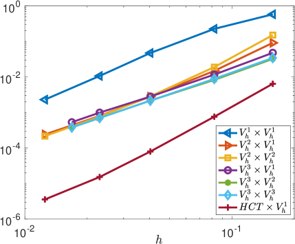
Figure 1. (Ex1)- Relative error $\|u-u_{h}\|_{L^{2}(\mathcal{M})}/\|u\|_{L^{2}(\mathcal{M})}$ with respect to $h$ for various approximation spaces (see Table 4).

When a richer space is used to approximate the dual variable $z$ than the primal one, we observe a locking phenomenon leading to unsatisfactory results. For instance, considering the approximation $V_{h}^{1}\times V_{h}^{2}$, and the mesh size $\sharp 4$, we obtain $\|z_{h}\|_{L^{2}(H^{1}_{0})}=1.24\times 10^{-1}$ and $\|u-u_{h}\|_{L^{2}(\mathcal{M})}/\|u\|_{L^{2}(\mathcal{M})}=3.62\times 10^{-1}$ to be compare with the values $6.84\times 10^{-5}$ and $8.01\times 10^{-4}$ for the $V_{h}^{2}\times V_{h}^{1}$ approximation. This property, also observed for instance for $\gamma=1.$ and $\gamma^{\star}=10^{-3}$, seems independent of the values of $\gamma$ and $\gamma^{\star}$.

To conclude this example, we emphasize that the spacetime discretization introduced in the previous sections is very well-appropriated for mesh adaptivity. Using the $V_{h}^{2}\times V_{h}^{1}$ approximation, Figure 3-left depicts the mesh obtained after seven adaptative refinements based on the local values of gradient of the primal variable $u_{h}$. Starting with a coarse mesh composed of $288$ triangles and $166$ vertex, the final mesh is composed with $13068$ triangles and $6700$ vertices. We obtain the following values: $\|z_{h}\|_{L^{2}(H^{1}_{0})}=3.76\times 10^{-3}$; $\|u-u_{h}\|_{L^{2}(\mathcal{M})}/\|u\|_{L^{2}(\mathcal{M})}=3.54\times 10^{-2}$; $\|(u-u_{h})(0)\|_{L^{2}(0,1)}/\|u(0)\|_{L^{2}(0,1)}=2.48\times 10^{-2}$; $\|(u-u_{h})_{t}(0)\|_{H^{-1}(0,1)}=3.36\times 10^{-3}$ for a CPU time equal to $2.17$.

5.2. Example 2

For our second numerical example, we consider the observation $u_{\mathcal{O}}$ based on the initial condition $u_{0}(x)=1-|2x-1|\in H^{1}_{0}(\Omega)$, $u_{1}(x)=1_{(1/3,2/3)}(x)\in L^{2}(\Omega)$ and $T=2$, $\omega=(0.1,0.3)$, considered in [CM15a, section 5.1]. The corresponding solution $u$ belongs to $H^{1}(\mathcal{M})$ but not in $H^{2}(\mathcal{M})$ and is given by

$$\mathbf{(Ex2)}\quad\left\{\begin{aligned} &u(t,x)=\sum_{k>0}\biggl{(}a_{k}\cos(k\pi t)+\frac{b_{k}}{k\pi}\sin(k\pi t)\biggr{)}\sqrt{2}\sin(k\pi t),\\ &a_{k}=\frac{4\sqrt{2}}{\pi^{2}k^{2}}\sin(\pi k/2),\quad b_{k}=\frac{1}{\pi k}\big{(}\cos(\pi k/3)-\cos(2\pi k/3)\big{)},\quad k>0.\end{aligned}\right.$$

We define the observation $u_{\mathcal{O}}$ as the restriction over $(0.1,0.3)\times(0,2)$ of the first fifty terms in the previous sum. Tables 7, 8, 9, 10 provide the norms

$$\|u-u_{h}\|_{L^{2}(\mathcal{M})}/\|u\|_{L^{2}(\mathcal{M})},\quad\|(u-u_{h})(0,\cdot)\|_{L^{2}(0,1)},\quad\|(u-u_{h})_{t}(0,\cdot)\|_{L^{2}(0,1)}$$

with respect to $h$ for the primal variable and $\|z_{h}\|_{L^{2}(H^{1}_{0})}$ with respect to $h$ for the dual variable, obtained from the formulation (5.3) and from the formulation (3.14) with $p\in\{1,2,3\},q\in\{1,2\}$ and $q<p$ (see (3.1)). We use again the dual stabilizer (3.6) with $\gamma=10^{-3}$ and $\gamma^{\star}=1.$ and $h_{F}=h_{K}=h$.

In agreement with Theorem 2, the rate of convergence with respect to $h$ depends on the regularity of the solution $u$: concerning the primal variable $u$, we obtain the following behavior $\|u-u_{h}\|_{L^{2}(\mathcal{M})}/\|u\|_{L^{2}(\mathcal{M})}\approx\beta\times h^{\tau}$ with

(5.5) $$\beta=e^{-0.51}, \tau=1.09, (u_{h},z_{h})\in V_{h}^{1}\times V_{h}^{1},$$

$$\beta=e^{-0.87}, \tau=1.29, (u_{h},z_{h})\in V_{h}^{2}\times V_{h}^{1},$$

$$\beta=e^{-0.74}, \tau=1.55, (u_{h},z_{h})\in V_{h}^{3}\times V_{h}^{1},$$

$$\beta=e^{-1.21}, \tau=1.04, (u_{h},z_{h})\in V_{h}^{2}\times V_{h}^{2},$$

$$\beta=e^{-2.38}, \tau=0.86, (u_{h},z_{h})\in HCT\times V_{h}^{1}.$$

Since the solution to be reconstructed is only in $H^{1}(\mathcal{M})$, the $H^{2}$ approximation based on the $HCT$ composite finite element is asymptotically less accurate than the polynomial approximation $V_{h}^{p}\times V_{h}^{q}$, $p>q$. We also check that increasing the order of the space for the dual variable does not improve the accuracy. Moreover, we observe the same property as the first example with respect to the choice of the parameter $\lambda$ and $\lambda^{\star}$.

We remark that, since the solution $u$ to be reconstructed, develops singularities along characteristic lines starting from the point $x=1/2$ (due to the initial position $u_{0}$) and from the points $x=1/3,2/3$ (due to the initial velocity $u_{1}$), the adaptative refinement of the mesh mentioned in the previous subsection is of particular interest here. Using the $V_{h}^{2}\times V_{h}^{1}$ approximation, Figure 3-left depicts the mesh obtained after ten adaptative refinements based on the local values of gradient of the primal variable $u_{h}$. Starting with a coarse mesh composed of $288$ triangles and $166$ vertex, the final mesh is composed with $12118$ triangles and $6213$ vertices. We obtain the following values: $\|z_{h}\|_{L^{2}(H^{1}_{0})}=2.36\times 10^{-5}$; $\|u-u_{h}\|_{L^{2}(\mathcal{M})}/\|u\|_{L^{2}(\mathcal{M})}=1.63\times 10^{-3}$; $\|(u-u_{h})(0,\cdot)\|_{L^{2}(0,1)}/\|u(0,\cdot)\|_{L^{2}(0,1)}=9.69\times 10^{-4}$; $\|(u-u_{h})_{t}(0,\cdot)\|_{H^{-1}(0,1)}/\|u_{t}(0,\cdot)\|_{H^{-1}(0,1)}=4.29\times 10^{-1}$ for a CPU time equal to $2.54$. The final mesh clearly exhibits the singularities generated by the initial data $(u_{0},u_{1})$. On the contrary, the refinement strategy coupled with the HCT element does not permit to capture so clearly such singularities, in particular the weaker ones starting from the point $x=1/3$ and $x=2/3$ (see [CM15a, Figure 1]).

$h$	$1.57\times 10^{-1}$	$8.22\times 10^{-2}$	$4.03\times 10^{-2}$	$2.29\times 10^{-2}$	$1.25\times 10^{-2}$
(5.3) -$HCT\times V_{h}^{1}$	$6.21\times 10^{-5}$	$9.57\times 10^{-5}$	$1.42\times 10^{-4}$	$1.43\times 10^{-4}$	$1.23\times 10^{-4}$
(3.14) - $V_{h}^{1}\times V_{h}^{1}$	$1.19\times 10^{-2}$	$8.21\times 10^{-3}$	$3.22\times 10^{-3}$	$1.63\times 10^{-3}$	$8.71\times 10^{-4}$
(3.14) - $V_{h}^{2}\times V_{h}^{2}$	$4.16\times 10^{-3}$	$1.97\times 10^{-3}$	$1.00\times 10^{-3}$	$5.42\times 10^{-4}$	$2.95\times 10^{-4}$
(3.14) - $V_{h}^{2}\times V_{h}^{1}$	$6.99\times 10^{-4}$	$2.85\times 10^{-4}$	$1.29\times 10^{-4}$	$6.95\times 10^{-5}$	$3.25\times 10^{-5}$
(3.14) - $V_{h}^{3}\times V_{h}^{1}$	$4.63\times 10^{-4}$	$1.60\times 10^{-4}$	$5.40\times 10^{-5}$	$2.31\times 10^{-5}$	$1.37\times 10^{-5}$

Table 7. $\mathbf{(Ex2)}$; $\|z_{h}\|_{L^{2}(0,T;H^{1}_{0}(0,1))}$ w.r.t. $h$.

$h$	$1.57\times 10^{-1}$	$8.22\times 10^{-2}$	$4.03\times 10^{-2}$	$2.29\times 10^{-2}$	$1.25\times 10^{-2}$
(5.3) -$HCT\times V_{h}^{1}$	$1.97\times 10^{-2}$	$9.72\times 10^{-3}$	$5.59\times 10^{-3}$	$3.65\times 10^{-3}$	$2.08\times 10^{-3}$
(3.14) - $V_{h}^{1}\times V_{h}^{1}$	$7.96\times 10^{-2}$	$3.86\times 10^{-2}$	$1.79\times 10^{-2}$	$9.40\times 10^{-3}$	$5.01\times 10^{-3}$
(3.14) - $V_{h}^{2}\times V_{h}^{2}$	$4.16\times 10^{-2}$	$2.22\times 10^{-2}$	$1.06\times 10^{-2}$	$5.66\times 10^{-3}$	$2.99\times 10^{-3}$
(3.14) - $V_{h}^{2}\times V_{h}^{1}$	$3..54\times 10^{-2}$	$1.62\times 10^{-2}$	$6.94\times 10^{-3}$	$3.44\times 10^{-3}$	$1.24\times 10^{-3}$
(3.14) - $V_{h}^{3}\times V_{h}^{1}$	$2.47\times 10^{-2}$	$9.70\times 10^{-3}$	$3.83\times 10^{-3}$	$1.26\times 10^{-3}$	$4.87\times 10^{-4}$

Table 8. $\mathbf{(Ex2)}$; $\|(u-u_{h})\|_{L^{2}(\mathcal{M})}/\|u\|_{L^{2}(\mathcal{M})}$ w.r.t. $h$.

$h$	$1.57\times 10^{-1}$	$8.22\times 10^{-2}$	$4.03\times 10^{-2}$	$2.29\times 10^{-2}$	$1.25\times 10^{-2}$
(5.3) -$HCT\times V_{h}^{1}$	$1.53\times 10^{-2}$	$8.76\times 10^{-3}$	$5.06\times 10^{-3}$	$3.24\times 10^{-3}$	$1.90\times 10^{-3}$
(3.14) - $V_{h}^{1}\times V_{h}^{1}$	$6.74\times 10^{-2}$	$3.33\times 10^{-2}$	$1.52\times 10^{-2}$	$8.23\times 10^{-3}$	$4.45\times 10^{-3}$
(3.14) - $V_{h}^{2}\times V_{h}^{2}$	$3.96\times 10^{-2}$	$2.17\times 10^{-2}$	$1.03\times 10^{-2}$	$5.31\times 10^{-3}$	$2.64\times 10^{-3}$
(3.14) - $V_{h}^{2}\times V_{h}^{1}$	$3.31\times 10^{-2}$	$1.55\times 10^{-2}$	$6.45\times 10^{-3}$	$2.95\times 10^{-3}$	$1.58\times 10^{-3}$
(3.14) - $V_{h}^{3}\times V_{h}^{1}$	$2.18\times 10^{-2}$	$8.95\times 10^{-3}$	$3.29\times 10^{-3}$	$1.58\times 10^{-3}$	$1.67\times 10^{-3}$

Table 9. $\mathbf{(Ex2)}$; $\|(u-u_{h})(\cdot,0)\|_{L^{2}(0,1)}/\|u(\cdot,0)\|_{L^{2}(0,1)}$ w.r.t. $h$.

$h$	$1.57\times 10^{-1}$	$8.22\times 10^{-2}$	$4.03\times 10^{-2}$	$2.29\times 10^{-2}$	$1.25\times 10^{-2}$
(5.3) -$HCT\times V_{h}^{1}$	$9.33\times 10^{-1}$	$6.33\times 10^{-1}$	$5.44\times 10^{-1}$	$4.79\times 10^{-1}$	$4.54\times 10^{-1}$
(3.14) - $V_{h}^{1}\times V_{h}^{1}$	$8.99\times 10^{-1}$	$6.07\times 10^{-1}$	$4.98\times 10^{-1}$	$4.62\times 10^{-1}$	$4.41\times 10^{-1}$
(3.14) - $V_{h}^{2}\times V_{h}^{2}$	$4.74\times 10^{-1}$	$4.20\times 10^{-1}$	$4.41\times 10^{-1}$	$4.26\times 10^{-1}$	$4.34\times 10^{-1}$
(3.14) - $V_{h}^{2}\times V_{h}^{1}$	$4.62\times 10^{-1}$	$4.22\times 10^{-1}$	$4.41\times 10^{-1}$	$4.26\times 10^{-1}$	$4.34\times 10^{-1}$
(3.14) - $V_{h}^{3}\times V_{h}^{1}$	$5.02\times 10^{-1}$	$4.24\times 10^{-1}$	$4.44\times 10^{-1}$	$4.28\times 10^{-1}$	$4.27\times 10^{-1}$

Table 10. $\mathbf{(Ex2)}$; $\|(u-u_{h})_{t}(\cdot,0)\|_{H^{-1}(0,1)}/\|(u_{t}(\cdot,0)\|_{H^{-1}(0,1)}$ w.r.t. $h$.

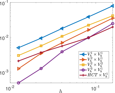
Figure 2. (Ex2)- Relative error $\|u-u_{h}\|_{L^{2}(\mathcal{M})}/\|u\|_{L^{2}(\mathcal{M})}$ with respect to $h$ for various approximation spaces (see Table 8).

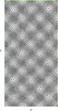
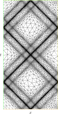
Figure 3. Locally refine spacetime meshes for the example 1 (Left) and the example 2 (Right).

6. Concluding remarks

We have introduced and analyzed a spacetime finite element approximation of a data assimilation problem for the wave equation. Based on an $H^{1}$-approximation that is nonconformal in $H^{2}$, the analysis yields error estimates for the natural norm

$$L^{\infty}(0,T;L^{2}(\Omega))\cap H^{1}(0,T;H^{-1}(\Omega))$$

of order $h^{p}$, where $p$ is the degree of the polynomials used to describe the primal variable $u$ to be reconstructed. The numerical experiments performed for two initial data, the first one in $H^{k}\times H^{k-1}$ for all $k\in\mathbb{N}$, the second one in $H^{1}\times L^{2}$, exhibit the efficiency of the method.

We emphasize that spacetime formulations are easier to implement than time-marching methods, since in particular, there is no kind of CFL condition between the time and space discretization parameters. Moreover, as shown in the numerical section, it is well-suited for mesh adaptivity.

In comparison with the formulation introduced in [CM15a], the $H^{1}$-formulation of the present work does not require the introduction of sophisticated finite element spaces. On the other hand, the formulation requires additional stabilized terms which are function of the jump of the gradient across the boundary of each element, see the definition of $s_{k}$ in (3.5). These kinds of terms are known from non-conforming approximation of fourth order problems [EGH⁺02]. So the approach can be interpreted as a non-conforming, stabilized version of the method in [CM15a]. The implementation of the stabilized terms is not straightforward in particular, in higher dimension, and is usually not available in finite element softwares. In such cases one can apply the so-called orthogonal subscale stabilization [Cod00], which can be shown to be equivalent, but requires the introduction of additional degrees of freedom, one for each component of the spacetime gradient. Another possible way to circumvent the introduction of the gradient jump terms is to consider non-conforming approximation of the Crouzeix-Raviart type as in [Bur17]. A penalty is then needed on the solution jump instead to control the $H^{1}$-conformity error. For the time discretization one could also explore the possibility of using discontinuous Petrov-Galerkin methods (see for instance [SZ18, EW19]).

The analysis performed can easily be extended to more general wave equations of the form

$$u_{tt}-div(a(x)\nabla u)+p(x,t)u=0$$

with $a\in L^{\infty}(\Omega,\mathbb{R}^{+}_{\star})$ and $p\in L^{\infty}(\mathcal{M})$ allowing to consider, through appropriate linearization techniques, data assimilation problem for nonlinear wave equation of the form $u_{tt}-\Delta u+g(u)=0$. From application viewpoint, it is also interesting to check if a spacetime approach based on a non conformal $H^{1}$-approximation can be efficient to address data assimilation problem from boundary observation. We refer to [CM15b] where a $H^{2}$ conformal approximation -similar to (5.3) - is discussed, assuming that the normal derivative $\partial_{\nu}u\in L^{2}(\Sigma)$ is available on a part large enough of $\Sigma=(0,T)\times\partial\Omega$. Eventually, the issue of the approximation of controllability problems for the wave equation through non conformal spacetime approach can very likely be addressed as well: remember that the control of minimal $L^{2}(\mathcal{O}\times(0,T))$ norm for the initial data $(z_{0},z_{1})\in H^{1}_{0}(\Omega)\times L^{2}(\Omega)$ is given by $v=u1_{\mathcal{O}}$ where $u$ together with $z$ is the saddle point of the following Lagrangian $\widehat{\mathcal{L}}:V\times L^{2}(0,T;H^{1}_{0}(\Omega))\to\mathbb{R}$

$$\widehat{\mathcal{L}}(u,z)=\frac{1}{2}\|u\|^{2}_{\mathcal{O}} +\frac{\gamma}{2}\|\Box u\|^{2}_{L^{2}(0,T;H^{-1}(\Omega))}-\int_{0}^{T}(z,\Box u)_{H_{0}^{1}(\Omega),H^{-1}(\Omega)}dt$$

$$+\langle u_{t}(\cdot,0),z_{0}\rangle_{H^{-1}(\Omega),H_{0}^{1}(\Omega)}-\langle u(\cdot,0),z_{1}\rangle_{L^{2}(\Omega)},$$

very close to (5.2). We refer to [CCM14].

References

- [AB05] Didier Auroux and Jacques Blum. Back and forth nudging algorithm for data assimilation problems. C. R. Math. Acad. Sci. Paris, 340(12):873–878, 2005.
- [AM15] Sebastián Acosta and Carlos Montalto. Multiwave imaging in an enclosure with variable wave speed. Inverse Problems, 31(6):065009, 12, 2015.
- [BFO18] Erik Burman, Ali Feizmohammadi, and Lauri Oksanen. A finite element data assimilation method for the wave equation. arXiv e-prints, page arXiv:1811.01580, Nov 2018.
- [BFO19] Erik Burman, Ali Feizmohammadi, and Lauri Oksanen. A fully discrete numerical control method for the wave equation. arXiv e-prints, page arXiv:1903.02320, Mar 2019. to appear Math. Comp.
- [BH81] Michel Bernadou and Kamal Hassan. Basis functions for general Hsieh-Clough-Tocher triangles, complete or reduced. Internat. J. Numer. Methods Engrg., 17(5):784–789, 1981.
- [BIHO18] E. Burman, J. Ish-Horowicz, and L. Oksanen. Fully discrete finite element data assimilation method for the heat equation. ESAIM Math. Model. Numer. Anal., 52(5):2065–2082, 2018.
- [BLR88] C. Bardos, G. Lebeau, and J. Rauch. Un exemple d’utilisation des notions de propagation pour le contrôle et la stabilisation de problèmes hyperboliques. Rend. Sem. Mat. Univ. Politec. Torino, (Special Issue):11–31 (1989), 1988. Nonlinear hyperbolic equations in applied sciences.
- [BLR92] Claude Bardos, Gilles Lebeau, and Jeffrey Rauch. Sharp sufficient conditions for the observation, control, and stabilization of waves from the boundary. SIAM J. Control Optim., 30(5):1024–1065, 1992.
- [BO18] E. Burman and L. Oksanen. Data assimilation for the heat equation using stabilized finite element methods. Numer. Math., 139(3):505–528, 2018.
- [BPD19] Laurent Bourgeois, Dmitry Ponomarev, and Jérémi Dardé. An inverse obstacle problem for the wave equation in a finite time domain. Inverse Probl. Imaging, 13(2):377–400, 2019.
- [BS08] S.C. Brenner and L.R. Scott. The mathematical theory of finite element methods. Springer-Verlag, third edition, 2008.
- [Bur13] Erik Burman. Stabilized finite element methods for nonsymmetric, noncoercive, and ill-posed problems. Part I: Elliptic equations. SIAM J. Sci. Comput., 35(6):A2752–A2780, 2013.
- [Bur14] Erik Burman. Error estimates for stabilized finite element methods applied to ill-posed problems. C. R. Math. Acad. Sci. Paris, 352(7-8):655–659, 2014.
- [Bur17] Erik Burman. A stabilized nonconforming finite element method for the elliptic cauchy problem. Math. Comp., pages 75–96, 2017.
- [CCM14] Carlos Castro, Nicolae Cîndea, and Arnaud Münch. Controllability of the linear one-dimensional wave equation with inner moving forces. SIAM J. Control Optim., 52(6):4027–4056, 2014.
- [CK08] Christian Clason and Michael V. Klibanov. The quasi-reversibility method for thermoacoustic tomography in a heterogeneous medium. SIAM J. Sci. Comput., 30(1):1–23, 2007/08.
- [CM15a] Nicolae Cîndea and Arnaud Münch. Inverse problems for linear hyperbolic equations using mixed formulations. Inverse Problems, 31(7):075001, 38, 2015.
- [CM15b] Nicolae Cîndea and Arnaud Münch. A mixed formulation for the direct approximation of the control of minimal -norm for linear type wave equations. Calcolo, 52(3):245–288, 2015.
- [CO16] Olga Chervova and Lauri Oksanen. Time reversal method with stabilizing boundary conditions for photoacoustic tomography. Inverse Problems, 32(12):125004, 16, 2016.
- [Cod00] Ramon Codina. Stabilization of incompressibility and convection through orthogonal sub-scales in finite element methods. Computer Methods in Applied Mechanics and Engineering, 190(13):1579 – 1599, 2000.
- [EG04] Alexandre Ern and Jean-Luc Guermond. Theory and practice of finite elements, volume 159 of Applied Mathematical Sciences. Springer-Verlag, New York, 2004.
- [EGH+02] G. Engel, K. Garikipati, T.J.R. Hughes, M.G. Larson, L. Mazzei, and R.L. Taylor. Continuous/discontinuous finite element approximations of fourth-order elliptic problems in structural and continuum mechanics with applications to thin beams and plates, and strain gradient elasticity. Computer Methods in Applied Mechanics and Engineering, 191(34):3669 – 3750, 2002.
- [EMZ16] Sylvain Ervedoza, Aurora Marica, and Enrique Zuazua. Numerical meshes ensuring uniform observability of one-dimensional waves: construction and analysis. IMA J. Numer. Anal., 36(2):503–542, 2016.
- [EW19] Johannes Ernesti and Christian Wieners. Space-time discontinuous Petrov-Galerkin methods for linear wave equations in heterogeneous media. Comput. Methods Appl. Math., 19(3):465–481, 2019.
- [EZ12] Sylvain Ervedoza and Enrique Zuazua. The wave equation: control and numerics. In Control of partial differential equations, volume 2048 of Lecture Notes in Math., pages 245–339. Springer, Heidelberg, 2012.
- [EZ13] Sylvain Ervedoza and Enrique Zuazua. Numerical approximation of exact controls for waves. SpringerBriefs in Mathematics. Springer, New York, 2013.
- [Hec12] F. Hecht. New development in Freefem++. J. Numer. Math., 20(3-4):251–265, 2012.
- [HR12] Ghislain Haine and Karim Ramdani. Reconstructing initial data using observers: error analysis of the semi-discrete and fully discrete approximations. Numer. Math., 120(2):307–343, 2012.
- [IZ99] Juan Antonio Infante and Enrique Zuazua. Boundary observability for the space semi-discretizations of the -D wave equation. M2AN Math. Model. Numer. Anal., 33(2):407–438, 1999.
- [KK08] Peter Kuchment and Leonid Kunyansky. Mathematics of thermoacoustic tomography. European J. Appl. Math., 19(2):191–224, 2008.
- [KM91] Michael V. Klibanov and Joseph Malinsky. Newton-Kantorovich method for three-dimensional potential inverse scattering problem and stability of the hyperbolic Cauchy problem with time-dependent data. Inverse Problems, 7(4):577–596, 1991.
- [KR92] Michael Klibanov and Rakesh. Numerical solution of a time-like Cauchy problem for the wave equation. Math. Methods Appl. Sci., 15(8):559–570, 1992.
- [LL67] R. Lattès and J.-L. Lions. Méthode de quasi-réversibilité et applications. Travaux et Recherches Mathématiques, No. 15. Dunod, Paris, 1967.
- [LRLTT17] Jérôme Le Rousseau, Gilles Lebeau, Peppino Terpolilli, and Emmanuel Trélat. Geometric control condition for the wave equation with a time-dependent observation domain. Anal. PDE, 10(4):983–1015, 2017.
- [Mil12] Luc Miller. Resolvent conditions for the control of unitary groups and their approximations. J. Spectr. Theory, 2(1):1–55, 2012.
- [MM19] Santiago Montaner and Arnaud Münch. Approximation of controls for linear wave equations: A first order mixed formulation. Mathematical control and related fields, 9(4):729–758, 2019.
- [Nit71] J. Nitsche. Über ein Variationsprinzip zur Lösung von Dirichlet-Problemen bei Verwendung von Teilräumen, die keinen Randbedingungen unterworfen sind. Abh. Math. Sem. Univ. Hamburg, 36:9–15, 1971. Collection of articles dedicated to Lothar Collatz on his sixtieth birthday.
- [NK16] Linh V. Nguyen and Leonid A. Kunyansky. A dissipative time reversal technique for photoacoustic tomography in a cavity. SIAM J. Imaging Sci., 9(2):748–769, 2016.
- [RTW10] Karim Ramdani, Marius Tucsnak, and George Weiss. Recovering and initial state of an infinite-dimensional system using observers. Automatica J. IFAC, 46(10):1616–1625, 2010.
- [SU09] Plamen Stefanov and Gunther Uhlmann. Thermoacoustic tomography with variable sound speed. Inverse Problems, 25(7):075011, 16, 2009.
- [SY15] Plamen Stefanov and Yang Yang. Multiwave tomography in a closed domain: averaged sharp time reversal. Inverse Problems, 31(6):065007, 23, 2015.
- [SZ90] L. R. Scott and S. Zhang. Finite element interpolation of nonsmooth functions satisfying boundary conditions. Math. Comp., 54(190):483–493, 1990.
- [SZ18] Olaf Steinnach and Marco Zank. A stabilized space-time finite element method for the wave equation. Technische Universität Graz Report 2018/5, pages 1–27, 2018.
- [Tho97] V. Thomée. Galerkin finite element methods for parabolic problems, volume 25 of Springer Series in Computational Mathematics. Springer-Verlag, Berlin, 1997.
- [Wan09] Lihong V Wang. Photoacoustic imaging and spectroscopy. CRC press, 2009.
- [Zua05] Enrique Zuazua. Propagation, observation, and control of waves approximated by finite difference methods. SIAM Rev., 47(2):197–243, 2005.