Ladder Operators in Repulsive Harmonic Oscillator with Application to the Schwinger Effect

Abstract

The ladder operators in harmonic oscillator are a well-known strong tool for various problems in physics. In the same sense, it is sometimes expected to handle the problems of repulsive harmonic oscillator in a similar way to the ladder operators in harmonic oscillators, though their analytic solutions are well known. In this paper, we discuss a simple algebraic way to introduce the ladder operators of the repulsive harmonic oscillators, which can reproduce well-known analytic solutions. Applying this formalism, we discuss the charged particles in a constant electric field in relation to the Schwinger effect; the discussion is also made on a supersymmetric extension of this formalism.

1 Introduction

The algebraic approaches to the potential problems in quantum mechanics are commonly used ways from the early state of those fields[1]. In particular, the harmonic oscillators (HOs) give a good operative example of an algebraic approach to the eigenvalue problems in terms of the ladder operators, the annihilation and creation operators $(\hat{a},\hat{a}^{\dagger})$ characterized by $[\hat{a},\hat{a}^{\dagger}]=1$. In such a dynamical system, the eigenvalue problem of Hamiltonian can be solved exactly by use of those ladder operators without depending on the representation of the eigenstates[1, 2] and, if we take the coordinate representation of those states, the eigenstates will be reduced to the well-known analytic solutions expressed in terms of Hermite polynomials. The use of ladder operators also provides necessary tools in the field theories, since the dynamical degrees of freedom of bosonic-free fields are decomposed into those of infinite harmonic oscillators.

In comparison with HOs, the physical applications of the repulsive harmonic oscillators (RHOs) are limited, since the Hamiltonian of RHOs is parabolic and its eigenstates are scattering states. The algebraic approaches to RHOs, however, have been tried from a few different viewpoints: the dynamical groups including RHOs [3, 4], the analytic continuation of angular velocity $\omega\rightarrow\pm i\omega$ in HOs[5, 6, 7], the Bose systems in SUSY quantum mechanics[8, 9], and so on.

On the other hand, it is known that the eigenvalue problems of the RHO Hamiltonian are reduced to solve Weber’s equation, which has analytic solutions so-called parabolic cylinder functions or the Weber functions[10, 11]. The relation between the algebraic approaches to RHOs and the analytic solutions, however, is not always clear. It is also important to study the completeness of the states constructed out of the algebraic approaches, since the trace calculations in physical applications require such a property of those states. The purpose of this paper is, thus, to give a simple algebraic approach to the eigenvalue problems of RHOs by introducing Hermitian ladder operators $(A,\bar{A})$ characterized by $[A,\bar{A}]=i$.

We can show that the dynamical variables of RHOs can be represented in the functional spaces constructed out of $(A,\bar{A})$ with two cyclic states $(\phi_{0},\bar{\phi}_{0})$ satisfying $A\phi_{0}=\bar{A}\bar{\phi}_{0}=0$[12]. Here, the $\{\bar{A}^{n}{\phi}_{0}\}$ and $\{A^{n}\bar{\phi}_{0}\}\,(n\in\mathbb{N})$ are conjugate, complex conjugate in the $x$-representation, states which form orthonormal pairs, though those themselves are not square integrable. Those pairs become complex conjyugate of each other in $x$ representation. As the result, those states form a discrete basis of a space of functionals $\bm{\Phi}^{\times}$, which includes the Hilbert space $\mathcal{H}$ for the RHO. It is also shown that there exist continuous bases $\{\phi_{\sigma},\bar{\phi}_{\sigma}\}\,(\sigma\in\mathbb{R})$ in $\bm{\Phi}^{\times}$, which are respective eigenstates of $A$ and $\bar{A}$.

In the next section, we study those continuous and discrete bases given in terms of the ladder operators with their cyclic states. In that place, the completeness of those bases is discussed carefully. The discussions are also made on the eigenvalue problems of the RHO Hamiltonian by considering the relation between the ladder operator formalism and the well-known analytic solutions.

In Sec. III, we discuss the applications of the present ladder operator formalism to two topics: one is a problem of charged particles under a constant electric field, the problem of the Schwinger effect[13]. This dynamical system is equivalent to RHO and the discrete basis in the ladder operator formalism is shown to be useful to evaluate that effect. As another topic, we study an extension of RHOs to a model of supersymmetry (SUSY) quantum mechanics by taking the advantage of the ladder operator formalism, though such an extension has been discussed from the early stages of RHOs. We focus our attention on the fact that the Schwinger effect for fermions is closely related to such an extended model.

Section IV is devoted to the summary of our results. In the Appendices, some mathematical problems used in the text are discussed: the analytic solutions of Hamiltonian eigenstates, a proof of completeness, and the evaluation of the Schwinger effect for fermions.

2 Ladder operators in repulsive harmonic oscillators

2.1 Summary of standard harmonic oscillators

To begin with, we summarize the ladder operator approach to the problems of the usual harmonic oscillator, to which the Hamiltonian operator of a mass $m$ particle with the characteristic frequency $\omega$ of the oscillation in one-dimensional space is given by

$$\hat{H} \!=\!\frac{1}{2m}\hat{p}^{2}+\frac{m\omega^{2}}{2}\hat{x}^{2}\!=\!\frac{\hbar\omega}{2}\left(\hat{a}^{\dagger}\hat{a}+\hat{a}\hat{a}^{\dagger}\right)\!=\!\hbar\omega\left(\hat{N}+\frac{1}{2}\right),$$ (2.1)

where $\hat{N}=\hat{a}^{\dagger}\hat{a}$ and

$$\begin{split}\hat{a}&=\sqrt{\frac{m\omega}{2\hbar}}\hat{x}+\frac{i}{\sqrt{2m\hbar\omega}}\hat{p}\,,\\ \hat{a}^{\dagger}&=\sqrt{\frac{m\omega}{2\hbar}}\hat{x}-\frac{i}{\sqrt{2m\hbar\omega}}\hat{p}\,.\end{split}$$ (2.2)

By definition $\langle\Phi|\hat{N}|\Phi\rangle=\|\hat{a}\Phi\|^{2}\geq 0$; then, because of $[\hat{a},\hat{a}^{\dagger}]=1$, one can verify that $[\hat{H},\hat{a}^{\dagger}]=\hbar\omega\hat{a}^{\dagger},\,[\hat{H},\hat{a}]=-\hbar\omega\hat{a}$, and $\|\hat{H}\Phi\|\geq\frac{\hbar\omega}{2}$ on a state $\Phi$ normalized so that $\|\Phi\|^{2}=1$ . This means that starting from the ground state $\Phi_{0}$ defined by $\hat{a}\Phi_{0}=0$ with $\|\Phi_{0}\|^{2}=1$, the states

$$\Phi_{n}=\frac{1}{\sqrt{n!}}\hat{a}^{{\dagger}n}\Phi_{0}~{}~{}~{}(n=0,1,2,3,\cdots)$$ (2.3)

satisfy the eigenvalue equations

$$\hat{H}\Phi_{n}=\hbar\omega\left(n+\frac{1}{2}\right)\Phi_{n}~{}~{}~{}(n=0,1,2,3,\cdots),$$ (2.4)

and the normalization $\langle\Phi_{n}|\Phi_{m}\rangle=\delta_{n,m}$. The importance is that the states $\{\Phi_{n}\}$ really form a complete basis of the functional space $V$, in which the canonical operators $(\hat{x},\hat{p})$ are represented. Namely, in terms of the bra and the ket states, the operator

$$\hat{I}=\sum_{n=0}^{\infty}|\Phi_{n}\rangle\langle\Phi_{n}|$$ (2.5)

is the unit operator in the functional space $V$ and one can verify

$$\langle x|\hat{I}|x^{\prime}\rangle=\delta(x-x^{\prime}),$$ (2.6)

where $\{|x\rangle\}$ are the eigenstates of $\hat{x}$ characterized by $\hat{x}|x\rangle=x|x\rangle$ and $\langle x|x^{\prime}\rangle=\delta(x-x^{\prime}),\,(x,x^{\prime}\in R)$. Furthermore, if it is necessary, the $x$ representation of $\Phi_{n}$ can be written explicitly in terms of the Hermitian polynomial $H_{n}(x)$ so that $\Phi_{n}(x)=\langle x|\Phi_{n}\rangle=\sqrt{\frac{1}{2^{n}n!}\sqrt{\frac{m\omega}{\pi\hbar}}}e^{-m\omega x^{2}/2\hbar}H_{n}(x\sqrt{m\omega/\hbar})$.

2.2 The case of repulsive harmonic oscillators

Now, for a repulsive harmonic oscillator, the Hamiltonian operator $\hat{H}_{r}$ is given from $\hat{H}$ in Eq.(2.1) by changing the sign of $\frac{m\omega^{2}}{2}\hat{x}^{2}$ ; and, a complete basis in the same functional space $V_{r}$ by means of new ladder operators can be constructed in roughly parallel with Eqs.(2.1)-(2.6). Namely, one can start with the expression

$$\hat{H}_{r} =\frac{1}{2m}\hat{p}^{2}-\frac{m\omega^{2}}{2}\hat{x}^{2}=-\frac{\hbar\omega}{2}\left(\bar{A}A+A\bar{A}\right),$$ (2.7)

where

$$\begin{split}A&=\sqrt{\frac{m\omega}{2\hbar}}\hat{x}-\frac{1}{\sqrt{2m\hbar\omega}}\hat{p}\,,\\ \bar{A}&=\sqrt{\frac{m\omega}{2\hbar}}\hat{x}+\frac{1}{\sqrt{2m\hbar\omega}}\hat{p}\,.\end{split}$$ (2.8)

By definition, $A$ and $\bar{A}\,(\neq A^{\dagger})$ are Hermitian operators themselves; however, they satisfy a similar algebra as that of $(\hat{a},\hat{a}^{\dagger})$ such as $[A,\bar{A}]=-[\bar{A},A]=i$. Further, in terms of $(A,\bar{A})$, the Hamiltonian operator $\hat{H}_{r}$ can be written as

$$\hat{H}_{r} =-i\hbar\omega\left(\Lambda+\frac{1}{2}\right)=-i\hbar\omega\left(\bar{\Lambda}-\frac{1}{2}\right),$$ (2.9)

where

$$\Lambda =-i\bar{A}A\,~{}~{}~{}\mbox{and}~{}~{}~{}\bar{\Lambda}=-iA\bar{A}~{}(\,=\Lambda+1\,)\,.$$ (2.10)

Since $\Lambda^{\dagger}=-\Lambda-1\,(\bar{\Lambda}^{\dagger}=-\bar{\Lambda}+1)$, the Hermiticity of the operator $\hat{H}_{r}$ given in Eq.(2.9) is formally guaranteed. The eigenvalue problem of $\hat{H}_{r}$ is, thus, reduced to those of the operators $\Lambda$ and $\bar{\Lambda}\,(\neq\Lambda^{\dagger})$, which are commutable with each other.

In order to solve the eigenvalue problem of $\Lambda$ and $\bar{\Lambda}$, let us introduce eigenstates $(\phi_{\sigma},\bar{\phi}_{\sigma})$ defined by

$$A\phi_{\sigma} =\left(\sqrt{\frac{m\omega}{2\hbar}}\hat{x}-\frac{1}{\sqrt{2m\hbar\omega}}\hat{p}\right)\phi_{\sigma}=\sigma\phi_{\sigma},$$ (2.11)

$$\bar{A}\bar{\phi}_{\sigma} =\left(\sqrt{\frac{m\omega}{2\hbar}}\hat{x}+\frac{1}{\sqrt{2m\hbar\omega}}\hat{p}\right)\bar{\phi}_{\sigma}=\sigma\bar{\phi}_{\sigma},$$ (2.12)

where the $\sigma$ is a real parameter. Then, the particular states $(\phi_{0},\bar{\phi}_{0})$ defined by $A\phi_{0}=\bar{A}\bar{\phi}_{0}=0$ should be regarded as the counterparts of $\Phi_{0}$ in the HO. It should be noticed that in spite of the similarity of Eq.(2.11) to the coherent state equation in the HO, the index $\sigma$ of $\phi_{\sigma}$ runs over the real continuous spectrum due to the Hermiticity of $A$ and the same is true for $\bar{\phi}_{\sigma}$.

In the $x$ representation,Eqs.(2.11) and (2.12) can be solved explicitly, and we obtain

$$\phi_{\sigma}(x) =\sqrt[4]{\frac{m\omega}{2\hbar\pi^{2}}}e^{i\frac{m\omega}{2\hbar}x^{2}-i\sqrt{\frac{2m\omega}{\hbar}}\sigma x},$$ (2.13)

$$\bar{\phi}_{\sigma}(x) =\sqrt[4]{\frac{m\omega}{2\hbar\pi^{2}}}e^{-i\frac{m\omega}{2\hbar}x^{2}+i\sqrt{\frac{2m\omega}{\hbar}}\sigma x},$$ (2.14)

where the normalizations of those states are $\langle\phi_{\sigma}|\phi_{\sigma^{\prime}}\rangle=\langle\bar{\phi}_{\sigma}|\bar{\phi}_{\sigma^{\prime}}\rangle=\delta(\sigma-\sigma^{\prime})$. In this $x$ representation, because of $\bar{\phi}_{\sigma}(x)=\langle x|\bar{\phi}_{\sigma}\rangle=\phi_{\sigma}(x)^{*}=\langle x|\phi_{\sigma}^{*}\rangle$, the bar becomes simply complex conjugation, and the functional space of $\{\phi_{\sigma}\}$ coincides with that of $\{\bar{\phi}_{\sigma}\}$ in the aggregate, though $\phi_{\sigma}$ and $\bar{\phi}_{\sigma}$ are independent states. Further, one can find the completeness of $(\phi_{\sigma},\bar{\phi}_{\sigma})$ in the form

$$\int d\sigma\langle x|\phi_{\sigma}\rangle\langle\phi_{\sigma}|x^{\prime}\rangle=\int d\sigma\langle x|\bar{\phi}_{\sigma}\rangle\langle\bar{\phi}_{\sigma}|x^{\prime}\rangle=\delta(x-x^{\prime}).$$ (2.15)

Thus, the states $\{\phi_{\sigma}\}$ and their conjugate $\{\bar{\phi}_{\sigma}\}$ are continuous complete bases of the functional space $\bm{\Phi}^{\times}$, which includes the Hilbert space $\mathcal{H}$ for the RHO in the framework of the Rigged Hilbert space.

In those continuous complete bases $\{\phi_{\sigma}\}$ and $\{\bar{\phi}_{\sigma}\}$, the aspect of the states $(\phi_{0},\bar{\phi}_{0})\in\bm{\Phi}^{\times}$satisfying $A\phi_{0}=\bar{A}\bar{\phi}_{0}=0$ are characteristic. First, the $(\phi_{0},\bar{\phi}_{0})$ should be regarded as the counterparts of the ground state $\Phi_{0}$ in the HO. Second, those states become cyclic states of $\bm{\Phi}^{\times}$ in the following sense: Writing $(\phi_{(0)},\bar{\phi}_{(0)})=(\phi_{0},\bar{\phi}_{0})$, one can verify that the states defined by

$$\phi_{(n)}=\bar{A}^{n}\phi_{(0)}~{}~{}\left(\,\bar{\phi}_{(n)}=A^{n}\bar{\phi}_{(0)}\,\right)\,,~{}(n=0,1,2,\cdots)$$ (2.16)

satisfy the eigenvalue equations

$$\Lambda\phi_{(n)}=n\phi_{(n)}~{}~{}\left(\,\bar{\Lambda}\bar{\phi}_{(n)}=-n\bar{\phi}_{(n)}\,\right)\,,~{}(n=0,1,2,\cdots).$$ (2.17)

Namely, on the states $(\phi_{(n)},\bar{\phi}_{(n)})$, the Hamiltonian operator $\hat{H}_{r}$ takes discrete eigenvalues (Fig. 1) such that

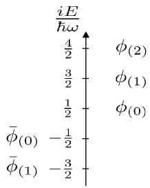
Figure 1: There are many types of complete bases in the representation space of $\hat{H}_{r}$. On the discrete bases $(\phi_{(n)},\bar{\phi}_{(n)})$, the $\hat{H}_{r}$ takes the eigenvalues shown in the figure on the left of vertical axis.

$$\left.\begin{matrix}\hat{H}_{r}\phi_{(n)}=-i\hbar\omega\left(n+\frac{1}{2}\right)\phi_{(n)}\rule[-11.38109pt]{0.0pt}{0.0pt}\\ \hat{H}_{r}\bar{\phi}_{(n)}=i\hbar\omega\left(n+\frac{1}{2}\right)\bar{\phi}_{(n)}\end{matrix}\right\}\,,~{}(n=0,1,2,\cdots),$$ (2.18)

which means that there are no ground states for $\hat{H}_{r}$ as expected from its nonpositive structure.

Those $\{\phi_{(n)},\bar{\phi}_{(n)}\}$ are the generalized eigenstates belonging to $\bm{\Phi}^{\times}$ instead of the Hilbert space for the RHO. What is important is that the states $\{\phi_{(n)}\}$ and their conjugate $\{\bar{\phi}_{(n)}\}$ are orthogonal each other under the inner product, which can be determined from the algebra of $(A,\bar{A})$ and the normalization $\langle\bar{\phi}_{(0)}|\phi_{(0)}\rangle\equiv N_{0}=\sqrt{\frac{i}{2\pi}}$ only. Indeed for $m=n+l\,(l>0)$, one can verify

$$\langle\bar{\phi}_{(m)}|\phi_{(n)}\rangle =\langle\bar{\phi}_{(0)}|A^{l}A^{n}\bar{A}^{n}|\phi_{(0)}\rangle$$

$$=in\langle\bar{\phi}_{(0)}|A^{l}A^{n-1}\bar{A}^{n-1}|\phi_{(0)}\rangle$$

$$=\cdots=i^{n}n!\langle\bar{\phi}_{(0)}|A^{l}|\phi_{(0)}\rangle,$$ (2.19)

which leads to $\langle\bar{\phi}_{(m)}|\phi_{(n)}\rangle=0\,(m>n)$; the same is true for the case $m<n$. Thus, the inner products between any $m,n$ states can be written as

$$\langle\bar{\phi}_{(m)}|\phi_{(n)}\rangle=\delta_{m,n}N_{n}~{}~{}(\,N_{n}\equiv i^{n}n!N_{0}\,),$$ (2.20)

which gives the meaning of $\{\bar{\phi}_{(n)}\}$ without depending on the representation. Here, the complexity of $N_{n}$’s again implies that the $\{\phi_{(n)},\bar{\phi}_{(n)}\}$ are not bases in a Hilbert space in spite of the resemblance between those states and $\{\Phi_{n}\}$ in the HO.

Nevertheless, Eq.(2.20) suggests that the operator

$$\hat{I}_{r}\equiv\sum_{n=0}^{\infty}\frac{1}{N_{n}}|\phi_{(n)}\rangle\langle\bar{\phi}_{(n)}|$$ (2.21)

plays the role of a unit operator in $\{\phi_{(n)}\}$ space. The expectation $\hat{I}_{r}=1$, can be confirmed through the equation

$$A\hat{I}_{r} =\sum_{n=1}^{\infty}\frac{in}{N_{n}}|\phi_{(n-1)}\rangle\langle\bar{\phi}_{(n)}|=\sum_{n=0}^{\infty}\frac{i(n+1)}{N_{n+1}}|\phi_{(n)}\rangle\langle\bar{\phi}_{(n+1)}|$$

$$=\sum_{n=0}^{\infty}\frac{1}{N_{n}}|\phi_{(n)}\rangle\langle\bar{\phi}_{(n)}|A=\hat{I}_{r}A,$$ (2.22)

which can be verified using $\frac{i(n+1)}{N_{n+1}}=\frac{1}{N_{n}}$. In a similar way, one can derive $\bar{A}\hat{I}_{r}=\hat{I}_{r}\bar{A}$. Since $A$ and $\bar{A}$ are composing elements of dynamical variables in RHOs, one can say $\hat{I}_{r}=c1,\,(c=\mbox{const})$ in the sense of Schur’s lemma. Here, the constant in the right-hand side is necessary to be $c=1$ because of $\hat{I}_{r}|\phi_{(0)}\rangle=|\phi_{(0)}\rangle$ by Eq.(2.20). In Appendix B, we will show directly

$$\langle x|\hat{I}_{r}|x^{\prime}\rangle=\delta(x-x^{\prime}),$$ (2.23)

which says that the imaginary parts of each term in the right-hand side of Eq.(2.23) are cancelled out by the summation with respect to $n$. Thus, by taking into account $(|\phi_{(n)}\rangle\langle\bar{\phi}_{(n)}|)^{\dagger}=|\bar{\phi}_{(n)}\rangle\langle\phi_{(n)}|$ and $1^{\dagger}=1$, Eq.(2.21) is equivalently represented as

$$\hat{I}_{r}=\sum_{n=0}^{\infty}\frac{1}{N^{*}_{n}}|\bar{\phi}_{(n)}\rangle\langle\phi_{(n)}|\,,$$ (2.24)

from which one can write the spectral decomposition of $\hat{H}_{r}$ so that

$$\hat{H}_{r} =\sum_{n=0}^{\infty}\frac{-i\hbar\omega\left(n+\frac{1}{2}\right)}{N_{n}}|\phi_{(n)}\rangle\langle\bar{\phi}_{(n)}|$$ (2.25)

$$=\sum_{n=0}^{\infty}\frac{i\hbar\omega\left(n+\frac{1}{2}\right)}{N^{*}_{n}}|\bar{\phi}_{(n)}\rangle\langle\phi_{(n)}|\,.$$ (2.26)

The resultant equations, (2.24)-(2.26), also have the meaning independent of the representation equation (2.21). Since $\hat{H}_{r}^{\dagger}=\hat{H}_{r}$, two types of spectral decomposition (2.25) and (2.26) are consistent and $(\phi_{(0)},\bar{\phi}_{(0)})$ are not ground states corresponding to any lower bounds of $\hat{H}_{r}$ but rather, to the cyclic states of $\bm{\Phi}^{\times}$.

The states $\{\phi_{(n)},\bar{\phi}_{(n)}\}$ form a discrete basis of $\bm{\Phi}^{\times}$ in pairs in addition to that those are generalized eigenstates of $\hat{H}_{r}$. The eigenstates of $\hat{H}_{r}$ are not limited to those states; we emphasize that the discrete basis $\{\phi_{(n)},\bar{\phi}_{(n)}\}$ is closely related to Weber’s functions, which are continuous eigenvalue solutions for an eigenvalue equation of $\hat{H}_{r}$, by means of the analytic continuation with respect to $n$. In order to verify this, we take notice the formula for a complex $\lambda$:

$$\bar{A}^{\lambda} =\frac{1}{\Gamma(-\lambda)}\int_{0}^{\infty}dte^{-\bar{A}t}t^{-(\lambda+1)}$$ (2.27)

$$=\frac{1}{\Gamma(-\lambda)}\int_{0}^{\infty}dtt^{-(\lambda+1)}e^{-\frac{i}{4}t^{2}}e^{-t\sqrt{\frac{m\omega}{2\hbar}}\hat{x}}e^{-t\frac{1}{\sqrt{2m\hbar\omega}}\hat{p}}.$$ (2.28)

Here, Eq.(2.27) seems to hold on the states such as $\{\bar{\phi}_{\sigma};\sigma>0\}$, on which $\bar{A}$ becomes an operator with positive eigenvalues. Applying Eq.(2.28) to $\phi_{(0)}(x)$, such a constraint will fade away in the sense of analytic continuation; and, we obtain the expression

$$\bar{A}^{\lambda}\phi_{(0)}(x) =\sqrt[4]{\frac{m\omega}{2\hbar\pi^{2}}}\frac{1}{\Gamma(-\lambda)}\int_{0}^{\infty}dt$$

$$\times t^{-(\lambda+1)}e^{-\frac{i}{4}t^{2}}e^{-t\sqrt{\frac{m\omega}{2\hbar}}x}e^{i\frac{m\omega}{2\hbar}\left(x+it\sqrt{\frac{\hbar}{2m\omega}}\right)^{2}}$$

$$=e^{\frac{i\pi}{4}\lambda}\sqrt[4]{\frac{m\omega}{2\hbar\pi^{2}}}\frac{e^{-\frac{1}{4}\left(e^{-\frac{i\pi}{4}}\sqrt{\frac{2m\omega}{\hbar}}x\right)^{2}}}{\Gamma(-\lambda)}\int_{0}^{\infty}d\bar{t}$$

$$\times\bar{t}^{-(\lambda+1)}e^{-\frac{1}{2}\bar{t}^{2}}e^{-\bar{t}\left(e^{-\frac{i\pi}{4}}\sqrt{\frac{2m\omega}{\hbar}}x\right)}$$

$$=e^{\frac{i\pi}{4}\lambda}\sqrt[4]{\frac{m\omega}{2\hbar\pi^{2}}}D_{\lambda}\left(z\right)\,,$$ (2.29)

where $\bar{t}=e^{\frac{i\pi}{4}}t$ and $z=e^{-\frac{i\pi}{4}}\sqrt{\frac{2m\omega}{\hbar}}x$. The last equality in Eq.(2.29) shows the relationship[16] between $\bar{A}^{\lambda}\phi_{(0)}(x)$ and Weber’s function $D_{\lambda}(z)$ (Appendix A). In a similar manner, one can verify that

$$A^{\rho}\bar{\phi}_{(0)}(x) =e^{-\frac{i\pi}{4}\rho}\sqrt[4]{\frac{m\omega}{2\hbar\pi^{2}}}D_{\rho}(iz),$$ (2.30)

which can be regarded as the analytic continuation of the relation $\bar{\phi}_{(n)}(x)=\phi_{(n)}^{*}(x)$ with respect to $n$. We note that if the $\lambda$ in Eq.(2.29) and the $\rho$ in Eq.(2.30) give the same eigenvalue of $\frac{i\hat{H}_{r}}{\hbar\omega}$, then $\lambda+\frac{1}{2}=-(\rho+\frac{1}{2})$ or $\rho=-(\lambda+1)$. Therefore, $D_{\lambda}(z)$ and $D_{-(\lambda+1)}(iz)$ are independent eigenstates of $\frac{i\hat{H}_{r}}{\hbar\omega}$ belonging to the same eigenvalue $\lambda+\frac{1}{2}$. This is a well-known result of discrete eigenstates in the eigenvalue problem of RHOs [10, 11]. In terms of Weber’s $D$ function, the completeness condition (2.23) can also be represented as

$$\langle x|\hat{I}_{r}|x^{\prime}\rangle =\sum_{n=0}^{\infty}\frac{1}{N_{n}}\phi_{(n)}(x)\bar{\phi}_{(n)}(x^{\prime})^{*}$$

$$=\sum_{n=0}^{\infty}\frac{i^{n}}{N_{n}}\left(\frac{m\omega}{2\hbar\pi^{2}}\right)^{\frac{1}{2}}D_{n}(z)D_{n}(iz^{\prime})^{*}.$$ (2.31)

In summary, the complete bases $\{\phi_{\sigma}(x)\}$ and $\{\bar{\phi}_{\sigma}(x)\}$ are respective eigenstates of $A$ and $\bar{A}$ belonging to continuous eigenvalues $\{\sigma\in\mathbb{R}\}$, but those are not eigenstates of $\hat{H}_{r}$. On the other hand, the eigenstates $\{\phi_{(n)}(x),\bar{\phi}_{(n)}(x)\}$ are eigenstates of $\hat{H}_{r}$ with discrete eigenvalues corresponding to the analytic continuation $\omega\rightarrow\pm i\omega$ of the eigenvalues in Eq.(2.4). The $\{\phi_{(n)}(x)\,\bar{\phi}_{(n)}(x)\}$ form a discrete basis of $\bm{\Phi}^{\times}$ in pairs. The $\{D_{\lambda}(z);\,\lambda\in\mathbb{R}\}$ are analytic solutions of an eigenvalue equation for $\hat{H}_{r}$; another aspect of $D_{\lambda}(z)$ is an analytic continuation of $\phi_{(n)}(x)$ with respect to $n$. The eigenstates $\{\phi_{(n)}(x),\bar{\phi}_{(n)}(x)\}$ and $\{D_{\lambda}(z),D_{\rho}(iz)\}$ stand on the same footing as scattering states of $\hat{H}_{r}$ unless any boundary conditions are added.

3 Topics related to the present RHO formalism

The complete bases $\{\phi_{\sigma}\}$ or $\{\phi_{(n)},\bar{\phi}_{(n)}\}$ based on ladder operator $(A,\bar{A})$ give us useful ways to handle the problems related to RHOs; in what follows, we exhibit two simple examples.

3.1 Schwinger effect

We note that the RHO is effectively realized by a particle interacting with a specific gauge field. Let us consider the scalar field $\Phi$ in four-dimensional spacetime for a mass $m$ particles under gauge fields $A^{\mu}$ satisfying

$$\left[\hat{\Pi}_{\mu}(A)\hat{\Pi}^{\mu}(A)+(mc)^{2}\right]\Phi(x)=0,$$ (3.1)

where $\hat{\Pi}^{\mu}(A)=\hat{p}^{\mu}-\frac{g}{c}A^{\mu}$ and $g=\pm|e|$. We here setup the gauge potentials in such a way that $(A_{c}^{0}(x),\bm{A}_{c}(x))=(-Ex^{1},\bm{0})\,(E=\mbox{const}>0)$, which produces the uniform electric field $E$ along the $x^{1}$ direction. Then,

$$\hat{\Pi}(A_{c})^{2}=2m\hat{H}_{01}+\hat{p}_{\perp}^{2},$$ (3.2)

where $\hat{p}_{\perp}=(\hat{p}_{2},\hat{p}_{3})$ and

$$\hat{H}_{01} =\frac{1}{2m}\hat{p}_{1}^{2}-\frac{1}{2m}\left(\frac{|e|E}{c}\right)^{2}\left(x^{1}+\frac{c}{gE}\hat{p}^{0}\right)^{2}.$$ (3.3)

Further, in terms of the canonical variables defined by the unitary transformation $U_{E}=e^{\frac{i}{\hbar}\left(\frac{c}{gE}\right)\hat{p}^{0}\hat{p}^{1}}$ so that

$$(X^{\mu}) =(U_{E}x^{\mu}U_{E}^{-1})=\left(x^{0}-\frac{c}{gE}\hat{p}^{1},x^{1}+\frac{c}{gE}\hat{p}^{0},x^{2},x^{3}\right),$$ (3.4)

$$(\hat{P}^{\mu}) =(U_{E}\hat{p}^{\mu}U_{E}^{-1})=(\hat{p}^{\mu}),$$ (3.5)

the Hamiltonian operator (3.3) can be written as

$$\hat{H}_{01}=\frac{1}{2m}\hat{P}_{1}^{2}-\frac{m\omega^{2}}{2}X_{1}^{2},$$ (3.6)

where the angular frequency is defined by $\omega=\frac{|e|E}{mc}$. This means that the $H_{01}$ is just the Hamiltonian of the RHO defined in the phase space $(X^{\mu},P^{\mu})$.

Now, the classical action of the gauge field under consideration is $S_{G}[A_{c}]=\frac{1}{2}\int d^{4}xE^{2}$ and the one loop correction due to the scalar field $\Phi$ adds the quantum effect $S_{Q}[A_{c}]=-i\hbar\log\{\det(\hat{\Pi}(A_{c})^{2}+(mc)^{2})\}^{-1}$ to $S_{G}[A_{c}]$ . The resultant effective action of gauge fields $S_{\rm eff}[A_{c}]=S_{G}[A_{c}]+S_{Q}[A_{c}]$ becomes

$$S_{\rm eff}[A_{c}] =S_{G}[A_{c}]$$

$$-i\hbar\int_{0}^{\infty}\frac{d\tau}{\tau}e^{-i\tau((mc)^{2}-i\epsilon)}\mbox{tr}\left(e^{-i\tau\hat{\Pi}[A_{c}]^{2})}\right)$$ (3.7)

disregarding unimportant additional constant. Namely, under the classical background gauge field $A_{c}^{\mu}$, the scalar QED gives rise to the transition amplitude $\langle 0_{\rm in}|0_{\rm out}\rangle\sim Ne^{\frac{i}{\hbar}S_{\rm eff}[A_{c}]}\,(|N|^{2}=1)$, which defines an unitary $S$-matrix element for a real $S_{\rm eff}[A_{c}]$. If the $S$ matrix contains pair productions, under which the state of the electric field is constant in time, then $\mbox{Im}S_{\rm eff}[A_{c}]\neq 0$ and we have $|\langle 0_{\rm in}|0_{\rm out}\rangle|^{2}\sim e^{-\frac{2}{\hbar}\mbox{Im}S_{\rm eff}[A_{c}]}\neq 1$. This ratio, the Schwinger effect, can be evaluated by calculating the “trace” in Eq.(3.7).

For this purpose, it is convenient to use $\{|X^{0}\rangle\otimes|\phi_{(n)}(X^{1})\rangle\otimes|X_{\perp}\rangle\}$ as the base states in the trace calculation. Then, by taking $1=\sum_{n=0}^{\infty}\frac{1}{N_{n}}|\phi_{(n)}\rangle\langle\bar{\phi}_{(n)}|$ and $\int dX^{1}\bar{\phi}_{(n)}(X^{1})^{*}\phi_{(n)}(X^{1})=N_{n}$ into account, we obtain

$$\frac{1}{\hbar} {\rm Im}S_{\rm eff}[A_{c}]=-{\rm Re}\int_{0}^{\infty}\frac{d\tau}{\tau}e^{-i\tau((mc)^{2}-i\epsilon)}$$

$$\times\mbox{tr}\left(e^{-i\tau\left(2m\hat{H}_{01}+\hat{P}_{\perp}^{2}\right)}\right)$$

$$=-{\rm Re}\int_{0}^{\infty}\frac{d\tau}{\tau}e^{-i\tau((mc)^{2}-i\epsilon)}\sum_{n=0}^{\infty}e^{-\tau 2m\hbar\omega(n+\frac{1}{2})}$$

$$\times\int dX^{0}\delta(0)\int d^{2}X_{\perp}\frac{\pi}{(2\pi\hbar)^{2}i\tau}~{}~{}\left(\,\delta(0)\sim\frac{\sqrt{m\hbar\omega}}{(2\pi\hbar)}\,\right),$$ (3.8)

where the integral in $\delta(0)=(2\pi\hbar)^{-1}\int dP^{0}$ has been cut by the typical momentum scale in the $(X^{0},X^{1})$ so that $\int dP^{0}\sim\sqrt{m\hbar\omega}$ (Appendix C). Putting here $V_{0}\sim\int dX^{0}$, $V_{\perp}\sim\int d^{2}X_{\perp}$ as cutoff volumes in $X^{0},X_{\perp}$ spaces respectively, the right-hand side of this equation becomes, with $\epsilon=+0,$

rhs $$=\delta(0)V_{0}V_{\perp}\mbox{Re}\left(\frac{i\pi}{(2\pi\hbar)^{2}}\int_{\epsilon}^{\infty}\frac{d\tau}{\tau^{2}}\frac{e^{-i\tau(mc)^{2}}}{2\sinh(\tau m\hbar\omega)}\right)$$

$$=\delta(0)V_{0}V_{\perp}\frac{i\pi(mc)^{2}}{4(2\pi\hbar)^{2}}\mbox{P}\int_{-\infty}^{\infty}\frac{dz}{z^{2}}\frac{e^{-iz}}{\sinh\left(z\frac{\hbar\omega}{mc^{2}}\right)}$$

$$=\delta(0)V_{0}V_{\perp}\frac{(m\hbar\omega)}{2(2\pi\hbar)^{2}}\sum_{n=1}^{\infty}\frac{(-1)^{n+1}}{n^{2}}e^{-\frac{n\pi c^{2}}{\hbar}\left(\frac{m^{2}c}{|e|E}\right)},$$ (3.9)

where the P denotes the principal value in the $z\,(=\tau(mc)^{2})$ integral. In terms of the momentum scale $\sqrt{m\hbar\omega}$, the volume $\int dX^{1}$ should also be given by

$$V_{1}\frac{\sqrt{m\hbar\omega}}{k\hbar}\sim 1~{}\left(V_{1}\sim\int dX^{1}\right)$$ (3.10)

with a dimensionless constant $k$. Thus, with $V_{(4)}=V_{0}V_{1}V_{\perp}$ and $\omega=m\left(\frac{|e|E}{m^{2}c}\right)$, we arrive at the expression

$$\frac{1}{\hbar}\mbox{Im}S_{\rm eff}[A_{c}]\!\sim\!\frac{1}{k}\frac{V_{(4)}m^{4}}{16\pi^{3}\hbar^{2}}\!\left(\frac{|e|E}{m^{2}c}\right)^{2}\!\sum_{n=1}^{\infty}\frac{(-1)^{n+1}}{n^{2}}e^{-\frac{n\pi c^{2}}{\hbar}\left(\frac{m^{2}c}{|e|E}\right)}.$$ (3.11)

For $k=1$, the result coincides with the formula of the pair creation given by Schwinger for scalar QED[13, 17]. It should also be noticed that one can replace the constraints on the cutoff parameters by a weaker condition $\frac{(2\pi\hbar)\delta(0)}{m\omega V_{1}}\sim\frac{1}{k}$, which allows another possible choice such as $(2\pi\hbar)\delta(0)\sim\frac{\hbar\omega}{c}$ and $V_{1}\sim\frac{k\hbar}{mc}$.

3.2 Extension to SUSY quantum mechanics

The present ladder operator formalism of RHOs is easily extended to one of SUSY quantum mechanics[18, 19, 20, 21] . To this end, let us introduce the Fermi oscillators characterized by $\{b,b^{\dagger}\}=1,\,b^{2}=b^{{\dagger}2}=0$, which can be represented in 2-dimensional vector space so that

$$b=\begin{pmatrix}0&0\\ 1&0\end{pmatrix}\,,~{}~{}~{}b^{\dagger}=\begin{pmatrix}0&1\\ 0&0\end{pmatrix}\,.$$ (3.12)

In terms of $(b,b^{\dagger})$, the supersymmetric extension of $\hat{H}_{r}$ should be

$$\hat{\mathcal{H}}_{r}=-i\hbar\omega\left(-i\bar{A}A+b^{{\dagger}}b\right)=-i\hbar\omega\begin{pmatrix}\bar{\Lambda}&0\\ 0&\Lambda\end{pmatrix}.$$ (3.13)

Then the generators of SUSY transformation defined by

$$\begin{split}Q&=-i\sqrt{\hbar\omega}Ab^{\dagger}=\sqrt{\hbar\omega}\begin{pmatrix}0&-iA\\ 0&0\end{pmatrix},\\ \bar{Q}&=-i\sqrt{\hbar\omega}\bar{A}b=\sqrt{\hbar\omega}\begin{pmatrix}0&0\\ -i\bar{A}&0\end{pmatrix}\,,\end{split}$$ (3.14)

are characterized by the algebras

$$\begin{split}[Q,A]&=\{Q,b^{\dagger}\}=0,\\ [Q,\bar{A}]&=\sqrt{\hbar\omega}b^{\dagger},~{}\{Q,b\}=-i\sqrt{\hbar\omega}A,\\ \end{split}$$ (3.15)

$$\begin{split}[\bar{Q},\bar{A}]&=\{\bar{Q},b\}=0,\\ [\bar{Q},A]&=-\sqrt{\hbar\omega}b,~{}\{\bar{Q},b^{\dagger}\}=-i\sqrt{\hbar\omega}\bar{A},\end{split}$$ (3.16)

and

$$[Q,\hat{\mathcal{H}}_{r}]=[\bar{Q},\hat{\mathcal{H}}_{r}]=0\,,~{}~{}\{Q,\bar{Q}\}=\hat{\mathcal{H}}_{r}\,.$$ (3.17)

If we introduce $Q_{1}=\frac{1}{\sqrt{2}}(\bar{Q}+Q)$ and $Q_{2}=\frac{i}{\sqrt{2}}(\bar{Q}-Q)$, the last equations can also be written as

$$\{Q_{i},Q_{j}\}=\delta_{ij}\hat{\mathcal{H}}_{r},~{}(i,j=1,2).$$ (3.18)

Those algebras should be compared with that of $N=2$ SUSY quantum mechanics, though $Q_{i}\,(i=1,2)$ are not Hermitian operators. The zero-point oscillation of $\hat{\mathcal{H}}_{r}$ is removed by this supersymmetry.

In spite of the formal resemblance of the present dynamical system to SUSY quantum mechanics of HOs, the true nature of both dynamical systems are fairly different as can be seen from $\bar{Q}\neq Q^{\dagger}$, the nonpositive structure of $\hat{\mathcal{H}}_{r}$, and so on. On the discrete complete basis $\{\phi_{(n)},\bar{\phi}_{(n)}\}$, the eigenvalue equation $\hat{\mathcal{H}}_{r}|\phi_{E}\rangle=E|\phi_{E}\rangle$ can be solved easily: for $n=1,2,\cdots$,

$$E^{+}_{n} =-i\hbar\omega n\mbox{~{}~{}doublet}$$ (3.19)

$$|\phi^{-}_{n}\rangle =\begin{pmatrix}0\\ \phi_{(n)}\end{pmatrix}=|-\rangle\otimes|\phi_{(n)}\rangle$$

$$|\phi^{+}_{n}\rangle =\frac{Q}{\sqrt{\hbar\omega n}}|\phi^{-}_{n}\rangle=\begin{pmatrix}-\frac{i}{\sqrt{n}}A\phi_{(n)}\\ 0\end{pmatrix}$$

$$E^{-}_{n} =i\hbar\omega n\mbox{~{}~{}doublet}$$ (3.20)

$$|\bar{\phi}^{+}_{n}\rangle =\begin{pmatrix}\bar{\phi}_{(n)}\\ 0\end{pmatrix}=|+\rangle\otimes|\bar{\phi}_{(n)}\rangle$$

$$|\bar{\phi}^{-}_{n}\rangle =\frac{\bar{Q}}{\sqrt{\hbar\omega n}}|\bar{\phi}^{+}_{n}\rangle=\begin{pmatrix}0\\ -\frac{i}{\sqrt{n}}\bar{A}\bar{\phi}_{(n)}\end{pmatrix},$$

where $|-\rangle=\begin{pmatrix}0\\ 1\end{pmatrix}$ and $|+\rangle=\begin{pmatrix}1\\ 0\end{pmatrix}$. Here, the mapping $|\phi^{+}_{n}\rangle=\frac{Q}{\sqrt{\hbar\omega n}}|\phi^{-}_{n}\rangle,(n\geq 1)$ can be inverted by $|\phi^{-}_{n}\rangle=i\frac{\bar{Q}}{\sqrt{\hbar\omega n}}|\phi^{+}_{n}\rangle$, and so the states $|\phi^{\pm}_{n}\rangle,\,(n=1,2,\cdots)$ form a tower of super pairs. In the same sense, the states $|\bar{\phi}^{\pm}_{n}\rangle,\,(n=1,2,\cdots)$ form another tower of super pairs .

In contrast, the states $|\phi^{-}_{0}\rangle$ and $|\bar{\phi}^{+}_{0}\rangle$ belonging to the same eigenvalue $E^{\pm}_{0}=0$ are two super singlets, which satisfy $Q_{i}|\phi^{-}_{0}\rangle=Q_{i}|\bar{\phi}^{+}_{0}\rangle=0,(i=1,2)$ . Therefore in the space of states $\{|\phi^{-}_{0}\rangle,\{|\phi^{\pm}_{n}\rangle\}\}$, the supersymmetry is realized as a good symmetry; that is, SUSY is not broken. The same is true for the space of states $\{|\bar{\phi}^{+}_{0}\rangle,\{|\bar{\phi}^{\pm}_{n}\rangle\}\}$. In each space, the operators $Q_{i}$ work as the generators of supersymmetry; however, there arises no mapping between those two spaces by $Q_{i}$ (Fig. 2).

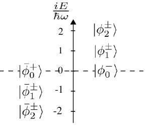
Figure 2: The eigenvalues of $\hat{\mathcal{H}}_{r}$ in an extended SUSY quantum mechanics are illustrated. The states with the superscript $\pm$ are pair states mapped by $Q$ or $\bar{Q}$. The states $|\phi^{-}_{0}\rangle$ and $|\bar{\phi}^{+}_{0}\rangle$ are fixed states under those mapping.

In the context of this SUSY quantum mechanics, we emphasize the following: in the Schwinger effect for fermions, the SUSY quantum mechanics of the RHO plays an effective role in its background; that is, topics III.A and III.B are not independent in this effect.

The Dirac field $\Psi$ interacting with an external gauge field $A^{\mu}$ obeys the $U(1)$ symmetry field equation

$$\left(\gamma\cdot\hat{\Pi}(A)+mc\right)\Psi=0~{}~{}\,\left(\,\gamma\cdot\Pi(A)=\gamma_{\mu}\Pi(A)^{\mu}\,\right).$$ (3.21)

When we multiply this equation by $-\left(\gamma\cdot\hat{\Pi}(A)-mc\right)$ from the left, the field equation becomes the second order form such that

$$\left[-\left(\gamma\cdot\hat{\Pi}(A)\right)^{2}+(mc)^{2}\right]\Psi=0.$$ (3.22)

Here, if we use the configuration of gauge potentials $(A_{c}^{0}(x),\bm{A}_{c}(x))=(-Ex^{1},\bm{0})$ as in Eq.(3.2), then with $\sigma^{\mu\nu}=\frac{i}{2}[\gamma^{\mu},\gamma^{\nu}]$ and $F_{\mu\nu}=\partial_{[\mu}(A_{c})_{\nu]}$, we obtain

$$-\left(\gamma\cdot\hat{\Pi}(A_{c})\right)^{2} =\hat{\Pi}(A_{c})^{2}-\frac{\hbar g}{2c}\sigma_{\mu\nu}F^{\mu\nu}$$

$$=\hat{\Pi}(A_{c})^{2}-\frac{\hbar g}{c}\sigma^{01}E$$

$$=2m\hat{H}_{01}+\hat{p}_{\perp}^{2}-\frac{\hbar g}{c}(i\sigma_{1}\otimes\sigma_{1})E.$$ (3.23)

Carrying out the unitary transformation in 4-spinor space by $U=e^{\frac{i\pi}{4}\sigma_{2}}\otimes e^{\frac{i\pi}{4}\sigma_{2}}$, the Eq.(3.23) becomes

$$-U \left(\gamma\cdot\hat{\Pi}(A_{c})\right)^{2}U^{\dagger}$$

$$=2m\left[-i\hbar\omega\left(-i\bar{A}A+\frac{1}{2}\right)\right]-m\hbar\omega i\sigma_{3}\otimes\sigma_{3}+\hat{p}_{\perp}^{2}$$

$$=2m\left[-i\hbar\omega\begin{pmatrix}-i\bar{A}A+b^{\dagger}b&0\\ 0&-i\bar{A}A+bb^{\dagger}\end{pmatrix}\right]+\hat{p}_{\perp}^{2},$$ (3.24)

where we have used $\sigma_{3}\otimes\sigma_{3}=\sigma_{3}\otimes[b^{\dagger},b]$ and $\omega=\frac{|e|E}{mc}$ as before. The result implies that the spectra of upper components of $\tilde{\Psi}=U\Psi$ are those of the supersymmetric Hamiltonian $\hat{\mathcal{H}}_{r}$; on the other side, the spectra of lower components of $\tilde{\Psi}$ are governed by $\hat{\mathcal{H}}^{\prime}_{r}$, which is obtained from $\hat{\mathcal{H}}_{r}$ changing the role of $(b,b^{\dagger})$. Thus, one can evaluate the Schwinger effect for fermions again according to the procedure of Eqs. (3.8) and Eq.(3.9) (Appendix D).

4 Summary

In this paper, we have discussed the eigenvalue problems of RHOs in terms of ladder operators $(A,\bar{A})$ introduced by an analogous way to the ladder operator $(\hat{a},\hat{a}^{\dagger})$ in HOs. The nonpositive property of the Hamiltonian operator $\hat{H}_{r}$ in RHOs is a result of the property of ladder operators such as $A^{\dagger}=A$, $\bar{A}^{\dagger}=\bar{A}$, and $[A,\bar{A}]=i$. Then, the eigenstates $A\phi_{\sigma}=\sigma\phi_{\sigma}$ and $\bar{A}\bar{\phi}_{\sigma}=\sigma\bar{\phi}_{\sigma}~{}(\sigma\in\mathbb{R})$ are able to normalize so that $\langle\phi_{\sigma}|\phi_{\sigma^{\prime}}\rangle=\langle\bar{\phi}_{\sigma}|\bar{\phi}_{\sigma^{\prime}}\rangle=\delta(\sigma-\sigma^{\prime})$. Namely, the $\{\phi_{\sigma},\bar{\phi}_{\sigma}\}$ are continual bases of the space of functionals $\bm{\Phi}^{\times}$ including the Hilbert space $\mathcal{H}$ of the RHO in the framework of rigged Hilbert space. Those continual bases are not eigenstates of $\hat{H}_{r}$, but rather the states related to $\{|x\rangle,\,|p\rangle\}$ by a unitary transformation.

On the other hand, the states $\phi_{(n)}=\bar{A}^{n}\phi_{(0)}$ and $\bar{\phi}_{(n)}=A^{n}\bar{\phi}_{(0)}$ $(n\in\mathbb{N})$ with $(\phi_{(0)},\bar{\phi}_{(0)})=(\phi_{0},\bar{\phi}_{0})$ are eigenstates of $\hat{H}_{r}$ belonging to the eigenvalues $\pm i\hbar\omega\left(n+\frac{1}{2}\right)$. Since those states satisfy the normalization of the form $\langle\bar{\phi}_{(m)}|\phi_{(n)}\rangle=\delta_{m,n}N_{n}$, it can be shown that the $\{\phi_{(n)},\bar{\phi}_{(n)}\}$ form a discrete complete basis of $\bm{\Phi}^{\times}$ in pairs. Contrary to this, the discrete eigenstates $\{\Phi_{n}\}$ of the Hamiltonian for a HO are the basis of a Hilbert space.

We can also show that Weber’s $D$ functions, the special functions known as analytic solutions of the eigenvalue equation for $\hat{H}_{r}$ with continuous eigenvalues, are obtained by means of the analytic continuation of $\{\phi_{(n)},\bar{\phi}_{(n)}\}$ with respect to $n$. The $D$ functions and $\{\phi_{(n)},\bar{\phi}_{(n)}\}$ stand on the same footing as the scattering states of $\hat{H}_{r}$ unless any boundary conditions are added.

As good applications of this ladder operator formalism, we have shown two topics: the Schwinger effect in scalar QED and an extension of RHO to SUSY quantum mechanics. In the first, the Hamiltonian of particles interacting with a constant electric field is shown to be canonically equivalent to one of RHOs and so the knowledge of RHOs is useful to handle the problem of pair production by the electric field. Indeed, it has been shown that the discrete complete bases $\{\phi_{(n)},\bar{\phi}_{(n)}\}$ characterized by Eq.(2.21) give a simple way to evaluate such a production rate within the framework of quantum mechanics.

Second, we have tried to extend the present RHO system to a supersymmetric dynamical system; the extended Hamiltonian $\hat{\mathcal{H}}_{r}$ is again a nonpositive Hermitian operator constructed out of fermionic oscillators $(b,b^{\dagger})$ and ladder operators $(A,\bar{A})$. The ladder operator formalism gives rise to two towers of super-pair states $|\phi^{\pm}_{n}\rangle$ and $|\bar{\phi}^{\pm}_{n}\rangle$ $(n=1,2,\cdots)$, which belong to the eigenvalues $E^{+}_{n}=-i\hbar\omega n$ and $E^{-}_{n}=i\hbar\omega n$ respectively. In addition to this, the $n=0$ states $|\phi^{-}_{0}\rangle$ and $|\bar{\phi}^{+}_{0}\rangle$ exist as two singlet states, which satisfy $Q_{i}|\phi^{-}_{0}\rangle=Q_{i}|\bar{\phi}^{+}_{0}\rangle=0,(i=1,2)$. Namely, in each space of super-pair tower states, SUSY is realized as a good symmetry, though the SUSY in this model is an extended concept from the standard one as can be seen from $Q_{i}^{\dagger}\neq Q_{i}$.

Furthermore, we have brought up the following: if we consider the Dirac fields interacting with an external electric field, then the supersymmetric structure of RHOs will be implicitly included in a loop effect of those Dirac fields. According to this line of approach, we have shown the way to evaluate the Schwinger effect for fermions in Appendix D.

The knowledge on the complete bases in RHOs under the ladder operator formalism is expected to give useful tools in various problems other than the topics discussed in this paper. For example, the Hamiltonian $\hat{\mathcal{H}}_{r}$ is able to take continuous eigenvalues on the states $(\phi_{\sigma},\bar{\phi}_{\sigma})$; in the space of those eigenstates, the SUSY may show a different feature from the standard analysis. Those are interesting future problems.

Appendix A WEBER’S FUNCTIONS AS THE ENERGY EIGENVALUE FUNCTIONS FOR THE RHO

We here summarize the standard way to make the eigenvalue functions of the RHO reduce to Weber’s functions.

In the $x$ representation with $\hat{p}=-i\hbar\frac{\partial}{\partial x}$, the eigenvalue equation of $\hat{H}_{r}$ can be written as

$$\left(-\frac{\hbar^{2}}{2m}\frac{d^{2}}{dx^{2}}-\frac{m\omega^{2}}{2}x^{2}-E\right)\psi_{E}(x)=0.$$ (A.1)

Introducing here the variable $z$ defined by

$$x=e^{\frac{i\pi}{4}}\sqrt{\frac{\hbar}{2m\omega}}z\,,~{}~{}~{}\left(\,\frac{d^{2}}{dx^{2}}=\frac{2m\omega}{i\hbar}\frac{d^{2}}{dz^{2}}\,\right),$$ (A.2)

Eq.(A.1) with $\psi_{E}(x(z))=w_{E}(z)$ gives rise to

$$-\frac{i}{\hbar\omega}\times\mbox{Eq.}(\ref{eigen-1})=\left(\frac{d^{2}}{dz^{2}}+\frac{iE}{\hbar\omega}-\frac{1}{4}z^{2}\right)w_{E}(z)=0.$$ (A.3)

Writing $\frac{iE}{\hbar\omega}=\lambda+\frac{1}{2}$ and $w_{E}(z)=w_{\lambda}(z)$, Eq.(A.3) becomes the standard form of Weber’s equation

$$\frac{d^{2}w_{\lambda}(z)}{dz^{2}}+\left(\lambda+\frac{1}{2}-\frac{z^{2}}{4}\right)w_{\lambda}(z)=0.$$ (A.4)

For $\tilde{w}_{\lambda}(z)=e^{\frac{1}{4}z^{2}}w_{\lambda}(z)$, Eq.(A.4) can also be written as

$$\left(\frac{d^{2}}{dz^{2}}-z\frac{d}{dz}+\lambda\right)\tilde{w}_{\lambda}(z)=0.$$ (A.5)

To solve Eq.(A.5), let us use the Fourier-Laplace representation

$$\tilde{w}_{\lambda}(z)=\int_{\Gamma}dte^{-zt}f_{\lambda}(t),$$ (A.6)

where $\Gamma$ is a path from $a$ to $b$ in the complex $t$ plane. Then under the integration by parts with respect to $t$, Eq.(A.5) with Eq.(A.4) gives

$$\frac{d}{dt}\big{\{}tf_{\lambda}(t)\big{\}}+\left(t+\frac{\lambda}{t}\right)\big{\{}tf_{\lambda}(t)\big{\}}=0$$ (A.7)

on the condition that $\left[e^{-zt}\left\{tf_{\lambda}(t)\right\}\right]^{b}_{a}=0$. Equation (A.7) can be solved easily so that $f_{\lambda}(t)=\mbox{const}\,e^{-\frac{1}{2}t^{2}}t^{-(\lambda+1)}$; since the boundary conditions are satisfied by $(a,b)=(0,\infty)$ for $\mbox{\rm Re}\lambda<0$ on the real $t$ axis, and we finally obtain the integral representation for $w_{\lambda}(z)=e^{-\frac{1}{4}z^{2}}\tilde{w}_{\lambda}(z)\,(=D_{\lambda}(z))$ in such a form as [16, 22]

$$D_{\lambda}(z) =\frac{e^{-\frac{1}{4}z^{2}}}{\Gamma(-\lambda)}\int_{0}^{\infty}dte^{-zt-\frac{1}{2}t^{2}}t^{-(\lambda+1)}\hskip 19.91692pt(\,\mbox{Re}\lambda<0\,)$$ (A.8)

$$=-\frac{\Gamma(\lambda+1)}{2\pi i}e^{-\frac{1}{4}z^{2}}\int_{C}dte^{-zt-\frac{1}{2}t^{2}}(-t)^{-(\lambda+1)},$$ (A.9)

where $C$ is the contour given in Fig. 3. It is not difficult to rewrite the contour integral in Eq.(A.9) to the path integral in Eq.(A.8) by taking into account $\Gamma(\lambda+1)\sin(-\pi\lambda)=\frac{\pi}{\Gamma(-\lambda)}$.

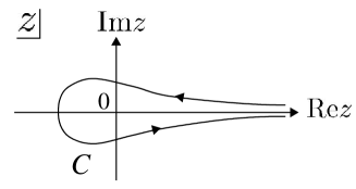
Figure 3: Contour $C$ in a complex plane

The function $D_{\lambda}(z)$ is Weber’s $D$-function (Parabolic cylinder function)[22], by which the independent solutions of Eq.(A.1) for $\frac{iE}{\hbar\omega}=\lambda+\frac{1}{2}$ are given as $D_{\lambda}(z)$ and $D_{-\lambda-1}(iz)$.

Appendix B ANOTHER PROOF OF $\hat{I}_{r}=1$.

By the definitions of $\phi_{(n)}$ and $\bar{\phi}_{(n)}$, we obtain the expression

$$\langle x|\hat{I}_{r}|x^{\prime}\rangle =\sum_{n=0}^{\infty}\frac{1}{N_{n}}\phi_{(n)}(x)\bar{\phi}_{(n)}(x^{\prime})^{*}$$

$$=\sqrt{\frac{2\pi}{i}} \sqrt{\frac{m\omega}{2\hbar\pi^{2}}}\sum_{n=0}^{\infty}\frac{1}{n!}\left(e^{-\frac{i\pi}{2}}\bar{A}A^{\prime*}\right)^{n}e^{i\frac{m\omega}{2\hbar}x^{2}}e^{i\frac{m\omega}{2\hbar}x^{\prime 2}}$$

$$=\sqrt{\frac{2\pi}{i}} \sqrt{\frac{m\omega}{2\hbar\pi^{2}}}e^{e^{-\frac{i\pi}{2}}\bar{A}A^{\prime*}}e^{i\frac{m\omega}{2\hbar}x^{2}}e^{i\frac{m\omega}{2\hbar}x^{\prime 2}}$$

$$=\sqrt{\frac{2\pi}{i}} \sqrt{\frac{m\omega}{2\hbar\pi^{2}}}e^{i\frac{m\omega}{2\hbar}x^{2}}e^{-2iA^{\prime*}\sqrt{\frac{m\omega}{2\hbar}}x}e^{\frac{i}{2}\left(A^{\prime*}\right)^{2}}e^{i\frac{m\omega}{2\hbar}x^{\prime 2}}.$$ (B.1)

Here, we have used the formula $e^{\hat{a}+\hat{b}}=e^{\hat{a}}e^{\hat{b}}e^{-\frac{1}{2}[\hat{a},\hat{b}]}$ for $[[\hat{a},\hat{b}],\hat{a}]=[[\hat{a},\hat{b}],\hat{b}]=0$, with $\hat{a}=e^{-\frac{i\pi}{2}}A^{\prime*}\sqrt{\frac{m\omega}{2\hbar}}x$ and $\hat{b}=e^{-\frac{i\pi}{2}}A^{\prime*}\frac{-1}{\sqrt{2m\hbar\omega}}\hat{p}$. Remembering, further,

$$e^{\frac{i}{2}(A^{\prime*})^{2}}=\sqrt{\frac{i}{2\pi}}\int_{-\infty}^{\infty}dke^{-\frac{i}{2}k^{2}+ikA^{\prime*}}$$ (B.2)

and using again $e^{\hat{a}+\hat{b}}=e^{\hat{a}}e^{\hat{b}}e^{-\frac{1}{2}[\hat{a},\hat{b}]}$, we arrive at

$$\langle x|\hat{I}_{r}|x^{\prime}\rangle =\sqrt{\frac{m\omega}{2\hbar\pi^{2}}}e^{i\frac{m\omega}{2\hbar}x^{2}}\int_{-\infty}^{\infty}dk$$

$$\times e^{-\frac{i}{2}k^{2}}e^{-i\left(\sqrt{\frac{2m\omega}{\hbar}}x-k\right)A^{\prime*}}e^{i\frac{m\omega}{2\hbar}x^{\prime 2}}$$

$$=\sqrt{\frac{m\omega}{2\hbar\pi^{2}}}e^{i\frac{m\omega}{2\hbar}x^{2}}\int_{-\infty}^{\infty}dk$$

$$\times e^{-\frac{i}{2}k^{2}}e^{-i\left(\sqrt{\frac{2m\omega}{\hbar}}x-k\right)\sqrt{\frac{m\omega}{2\hbar}}x^{\prime}}e^{\frac{i}{4}\left(\sqrt{\frac{2m\omega}{\hbar}}x-k\right)^{2}}$$

$$\times e^{i\frac{m\omega}{2\hbar}\left\{x^{\prime}-\left(\sqrt{\frac{2m\omega}{\hbar}}x-k\right)\sqrt{\frac{\hbar}{2m\omega}}\right\}^{2}}$$

$$=\sqrt{\frac{m\omega}{2\hbar\pi^{2}}}e^{i\frac{m\omega}{2\hbar}x^{2}}\times e^{-i\frac{2m\omega}{\hbar}xx^{\prime}+i\frac{m\omega}{\hbar}x^{2}+i\frac{m\omega}{2\hbar}x^{\prime 2}}$$

$$\times\int_{-\infty}^{\infty}dke^{ik\sqrt{\frac{2m\omega}{\hbar}}(x-x^{\prime})}=\delta(x-x^{\prime}).$$ (B.3)

Therefore, $\hat{I}_{r}$ is nothing but the unit operator for the present RHO system.

Appendix C TYPICAL MOMENTUM SCALE IN $(X^{0},X^{1})$ SPACE

The canonical pairs $(\hat{X}^{\mu},\hat{P}^{\mu}),\,(\mu=0,1)$ in Eqs. (3.4)-(3.5) can be equivalently represented by the pairs $(A,\bar{A}^{\dagger})$ and $(B,B^{\dagger})$ defined by

$$(\hat{X}^{1},\hat{P}^{1}) =\left(\sqrt{\frac{\hbar}{2m\omega}}(\bar{A}-A),\sqrt{\frac{m\hbar\omega}{2}}(\bar{A}-A)\right)$$ (C.1)

$$(\hat{X}^{0},\hat{P}^{0}) =\left(\sqrt{\frac{\hbar}{2m\omega}}(B^{\dagger}+B),i\sqrt{\frac{m\hbar\omega}{2}}(B^{\dagger}-B)\right).$$ (C.2)

Under the canonical commutation relations $[\hat{X}^{\mu},\hat{P}^{\nu}]=i\hbar\eta^{\mu\nu}$, the $(A,\bar{A}^{\dagger})$ become the ladder operators for a RHO, and the $(B,B^{\dagger})$ are oscillator variables for a HO characterized by $[B,B^{\dagger}]=1$.

In classical, the momentum square in the phase space $(X^{1},P^{1})$ can be identified with the radius square $R_{1}^{2}=2mH_{01}=-m\hbar\omega\left(\bar{A}A+A\bar{A}\right)$, where ${H}_{01}$ is the classical counterpart of the Hamiltonian (3.6). Similarly, the momentum square in the phase space $(X^{0},P^{0})$ should be given by $R_{0}^{2}=m\hbar\omega\left(B^{\dagger}B+BB^{\dagger}\right)$. In q-number theory, those radii should be evaluated by means of the expectation values through the partition functions

$$Z_{\mu}[\epsilon]={\rm Tr}e^{-i^{\delta_{1,\mu}}\epsilon\hat{R}_{\mu}^{2}}~{}~{}(\mu=0,1),$$ (C.3)

where the $\epsilon$ is a regularization parameter for those partition functions. It should be noticed that the $\hat{R}_{0}$ and the $i\hat{R}_{1}$ have real positive eigenvalues on their complete basis $\left\{|n\rangle_{B}=(n!)^{-\frac{1}{2}}B^{{\dagger}n}|0\rangle\right\}$ and $\left\{|\phi_{n}\rangle=\bar{A}^{n}|\phi_{(0)}\rangle\right\}$ with $B|0\rangle=0\,(\langle 0|0\rangle=1)$ and $A|\phi_{(0)}\rangle=\bar{A}|\bar{\phi}_{(0)}\rangle=0\,\left(\langle\bar{\phi}_{(0)}|\phi_{(0)}\rangle=\sqrt{\frac{i}{2\pi}}\right)$. Then the expectation values $\langle R^{2}_{\mu}\rangle$ can be evaluated so that

$$\langle R^{2}_{\mu}\rangle=-\frac{\partial}{\partial\epsilon}\log Z_{\mu}[\epsilon]=\hbar m\omega+\frac{2m\hbar\omega}{e^{\epsilon 2m\hbar\omega}-1}.$$ (C.4)

The first term $\hbar m\omega$ in the rightest side of Eq.(C.4) represents a typical momentum square in $(X^{0},X^{1})$ space, which is independent of the regularization.

Appendix D THE SCHWINGER EFFECT FOR FERMIONS

The action of the Dirac field $\Psi$ obeying Eq.(3.21) with the gauge fields $A_{c}^{\mu}$ is $S_{D}[\Psi,A_{c}]=\int d^{4}x\bar{\Psi}\left(\gamma\cdot\hat{\Pi}(A_{c})+mc\right)\Psi$,  $\left(\bar{\Psi}=\Psi^{\dagger}\gamma^{0}\right)$. Then the path integral result $S_{Q}[A_{c}]=-i\hbar\log\int\mathcal{D}\Psi\mathcal{D}\bar{\Psi}e^{\frac{i}{\hbar}S_{D}}=-i\hbar\mbox{Tr}\log(\gamma\cdot\hat{\Pi}+mc)+\mbox{const}$ is the quantum correction to $S_{G}[A_{c}]=\frac{1}{2}\int d^{4}xE^{2}$ so that $S_{\rm eff}[A_{c}]=S_{G}[A_{c}]+S_{Q}[A_{c}]$ becomes the effective action of $A_{c}$. Here, the “Tr”  involves the trace over four-component spinor space. To evaluate the Tr in $S_{Q}[A_{c}]$, we notice that

$$\frac{d}{da}\mbox{Tr} \log\Big{[}\gamma\cdot\hat{\Pi}+(mc)+a\Big{]}\!=\!\mbox{Tr}\frac{-(\gamma\cdot\hat{\Pi})+\{(mc)+a\}}{-(\gamma\cdot\hat{\Pi})^{2}+\{(mc)+a\}^{2}}$$

$$=\mbox{Tr}\frac{\{(mc)+a\}}{-(\gamma\cdot\hat{\Pi})^{2}+\{(mc)+a\}^{2}}$$

$$=\frac{d}{da}\left(-\frac{1}{2}\mbox{Tr}\int_{0}^{\infty}\frac{d\tau}{\tau}e^{-i\tau\left[-(\gamma\cdot\hat{\Pi})^{2}+\{(mc)+a\}^{2}-i\epsilon\right]}\right),$$ (D.1)

in consideration of which the trace of odd powers of $\gamma$ matrices vanishes. Integrating this equation with respect to $a$ from $a_{1}$ to $a_{2}$, we obtain

Tr $$\log\left[\gamma\cdot\hat{\Pi}+(mc)+a_{2}\right]-\mbox{Tr}\log\left[\gamma\cdot\hat{\Pi}+(mc)+a_{1}\right]$$

$$=-\frac{1}{2}\mbox{Tr}\int_{0}^{\infty}\frac{d\tau}{\tau}e^{i\tau\{(\gamma\cdot\hat{\Pi})^{2}+i\epsilon\}}$$

$$\times\left[e^{-i\tau\{(mc)+a_{2}\}^{2}}-e^{-i\tau\{(mc)+a_{1}\}^{2}}\right].$$ (D.2)

Setting $a_{2}=0$ and $a_{1}=-(\gamma\cdot\hat{\Pi}+mc)+1$, we get the expression

$$\mbox{Tr}\log(\gamma\cdot\hat{\Pi}+mc)=-\frac{1}{2}\mbox{Tr}\int_{0}^{\infty}\frac{d\tau}{\tau}e^{i\tau(\gamma\cdot\hat{\Pi})^{2}}e^{-i\tau\{(mc)^{2}-i\epsilon\}}$$ (D.3)

disregarding an unimportant additional constant. Then remembering Eq.(3.23) and using $e^{i\tau\frac{\hbar g}{c}E\sigma^{01}}=\cosh\left(\tau\frac{\hbar gE}{c}\right)+i\sigma^{01}\sinh\left(\tau\frac{\hbar gE}{c}\right)$, Eq.(D.3) becomes

$$\mbox{Tr}\log(\gamma\cdot\hat{\Pi} +mc)=-\frac{1}{2}\times 4\mbox{tr}\int_{0}^{\infty}\frac{d\tau}{\tau}$$

$$\times e^{-i\tau\left(\hat{\Pi}^{2}+(mc)^{2}-i\epsilon\right)}\cosh\left(\tau\frac{\hbar gE}{c}\right)$$ (D.4)

by virtue of the trace of $\sigma^{01}$ vanishes. Here, the “tr”  denotes the trace in the functional space, which yields $\mbox{tr}e^{-i\tau\hat{\Pi}^{2}}=\delta(0)V_{0}V_{\perp}\left(\frac{1}{4\pi i\hbar^{2}\tau}\right)\frac{1}{2\sinh(\tau m\hbar\omega)}$ with $\omega=\frac{|e|E}{mc}$ and $\delta(0)=\frac{\sqrt{m\hbar\omega}}{(2\pi\hbar)}$ as in the case of scalar QED. Therefore, we arrive at the expression with $\epsilon=+0$

$$\mbox{Tr}\log(\gamma\cdot\hat{\Pi}+mc) =-\delta(0)V_{0}V_{\perp}$$

$$\times\frac{2(mc)^{2}}{(2\pi\hbar)^{2}} \frac{\pi}{i}\int_{\epsilon}^{\infty}\frac{dz}{z^{2}}\frac{e^{-iz}}{\tanh\left(z\frac{\hbar\omega}{mc^{2}\pi}\right)},$$ (D.5)

where $z=\tau(mc)^{2}$. The integration with respect to $z$ in Eq.(D.5) can be carried out in the same manner as Eq.(3.9) except replacing the residue $(-1)^{n}$ of $1/\sinh(z\hbar\omega/mc^{2})$ by $1$ of $1/\tanh(z\hbar\omega/mc^{2})$. Using further $V_{1}\frac{\sqrt{m\hbar\omega}}{k\hbar}\sim 1$ with $k=1$, the resultant formula corresponding to Eq.(3.11) in the case of Dirac fields becomes

$$\frac{1}{\hbar}\mbox{Im}S_{\rm eff}[A_{c}] =-\mbox{Re}\mbox{Tr}\log\left[\gamma\cdot\hat{\Pi}(A_{c})+mc\right]$$

$$\sim V_{(4)}\frac{m^{4}}{8\pi^{3}\hbar^{2}}\left(\frac{|e|E}{m^{2}c}\right)^{2}\sum_{n=1}^{\infty}\frac{1}{n^{2}}e^{-\frac{n\pi c^{2}}{\hbar}\left(\frac{m^{2}c}{|e|E}\right)}.$$ (D.6)

This formula is nothing but the one given originally by Schwinger[13].

References

- [1] P. A. M. Dirac, The Principle of Quantum Mechanics, 4th ed. (Oxford University Press, Oxford England, 1962).
- [2] L. D. Landau and E. M. Lifshitz, Quantum Mechanics: Non-Relativistic Theory, Course of Theoretical Physics Vol.3, 3rd ed. Pergamon Press, Oxford, 1977).
- [3] E. G. Kalnins and W. Miller Jr., Lie Theory and separation of variables. 5. The equations. and , J. M. Phys. (N.Y.) 15, 1728 (1974).
- [4] C. A. Muñtoz, J. Rueda-Paz and K. B. Wolf, Discrete repulsive oscillator wave functions, J. Phys. A 42, 485210 (2009).
- [5] G. Barton, Quantum mechanics of the inverted oscillator potential, Ann. Phys. (N.Y.) 166, 322 (1986).
- [6] T. Shimbori and T. Kobayashi, Complex eigenvalues of the parabolic potential barrier and Gel’fand triplet, Nuovo Cim. B 115, 325 (2000).
- [7] K. Rajeev, S. Chakraborty and T. Padmanabhan, Inverting a normal harmonic oscillator: Physical interpretation and applications, Gen. Relativ. Gravit. 50, 116 (2018).
- [8] R. D. Mota, D. Ojeda-Guillén, M. Salazar-Ramírez, and V. D. Granados, Non-Hermitian inverted harmonic oscillator-type Hamiltonians generated from supersymmetry with reflections, Mod. Phys. Lett. A 34, 1950028 (2019).
- [9] T. Shimbori and T. Kobayashi, Supersymmetric Quantum Mechanics of Scattering, Phys. Lett. B501, 245 (2001).
- [10] E. T. Whittaker and G. N. Watson, A Course of Modern Analysis, 4th ed. (Cambridge University Press, New York, 1972), p. 347.
- [11] O. Hara and S. Naka, An example of infinite-component wave Equation without space-like solution, Prog. Theor. Phys. 53, 1194 (1975).
- [12] D. Bermudez and D. J. Fernández C, Factorization method and new potentials from the inverted oscillator, Ann. Phys. (Amsterdam) 333, 290 (2013).
- [13] J. Schwinger, On Gauge Invariance and Vacuum Polarization, Phys. Rev. 82, 664 (1951).
- [14] R. de la Madrid, The role of the rigged Hilbert space in quantum mechanics, Eur. J. Phys. 26, 287 (2005).
- [15] A. Bohm, The Rigged Hilbert Space and Quantum Mechanics, Springer Lecture Notes in Physics, Vol. 78, (Springer, Berlin, 1978).
- [16] H. Bateman, in Higher Transcendental Functions Volume II, (McGraw-Hill Book Company, Inc., New York,1953), p. 116.
- [17] G. V. Dunne, Heisenberg-Euler Effective Lagrangian: Basics and extensions, Circumnavig. Theor. Phys. 1, 445 (2005).
- [18] F. Cooper, A. Khare and U. Sukhatme, Supersymmetry in Quantum Mechanics (World Scientific Co. Pte. Ltd, Singapore, 2001).
- [19] H. Nicolai, Supersymmetry and spin systems, J. Phys. A9, 1497 (1976).
- [20] E. Witten, Dynamical breaking of supersymmetry, Nucl. Phys. B188, 513 (1981).
- [21] E. Witten, Constraints on supersymmetry breaking, Nucl. Phys. B202, 253 (1982).
- [22] Handbook of Mathematical Functions, edited by M. Abramowitz and A. Stegun (National Bureau of Standards, Washington DC, 1964), p. 689.