Rodent: Relevance determination in differential equations

Abstract

We aim to identify the generating, ordinary differential equation (ODE) from a set of trajectories of a partially observed system. Our approach does not need prescribed basis functions to learn the ODE model, but only a rich set of Neural Arithmetic Units. For maximal explainability of the learnt model, we minimise the state size of the ODE as well as the number of non-zero parameters that are needed to solve the problem. This sparsification is realized through a combination of the Variational Auto-Encoder (VAE) and Automatic Relevance Determination (ARD). We show that it is possible to learn not only one specific model for a single process, but a manifold of models representing harmonic signals as well as a manifold of Lotka-Volterra systems.

1 Introduction

Many real-world dynamical systems lack a mathematical description because it is too complicated to derive one from first principles such as symmetry or conservation laws. To tackle this problem, we introduce a novel combination of a sparsity-promoting Variational Auto-Encoder (VAE) and an ordinary differential equation (ODE) solver that can discover governing equations in the form of nonlinear ODEs. Moreover, our goal is not just to build a model for a specific ODE, but to discover the simplest mathematical formula for a manifold of ODEs parametrized by few parameters, e.g. harmonic oscillators with varying frequency $\omega$. Estimating parameters from data requires learning a mapping from the input space to a (hidden) parameter space, which makes the choice of an autoencoder natural.

Finding mathematical expressions from data is often referred to as equation discovery, a prototypical approach is called SINDy (Kaiser et al., 2018). SINDy learns a sparse selection of terms from an extensive library of basis functions, which makes it easily interpretable. But unlike us, most other approaches focus on learning a model for a single process and not for a manifold.

The rest of this section provides an informal introduction to the problem of our interest. A more formal problem definition and the description of our relevance determination in ODEs (Rodent) is given in Sec. 2 & 3.

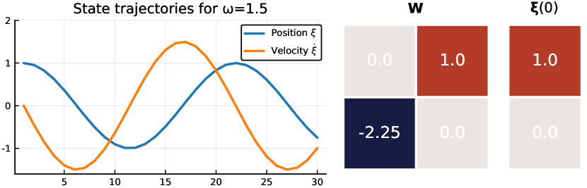
Figure 1: State trajectories of a harmonic oscillator with frequency $\omega=1.5$ on the left (position in blue, velocity in yellow). The RHS of the generating ODE (as defined in Eq. (2)) on the right.

An educating example for learning right-hand sides of ODEs is learning the manifold of harmonic oscillators. They are generated by solving the second-order ODE

$$\ddot{\xi}=-\omega^{2}\xi,$$ (1)

with position $\xi,$ acceleration $\ddot{\xi}$ (second time derivative), and frequency $\omega$ of the oscillator. Since any ODE of order $N$ can be written as a system of $N$ first order ODEs, Eq. (1) becomes

$$\frac{\partial\bm{\xi}}{\partial t}=\begin{bmatrix}\dot{\xi}\\ \ddot{\xi}\end{bmatrix} =\begin{bmatrix}0&1\\ -\omega^{2}&0\end{bmatrix}\begin{bmatrix}\xi\\ \dot{\xi}\end{bmatrix}=\bm{W}\bm{\xi},$$ (2)

with the ODE model $\bm{W}$ and the state $\bm{\xi}.$ The ODE state is composed of the oscillator’s position and its velocity. Fig. 1 shows the state trajectories of a harmonic oscillator with frequency $\omega=1.5$ and the ODE (RHS of Eq. (2)) that generates them. In practice, it is rare to observe the complete state of a dynamical system, which motivates us to learn the governing ODE from partial observations. Thus, our goal becomes to learn the RHS of Eq. (2) only by observing a set of trajectories $\{\bm{x}_{i}\}_{i=1}^{l}$ of the position $\xi$ (blue curve in Figure 1)

$$\bm{x}_{i}=[\xi_{1},\xi_{2},\ldots,\xi_{K}],$$ (3)

where each $\bm{x}_{i}$ is assumed to be generated from an oscillator with a different frequency. The downside of having access only to partial observations of $\bm{\xi}$ we cannot enforce the second state variable to be the velocity of the oscillator, i.e. the solution of the system is not unique. For example any transformation $\bm{T}=[1\;0;a\;b]$, where $a,b$ are free parameters, of Eq. (2) with transformed state $\bm{\xi}^{*}$ and transformed model $\bm{W}^{*}$

$$\bm{W}^{*} =\bm{T}\bm{W}\bm{T}^{-1} =\begin{bmatrix}-a/b&1/b\\ -\omega^{2}b-a/b&a/b\end{bmatrix}$$ (4)

$$\bm{\xi}^{*} =\bm{T}\bm{\xi} =\begin{bmatrix}\xi\\ a\xi+b\dot{\xi}\end{bmatrix}$$ (5)

is a possible solution of Eq. (2). In order to find solutions that are expected and understandable by humans, we apply automatic relevance determination (ARD; Sec. 3) to the ODE model and the state parameters.

1.1 Contributions

• Our relevant ODE identifier (Rodent) consists of a VAE with ARD prior on the latent dimension and an ODE solver as the VAE decoder, which is, to the best of our knowledge, has not been used before.

• A successfully trained Rodent is very explainable and able to output a human readable ODE:

  $$\text{explain}(\text{Rodent},[\sim]\>\text{- data})\rightarrow\ddot{\xi}=-\omega^{2}\xi+\ldots$$ (6)

  We achieve this by building the ODE model with sparse Neural Arithmetic Units (Sec. 4). We do not need a large library of predefined basis functions (as required by e.g. Kaiser et al. 2018), or prior physical knowledge (Raissi et al., 2017). We achieve sparsity by replacing the L1 regularization of the neural arithmetic units by ARD, which was shown yield better results (Wipf & Nagarajan, 2018).

• Our encoder is split into two parts: i) A dense neural network (NN) receiving the first few steps of the time-series estimates the full ODE state $\bm{\xi}$ from partial observations $\bm{x}_{i}$. ii) A convolutional NN that is agnostic to the length of the time-series learns ODE parameters $\bm{W}$.

• The system can learn not only solutions to one specific process but a manifold of solutions, e.g. to harmonic signals with a frequency parametrizing the manifold.

2 Problem definition

We are concerned with models of time-series

$$\bm{X}_{i}=[\bm{x}_{1},\bm{x}_{2},\ldots,\bm{x}_{K}]$$ (7)

with $\bm{x}_{k}\in\mathbb{R}^{d}$ that are generated by discrete-time, noisy observations of a continuous-time process

$$\bm{x}_{k}=H(\bm{\xi}(\Delta tk))+e_{k},$$ (8)

where $k=1\ldots K$ and $e_{k}\sim\mathcal{N}(0,\sigma_{e}^{2}\mathbf{I})$. The partial observation operator $H$ has fixed sampling intervals $\Delta t$, and the temporal evolution of the state variable $\bm{\xi}(t)\in\mathbb{R}^{n}$ is governed by a dynamical system described by an ODE:

$$\frac{\partial\bm{\xi}}{\partial t}= f(\bm{\theta},t).$$ (9)

The solution of the ODE for given parameters $\bm{\theta}$ and initial conditions $\bm{\xi}(0)$ is

$$\bm{\xi}(t)=\psi(\bm{\theta},\bm{\xi}(0),t),$$ (10)

where $\psi$ is a standard ODE solver, such as Tsit5 (Tsitouras, 2011). We aim to learn the structure of the ODE model from a training set of $L$ trajectories $\{\bm{X}_{i}\}_{i=1}^{L}$ generated by the same generative process but with different parameters and different initial conditions, for each trajectory, i.e.

$$\bm{X}_{i}= H(\psi(\bm{\theta}_{i},\bm{\xi}_{i}(0),\bm{t}))+\bm{e},$$ (11)

where $\bm{t}=[0,\Delta t,\ldots,K\Delta t]$. Assuming we observe a system with expected order $M$ and unknown structure, we choose $N\geq M$. Eq. (11) thus defines a generative model of sequences $\bm{X}_{i}$ from the latent space of parameters $\bm{\theta}$ and initial conditions $\bm{\xi}(0)$. Following the variational autoencoder approach (Kingma & Welling, 2013), we define the latent space $\bm{z}=[\bm{\theta},\bm{\xi}(0)]$ with the ODE (9) playing the role of the decoder. We seek an encoder in the form of a distribution $q(\bm{z}|\bm{x})$, parametrized by a deep neural network. Moreover, we use a constrictive prior $p(\bm{z})$ to promote sparsity on $\bm{z}$ to obtain a simple model, which is important for the explainability of the learnt ODEs. We will use the normal-gamma prior proposed in (Neal, 1996) and recently used e.g. in Bayesian compression of Neural Networks (Louizos et al., 2017a, b).

Our method is applicable to any differentiable dynamical system with trainable parameters $\bm{\theta}$. We will demonstrate our framework by learning parameters to Neural Arithmetic layers (Sec. 4) which aim to maximise the explainability of the learnt manifolds.

3 Rodent – Relevant ODE identifier

Figure 2: Schematic of the Rodent. Inputs and outputs in grey, latent variable $\bm{z}=[\bm{\theta},\bm{\xi}(0)]$ in the middle in brown. The encoder network $\phi_{\omega}$ on the left represents the mean of the posterior. It consists of a dense part to estimate the initial conditions and a convolutional part that is responsible for the ODE parameters. By using convolutions for the parameter estimation, we enable the network to process time-series of variable lengths. The decoder on the right is a combination of an ODE solver and the observation operator $H$. The latent variable has the ARD prior $\mathcal{N}(0,\bm{\lambda}_{z})$.

For simplicity of the notation we will write $\bm{x}=\text{vec}(\bm{X}_{i})$ for the flattened matrix of trajectories and we combine ODE state and parameters in a single latent variable $\bm{z}=[\bm{\theta},\bm{\xi}(0)]$. Further we introduce a shorthand for the ODE solver $\psi(\bm{z})=H(\psi(\bm{z},\bm{t}))$ (from Eq. (11)). Now we can define the data likelihood as

$$p(\bm{x}|\bm{z}) =\mathcal{N}(\bm{x}|\psi(\bm{z}),\sigma_{x}^{2}),$$ (12)

where the variance $\sigma_{x}^{2}$ is shared for all timesteps $\bm{t}$ and datapoints $\bm{x}$. By using an ODE solver (not a neural network) as the decoder we enforce a structure in the latent space that allows for an interpretation e.g. in terms of physical properties of the model.

To determine the structure of the ODE, we employ the Automatic Relevance Determination (ARD) prior (developed by MacKay 1994; Neal 1996) on the latent layer:

$$p(\bm{z}) =\mathcal{N}(\bm{z}|0,\text{diag}(\bm{\lambda}_{z}^{2})) p(\bm{\lambda}_{z}) =1/\bm{\lambda}_{z},$$ (13)

where a new vector variable $\bm{\lambda}_{z}>0$ of the same dimension as $\bm{z}$ has been introduced. We will treat $\bm{\lambda}_{z}$ as an unknown variable and we will seek its point estimate.

The approximated posterior distribution of the latent variable given the observed sequence is prescribed by

$$q(\bm{z}|\bm{x})=\mathcal{N}(\bm{z}|\phi_{\omega}(\bm{x}),\bm{\sigma}_{z}^{2}),$$ (14)

where mean $\bm{\mu}_{z}=\phi_{\omega}(\bm{x})$ is a deep neural network with parameters $\omega$, and both standard deviations $\bm{\lambda}_{z}$, and $\bm{\sigma_{z}}$ are shared for all datapoints $\bm{x}$. Note that we apply ARD only to the ODE parameters and initial conditions collected in $\bm{z}$ and not to the encoder network parameters $\omega$.

The parameters of the posterior are obtained by maximization of the Evidence Lower Bound (ELBO) $\mathcal{L}$:

$$\mathcal{L} =\text{E}_{p(\bm{z}|\bm{x})}\left[\log p(\bm{x}|\bm{z})\right]-\text{KL}(q(\bm{z}|\bm{x})||p(\bm{z})).$$ (15)

By applying the reparametrization trick and Monte-Carlo sampling inside the expectation we can perform stochastic gradient descent on the ELBO:

$$\mathcal{L} =\sum_{i=1}^{n}\text{E}\left[\frac{(\bm{x}_{i}-\psi(\phi_{\omega}(\bm{x}_{i})+\bm{\sigma}_{z}\odot\bm{\epsilon}))^{2}}{2\sigma_{e}^{2}}\right]+\frac{nd}{2}\log(\sigma_{e})$$ (16)

$$+\sum_{i=1}^{n}\left(\log\left(\frac{\bm{\lambda}_{z}^{2}}{\bm{\sigma_{z}}^{2}}\right)-m+\frac{\bm{\sigma_{z}}^{2}}{\bm{\lambda}_{z}^{2}}+\frac{\phi_{\omega}(\bm{x}_{i})^{2}}{\bm{\lambda}_{z}^{2}}\right),$$

with noise $\bm{\epsilon}\sim\mathcal{N}(0,I)$ and $\text{dim}(\bm{z})=m$. The ELBO is maximized with respect to the parameters $\omega$ of the encoder network, and the variances $\bm{\lambda}_{z},\bm{\sigma}_{z},\sigma_{x}$. The resulting algorithm is a relevance determination of ODEs (Rodent).

A schematic of the Rodent is shown in Fig. 2. The encoder network consists of two parts. A dense network estimating the initial state $\bm{\xi}(0)$ from the partial observations $\bm{x}$ receives only a few steps of the beginning of the time-series since this part is the most relevant for initial conditions. The second part of the encoder predicting the ODE parameters $\bm{\theta}$ is a convolutional neural net (CNN). The CNN averages over the time dimension after the convolutions, which allows it to use samples of different length.

4 Neural Arithmetic

Although it is theoretically possible to use an ODE model of arbitrary complexity (conventional NN) to represent $f(\bm{\theta},t)$, these models would be difficult to understand for humans. Therefore, we use stacks of sparse neural arithmetic units (NMU and NAU are defined below) to represent nonlinear ODEs with as few layers and parameters as possible.

Neural Multiplication Units

(NMU) as introduced by Madsen & Johansen (2020) are capable of computing products of inputs. They use explicit multiplications and a gating mechanism, which makes them easy to learn, but incapable of performing addition, subtraction, and division. We will use a Bayesian version of the NMU:

$$\hat{m}_{ij} =\max(\min(m_{ij},1),0)$$ (17)

$$a_{i} =\prod_{j}\left(x_{j}\hat{m}_{ij}+1-\hat{m}_{ij}\right),$$ (18)

where the regularisation term proposed by Madsen & Johansen (2020) is replaced by ARD acting on $m_{ij}$ (collected in a matrix $\bm{M}$).

Neural Addition Units

(NAU) can compute linear combinations (i.e. addition/subtraction). They can be easily represented by a matrix multiplication (without a bias term)

$$\bm{a}=\bm{W}\bm{x},$$ (19)

where the sparsification of $\bm{W}$ is again achieved through Bayesian compression.

An NMU layer followed by an NAU layer can thus learn additions, subtractions, and multiplications of inputs while still retaining maximal interpretability of the resulting models. Given a stack of an NMU and an NAU with input $\bm{x}=[x_{1},x_{2}]$, NMU with $\bm{M}=[1\;0;1\>1]$, and an NAU with $\bm{W}=[2,1]$ we can even write a simple macro that outputs the resulting LaTeX equation:

$$\text{NAU}(\text{NMU}(\bm{x}))=2x_{1}+x_{1}x_{2}.$$ (20)

Another interesting arithmetic unit is the Neural Arithmetic Logic Unit (NALU; Trask et al. 2018). With a slight extension it can represent addition, subtraction, multiplication, division, and arbitrary power functions. Unfortunately, the NALU suffers from unstable convergence and cannot handle negative inputs (Madsen & Johansen, 2020), which makes it infeasible for our purposes.

5 Reidentification

A perfectly trained encoder will always output good parameters that reconstruct the training sequence well. However, this task is complicated because the encoder not only has to extract the initial conditions $\bm{\xi}(0)$ from partial observations but also predict the ODE parameters $\bm{\theta}$ from a manifold of generating processes. It is likely that the encoder learns the manifold only approximately, which means that estimated parameters $\bm{z}$ are not optimal for every datapoint $\bm{x}$. Moreover, the generalization capability of the encoder outside the parameters in the training data will be limited. To solve this, we introduce another optimization step after the Rodent’s encoder is trained, which we call reidentification.

The goal of reidentification is to find the best latent code $\bm{z}$ for a given input sample $\bm{x}$ by minimizing the error of the decoder. Specifically, we minimise the reconstruction error

$$\mathcal{R}=\text{MSE}(\psi(\bm{z}),\bm{x})$$ (21)

with respect only to the relevant parameters of $\bm{z}$ (namely those with non-zero mean or variance). The loss function (21) can be easily optimized using gradient based techniques (e.g. LBFGS or SGD), as the ODE solver is differentiable, and we use samples of the latent code of the encoder $q(\bm{z}|\bm{x})$ as starting points.

As will be shown in the experimental section (in Fig. 5), reidentification helps to extrapolate far beyond the range of parameters in the training data.

6 Related work

Discovering differential equations

Learning physically relevant concepts of the two-body problem was recently solved both by Hamiltonian Neural Networks (Greydanus et al., 2019; Toth et al., 2019; Sanchez-Gonzalez et al., 2019), which learn the Hamiltonian from observations. Once the Hamiltonian is known, it is possible to derive from it most other variables of interest. While this is a very promising approach that yields good results, it is limited to systems that can be described in terms of positions and momenta such as interacting particles.
Iten et al. (2020) have shown how to discover the heliocentricity of the solar system with an autoencoder, but their architectures make significant prior assumptions, e.g. on the size of the latent space, which we do not need because we employ the ARD prior.
Similarly, Raissi et al. (2017) introduce physically informed NNs, which perform well and are very interpretable if the general structure of the problem is already known.
SINDy (Kaiser et al., 2018) is learning a few active terms from a library of basis functions, which provides a very well interpretable result, but is limited by the library of basis functions.
Another interesting approach is Koopman theory (Rudy et al., 2017; Brunton et al., 2016) which relies on finding a transformation into a higher dimensional space in which the ODE becomes linear. Combining Koopman theory and autoencoders has produced promising results, such as learning surrogates for a nonlinear pendulum and the Lorenz system (Champion et al., 2019). While the Koopman approach provides very accurate predictions once its nonlinear transformation is found, it lacks explainable results which we provide by learning the ODEs directly.

Bayesian compression

Recent work has shown that adopting a Bayesian point of view to parameter pruning can significantly reduce computational cost while still achieving competitive accuracy (Louizos et al., 2017a, b). These approaches focus on pruning network weights or complete neurons to decrease computational cost and reduce overfitting. Our approach, however, enforces sparsity only on the latent variable and the main goal is interpretability of the latent variable.

Hyper networks

are neural nets that generate weights for another network (Ha et al., 2016). Our encoder can be seen as a kind of hypernetwork, as it estimates the parameters of ODE, which can be seen as a continuous-time residual neural network (Chen et al., 2018).

7 Experiments

In this section, we demonstrate how the Rodent learns two different systems. We begin by learning a simple manifold of harmonic signals (Sec. 7.1), two superimposed harmonic signals, and then identify the equations of a nonlinear ODE called the Lotka-Volterra (LK) system (Sec. 7.3).

7.1 Identification of the harmonic oscillator

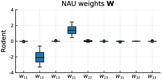
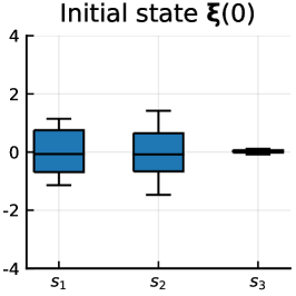
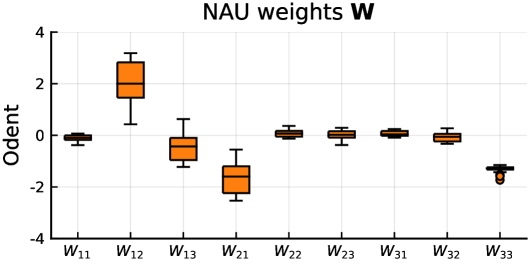
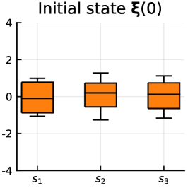
Figure 3: Comparison of the latent distributions for samples from Eq. (25) of a Rodent (with ARD) and an Odent (without ARD). The ODE model is an NAU with three units. Each box represents the distribution of one parameter of the ODE. The Rodent, which applies ARD to the latent variable clearly pushes all irrelevant parameters to zero.

An ideal identification of the harmonic oscillator would be the discovery of Eq. (2). Assuming we know that the system can be described by a linear ODE, we can represent it by a 2$\times$2-NAU layer. Thus, we want to learn an encoder that outputs both the NAU parameters $\bm{W}$, the initial position $\xi(0)$ and the velocity $\dot{\xi}(0)$ for a given trajectory of observed positions

$$\bm{x}=[\xi_{1},\ldots,\xi_{K}].$$ (22)

This means that we have six parameters of which only four are relevant: ”1”, ”$\omega^{2}$”, and the two initial conditions $\xi(0)$ and $\dot{\xi}(0)$. To demonstrate the strength of ARD, we over-parameterize the problem with a third-order ODE (equivalent to a 3$\times$3-NAU):

$$f(\bm{\theta},t)\approx\text{NAU}(\bm{\xi},t)=\bm{W}\bm{\xi}(t)$$ (23)

This third order ODE has twelve parameters in total, of which still only four are relevant. The observation operator $H$ is defined such that only the first component of the state enters into the ELBO:

$$\psi(\bm{z})=H\cdot\psi(\bm{\theta},\bm{\xi}(0),\bm{t})=[1,0,0]\cdot\psi(\bm{\theta},\bm{\xi}(0),\bm{t}).$$ (24)

To demonstrate the advantage of the ARD prior, we train a Rodent and its variant lacking the ARD prior to reconstruct harmonic signals sampled from

$$p(\bm{x}|\omega,\alpha_{0},\sigma_{e})=\mathcal{N}(\bm{x}|\sin(\omega\bm{t}+\alpha_{0}),\sigma_{e}),$$ (25)

where $p(\alpha_{0})=\mathcal{U}(0,2\pi)$ and $p(\omega)=\mathcal{U}(0.5,3)$. For both Rodent and Odent the dense part of the encoder (which predicts $\bm{\xi}(0)$) has two relu layers with 50 neurons. The convolutional part (responsible for $\bm{W}$) has three convolutional layers with 16 channels and a filter size of 3$\times$1.

The identified manifolds

of ODEs that are represented by the learnt latent distributions of Rodent and Odent are shown in Fig. 3. Both Rodent and Odent learn a reduced structure of the latent space, but we can clearly see that the pruning is much more effective in the Rodent. It keeps only four relevant parameters with the rest being almost exactly zero, while without ARD, seven parameters remain and the rest is not as close to zero. ARD penalizes large variances in its prior $\mathcal{N}(0,\bm{\lambda}_{z})$ which provides the increased pressure towards zero. The Odent has some, but less, pressure towards zero because of the fixed standard normal prior $\mathcal{N}(0,1)$.

An exemplary Rodent reconstruction and the latent mean corresponding to a harmonic signal with frequency $\omega=1.5$ is shown in Fig. 4. The latent codes resemble the desired result shown in Fig. 1. The position trajectory matches up nicely, but the second state variable does not exactly represent the velocity. Substituting variables for the four relevant parameters in Eq. (4) and Eq. (5) we can write $\bm{W}^{*}=[0\;w_{1};w_{2}\;0]$, and $\bm{\xi}^{*}=[s_{1},s_{2}]$ (where we omitted the third, irrelevant row). It follows that

$$w_{1} =1/b s_{1} =\xi$$ (26)

$$w_{2} =-\omega^{2}b s_{2} =b\dot{\xi}$$ (27)

where in the case of Fig. 4: $b=0.65$ and $\omega=1.49$, which is close to the original frequency of $\omega=1.5$. Apart from the additional degree of freedom in $b$, which comes from the partial observation of the ODE state, the Rodent successfully identified the simplest solution to the harmonic oscillator.

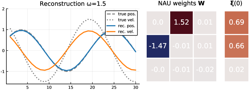
Figure 4: The left plot shows an exemplary input sequence $\bm{x}$ (dashed) and its reconstruction (blue). The reconstruction is obtained by solving the ODE defined by the parameters shown the two plots on the right. Our framework identified a sparse manifold that is very close to the desired solution shown in Eq. (2). The second state variable differs from the true velocity by a factor $b=1/1.52$, which comes from an additional degree of freedom that is introduced by the partial observation.

Extrapolation

To demonstrate that the Rodent has learnt the manifold of harmonic signals, Fig. 5 shows the reconstruction error of harmonic samples with frequencies $[2.8,3.0,\ldots,3.8,4]$, which except the frequency $2.8$ are outside frequencies used to generate training data, random Gaussian noise, and a square signal of a frequency within the trained range. Blue boxes represent the error of samples with the latent variables as proposed by the encoder. Notice that their error quickly increases as the frequency increases beyond the trained frequency range (i.e. over 3). If we reidentify the parameters, the error drops to very low values, which means that the Rodent can extrapolate far beyond its training range. Higher errors for Gaussian noise and square signals stay much higher than those of harmonic signals which indicates that these signals are outside the manifold. This means that the model of harmonic signals identified by the Rodent is correct.

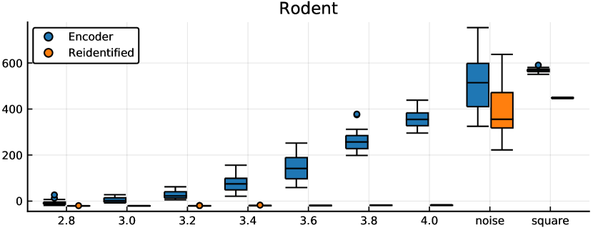
Figure 5: Reconstruction error of time-series that are generated by different models: sine waves of frequency $\omega=\{2.8,\ldots,4.0$}, (denoted by the frequency value on x-axis), square signal and Gaussian noise. Reconstruction error based on parameters from the encoder in blue, error based on reidentified parameters in yellow.

Adding the NMU

extends the capabilities of the Rodent from learning linear ODEs to nonlinear ODEs with products of state variables. For the harmonic oscillator this is of course not necessary, but just to demonstrate that ARD is powerful enough to prune the weights of the excess NMU we show it in Fig. 6. The ODE model then reads:

$$f(\bm{\theta},t)\approx\text{NAU}_{\bm{\theta}}(\text{NMU}_{\bm{\theta}}(\bm{\xi}(t)))$$ (28)

The NMU just picks out two state variables such that the hidden activation becomes $\bm{h}=[s_{2},1,s_{1}]^{\prime}$, which is then passed to the NAU with the same result as before.

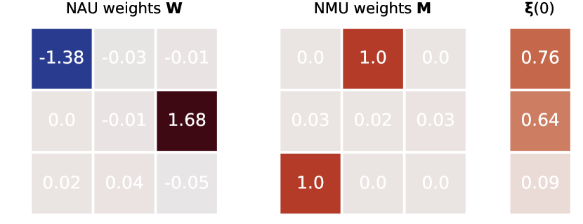
Figure 6: Latent space of the Rodent with chained NMU and NAU (Eq. (28)) that is trained to reconstruct harmonic signals. In the example the generating frequency is $\omega=2.5$.

7.2 Superimposed harmonic oscillators

The influence of different observation operators can be nicely demonstrated by letting the Rodent identify two superimposed harmonic oscillators. We sample time-series from

$$p(\bm{x}|\alpha_{0},\sigma_{e})=\mathcal{N}(\bm{x}|\sin(\omega_{1}(\bm{t}+\Delta t))+\sin(\omega_{2}(\bm{t}+\Delta t)),\sigma_{e}),$$

where $\omega_{1}=0.5$, $\omega_{2}=0.8$, and $p(\Delta t)=\mathcal{U}(0,2\pi/\omega_{1})$. Assume we want to learn a system with two oscillators with minimal observation operator that only sees the superimposed position ($H=[1,0,0,0,0]$). In this case we will need an NAU with at least four states (two for each oscillator) and another state which contains their sum. Hence we train a Rodent with a 5$\times$5-NAU, which results in a latent structure as shown in Fig. 7. A crude calculation based on the previous experiment would suggest two parameters in $\bm{W}$ for each oscillator plus two for their summation. Surprisingly the number of relevant parameters is five, so ARD found a way of removing another parameter. Further, the Rodent does learn a sum of two state variables $s_{4}$ and $s_{5}$ (row one of $\bm{W}$), but the rest of the NAU does not look like two oscillators. In fact, as we can see in Fig. 8 it seems like the Rodent learnt a superposition of one harmonic oscillator and another, more complicated trajectory. This demonstrates that the simplest solution, in terms of the number of parameters, is not always the most interpretable one. We gain no advantage from learning a superposition of a sinus and something that is essentially as complicated as the input data, although ARD reduced the number of parameters even further than expected.

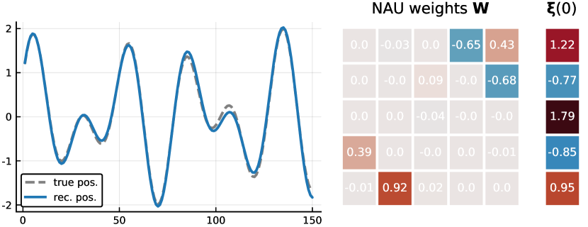
Figure 7: Rodent learning superimposed oscillators with observation operator $H=[1,0,0,0,0]$, which is too minimal to force the Rodent to learn two harmonic oscillators as basis functions. The summation of two states in the observed first state variable is just by chance.

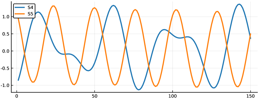
Figure 8: State trajectories of the two states that are summed by the Rodent with a 5$\times$5-NAU. One of them approximately harmonic, the other more complicated. The Rodent did not decouple the superimposed signal.

With a slightly more restrictive observation operator that sums two arbitrary state variables (here $H=[1,0,1,0]$ we can encourage the Rodent to learn a superposition of harmonic oscillators. As $H$ takes over the summation, we can also downsize the NAU to 4$\times$4. Fig. 9 shows the latent mean, which resembles two oscillators.

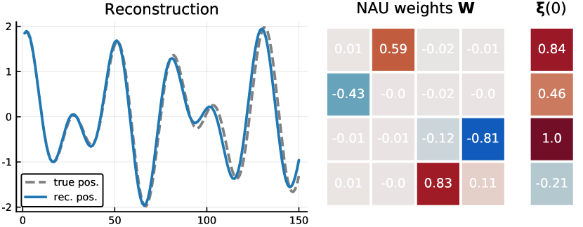
Figure 9: Rodent with 4$\times$4-NAU and $H=[1,0,0,0]$, which learns to decouple the superimposed inputs. The two decoupled oscillators are visible in the latent means on the right.

Plotting all state trajectories (Fig. 10) reveals that the Rodent now indeed learns to decouple the superimposed input signal. The two yellow lines show position (solid line) and its transformed derivative (dashed line) of the first oscillator, and the two blue lines show the same for the second oscillator. This experiment concludes that the simplicity that ARD enforces does not necessarily align with our human idea of simplicity, which favours the decomposable result.

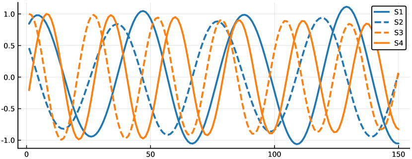
Figure 10: State trajectories of the Rodent with a 4$\times$4-NAU. The two yellow lines represent position and transformed derivative of the first oscialltor, the blue lines represent the second oscillator respectively.

7.3 Lotka-Volterra System

A system that requires the nonlinear capabilities of the Rodent is the Lotka-Volterra (LK) system:

$$\dot{x} =\alpha x-\beta xy$$ (29)

$$\dot{y} =-\delta y+\gamma xy$$ (30)

It describes the dynamical evolution of a predator population $y$ and a prey population $x$. To obtain one input sample $\bm{x}$ we solve the LK system for $N=600$ timesteps $\Delta t=0.1$ with parameters that are sampled from

$$p(\alpha) =\mathcal{U}(2,2.5) \beta=1$$ (31)

$$p(\delta) =\mathcal{U}(3,3.5) \gamma=1$$ (32)

and pick out a random starting point from within the resulting sequence. In this example, we observe the full state with the operator $H$:

$$\psi(\bm{z})=\text{vec}([1,1]\cdot\psi(\bm{\theta},\bm{\xi}(0),\bm{t})).$$ (33)

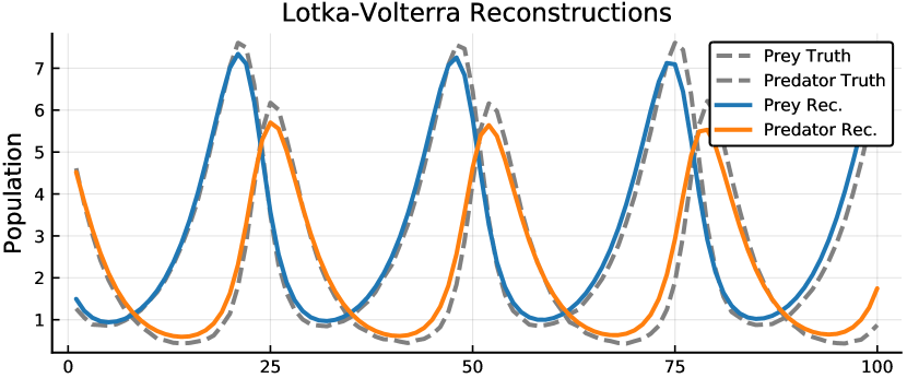
Figure 11: True evolution of the LK system compared to reconstructions created by the Rodent. Corresponding latent means in Fig. 12.

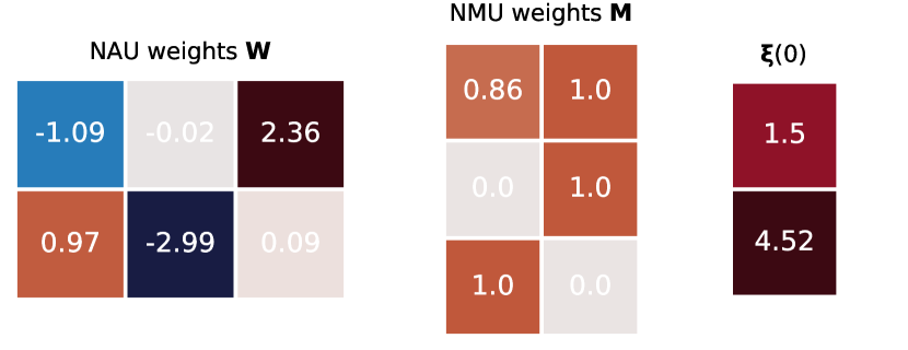
Figure 12: Latent means of an NAU/NMU chain that decodes into an LK sequence. The NMU weights can be read as a matrix multiplication where all sums are replaced by products. It performs the necessary multiplications, while the NAU weights represent the LK parameters $\alpha,\beta,\delta$, and $\gamma$. Corresponding reconstruction in Fig. 11.

Fig. 11 shows the reconstructions of the Rodent for both predator and prey populations. Fig. 12 depicts the ODE that produced the reconstruction. The NMU in the first layer of the ODE creates the necessary products ($xy,x,y$) which are then summed by the second NAU layer to produce the correct ODE. The resulting parameters are very close to the optimal solution in Eq. (29).

8 Conclusion

We have shown how to discover the governing equations of a subset of nonlinear ODEs purely from partial observations of the ODE’s state. This was done by extending the VAE with ARD and by replacing the decoder by an ODE solver, which results in the relevant ODE identifier (Rodent). Our approach results in a highly interpretable latent space containing physical meaning from which we can read out the governing equation of the analysed system. We demonstrated that it is possible to learn not only a single model for a given system, but a manifold that represents a more general class of systems. After the correct manifold is identified, it is possible to extrapolate far beyond the training range, which is another hint at the Rodent’s ability to extract physical concepts from data. Extending the VAE by ARD lead to a significant increase in the sparsity of the latent space, which is key to an interpretable result. Our approach reaches its limits as soon as the observation operator is too loose. Such an operator introduces degrees of freedom in the system that impair the Rodent’s ability to distil data into a form that is simple for humans.

A promising extension of the Rodent would be to split the ODE model into a shared and a specific part. The example of the harmonic oscillator contains variable parameters, namely $\omega$ and the initial state $\bm{\xi}(0)$, as well as a constant parameter “1”. It would be possible to learn an ODE that is fixed for all samples and let the encoder output an ODE that is specific for each sample

$$f(\bm{\theta},t)\approx g(\bm{\theta}_{\text{shared}})+h(\bm{\theta}_{\text{spec}}).$$ (34)

Another obvious extension of our model would be to increase the richness of the ODEs that can be learnt in the latent space of the Rodent. This would be possible by using the extended NALU from Sec. 4 that can learn arbitrary power functions. To do this, we would need to solve the problem of recovering the sign of the input in the multiplication layer, which might also make convergence more stable. A further extension to partial differential equations will be explored in future work.

9 Acknowledgments

Research presented in this work has been supported by the Grant Agency of the Czech Republic no. 18-21409S. The authors also acknowledge the support of the OP VVV MEYS funded project CZ.02.1.01/0.0/0.0/16_019/0000765 “Research Center for Informatics”.

References

- Brunton et al. (2016) Brunton, S. L., Proctor, J. L., and Kutz, J. N. Discovering governing equations from data by sparse identification of nonlinear dynamical systems. Proceedings of the National Academy of Sciences, 113(15):3932–3937, April 2016. ISSN 0027-8424, 1091-6490. doi: 10.1073/pnas.1517384113. URL http://www.pnas.org/lookup/doi/10.1073/pnas.1517384113.
- Champion et al. (2019) Champion, K., Lusch, B., Kutz, J. N., and Brunton, S. L. Data-driven discovery of coordinates and governing equations. pp. 27, 2019.
- Chen et al. (2018) Chen, T. Q., Rubanova, Y., Bettencourt, J., and Duvenaud, D. K. Neural ordinary differential equations. In Advances in neural information processing systems, pp. 6571–6583, 2018.
- Greydanus et al. (2019) Greydanus, S., Dzamba, M., and Yosinski, J. Hamiltonian Neural Networks. arXiv:1906.01563 [cs], September 2019. URL http://arxiv.org/abs/1906.01563. arXiv: 1906.01563.
- Ha et al. (2016) Ha, D., Dai, A., and Le, Q. V. HyperNetworks. arXiv:1609.09106 [cs], December 2016. URL http://arxiv.org/abs/1609.09106. arXiv: 1609.09106.
- Iten et al. (2020) Iten, R., Metger, T., Wilming, H., del Rio, L., and Renner, R. Discovering physical concepts with neural networks. arXiv:1807.10300 [physics, physics:quant-ph], January 2020. URL http://arxiv.org/abs/1807.10300. arXiv: 1807.10300.
- Kaiser et al. (2018) Kaiser, E., Kutz, J. N., and Brunton, S. L. Sparse identification of nonlinear dynamics for model predictive control in the low-data limit. Proceedings of the Royal Society A: Mathematical, Physical and Engineering Sciences, 474(2219):20180335, November 2018. ISSN 1364-5021, 1471-2946. doi: 10.1098/rspa.2018.0335. URL https://royalsocietypublishing.org/doi/10.1098/rspa.2018.0335.
- Kingma & Welling (2013) Kingma, D. P. and Welling, M. Auto-Encoding Variational Bayes. December 2013. arXiv: 1312.6114v10.
- Louizos et al. (2017a) Louizos, C., Ullrich, K., and Welling, M. Bayesian Compression for Deep Learning. pp. 11, 2017a.
- Louizos et al. (2017b) Louizos, C., Welling, M., and Kingma, D. P. Learning Sparse Neural Networks through L0 Regularization. arXiv:1712.01312 [cs, stat], December 2017b. URL http://arxiv.org/abs/1712.01312. arXiv: 1712.01312.
- MacKay (1994) MacKay, D. J. C. Bayesian Non-linear Modeling for the Prediction Competition. pp. 14, 1994.
- Madsen & Johansen (2020) Madsen, A. and Johansen, A. R. Neural Arithmetic Units. pp. 31, 2020.
- Neal (1996) Neal, R. M. Bayesian Learning for Neural Networks, volume 118 of Lecture Notes in Statistics. Springer New York, New York, NY, 1996. ISBN 978-0-387-94724-2 978-1-4612-0745-0. doi: 10.1007/978-1-4612-0745-0. URL http://link.springer.com/10.1007/978-1-4612-0745-0.
- Raissi et al. (2017) Raissi, M., Perdikaris, P., and Karniadakis, G. E. Physics Informed Deep Learning (Part II): Data-driven Discovery of Nonlinear Partial Differential Equations. arXiv:1711.10566 [cs, math, stat], November 2017. URL http://arxiv.org/abs/1711.10566. arXiv: 1711.10566.
- Rudy et al. (2017) Rudy, S. H., Brunton, S. L., Proctor, J. L., and Kutz, J. N. Data-driven discovery of partial differential equations. Science Advances, 3(4):e1602614, April 2017. ISSN 2375-2548. doi: 10.1126/sciadv.1602614. URL http://advances.sciencemag.org/lookup/doi/10.1126/sciadv.1602614.
- Sanchez-Gonzalez et al. (2019) Sanchez-Gonzalez, A., Bapst, V., Cranmer, K., and Battaglia, P. Hamiltonian Graph Networks with ODE Integrators. arXiv:1909.12790 [physics], September 2019. URL http://arxiv.org/abs/1909.12790. arXiv: 1909.12790.
- Toth et al. (2019) Toth, P., Rezende, D. J., Jaegle, A., Racanière, S., Botev, A., and Higgins, I. Hamiltonian Generative Networks. arXiv:1909.13789 [cs, stat], September 2019. URL http://arxiv.org/abs/1909.13789. arXiv: 1909.13789.
- Trask et al. (2018) Trask, A., Hill, F., Reed, S., Rae, J., Dyer, C., and Blunsom, P. Neural Arithmetic Logic Units. arXiv:1808.00508 [cs], August 2018. URL http://arxiv.org/abs/1808.00508. arXiv: 1808.00508.
- Tsitouras (2011) Tsitouras, C. Runge-Kutta pairs of order 5(4) satisfying only the first column simplifying assumption. Elsevier, Computers & Mathematics with Applications, 2011. doi: 10.1016/j.camwa.2011.06.002.
- Wipf & Nagarajan (2018) Wipf, D. P. and Nagarajan, S. S. A New View of Automatic Relevance Determination. pp. 8, 2018.