Flow Contrastive Estimation of Energy-Based Models
Abstract
This paper studies a training method to jointly estimate an energy-based model and a flow-based model, in which the two models are iteratively updated based on a shared adversarial value function. This joint training method has the following traits. (1) The update of the energy-based model is based on noise contrastive estimation, with the flow model serving as a strong noise distribution. (2) The update of the flow model approximately minimizes the Jensen-Shannon divergence between the flow model and the data distribution. (3) Unlike generative adversarial networks (GAN) which estimates an implicit probability distribution defined by a generator model, our method estimates two explicit probabilistic distributions on the data. Using the proposed method we demonstrate a significant improvement on the synthesis quality of the flow model, and show the effectiveness of unsupervised feature learning by the learned energy-based model. Furthermore, the proposed training method can be easily adapted to semi-supervised learning. We achieve competitive results to the state-of-the-art semi-supervised learning methods.
1 Introduction
Recently, flow-based models (henceforth simply called flow models) have gained popularity as a type of deep generative model [7, 8, 32, 17, 3, 37, 70, 10] and for use in variational inference [34, 60, 33].
Flow models have two properties that set them apart from other types of deep generative models: (1) they allow for efficient evaluation of the density function, and (2) they allow for efficient sampling from the model. Efficient evaluation of the log-density allows flow models to be directly optimized towards the log-likelihood objective, unlike variational autoencoders (VAEs) [34, 61], which are optimized towards a bound on the log-likelihood, and generative adversarial networks (GANs) [15]. Auto-regressive models [19, 57, 63], on the other hand, are (in principle) inefficient to sample from, since synthesis requires computation that is proportional to the dimensionality of the data.
These properties of efficient density evaluation and efficient sampling are typically viewed as advantageous. However, they have a potential downside: these properties also acts as assumptions on the true data distribution that they are trying to model. By choosing a flow model, one is making the assumption that the true data distribution is one that is in principle simple to sample from, and is computationally efficient to normalize. In addition, flow models assume that the data is generated by a finite sequence of invertible functions. If these assumptions do not hold, flow-based models can result in a poor fit.
On the other end of the spectrum of deep generative models lies the family of energy-based models (EBMs) [42, 55, 29, 79, 75, 13, 38, 56, 9, 11, 16, 18, 6]. Energy-based models define an unnormalized density that is the exponential of the negative energy function. The energy function is directly defined as a (learned) scalar function of the input, and is often parameterized by a neural network, such as a convolutional network [41, 36]. Evaluation of the density function for a given data point involves calculating a normalizing constant, which requires an intractable integral. Sampling from EBMs is expensive and requires approximation as well, such as computationally expensive Markov Chain Monte Carlo (MCMC) sampling. EBMs, therefore, do not make any of the two assumptions above: they do not assume that the density of data is easily normalized, and they do not assume efficient synthesis. Moreover, they do not constrain the data distribution by invertible functions.
Contrasting an EBM with a flow model, the former is on the side of representation where different layers represent features of different complexities, whereas the latter is on the side of learned computation, where each layer, or each transformation, is like a step in the computation. The EBM is like an objective function or a target distribution whereas the flow model is like a finite step iterative algorithm or a learned sampler. Borrowing language from reinforcement learning [11], the flow model is like an actor whereas the EBM is like a critic or an evaluator. The EBM can be simpler and more flexible in form than the flow model which is highly constrained, and thus the EBM may capture the modes of the data distribution more accurately than the flow model. In contrast, the flow model is capable of direct generation via ancestral sampling, which is sorely lacking in an EBM. It may thus be desirable to train the two models jointly, combining the tractability of flow model and the flexibility of EBM. This is the goal of this paper.
Our joint training method is inspired by the noise contrastive estimation (NCE) of [21], where an EBM is learned discriminatively by classifying the real data and the data generated by a noise model. In NCE, the noise model must have an explicit normalized density function. Moreover, it is desirable for the noise distribution to be close to the data distribution for accurate estimation of the EBM. However, the noise distribution can be far away from the data distribution. The flow model can potentially transform or transport the noise distribution to a distribution closer to the data distribution. With the advent of strong flow-based generative models [7, 8, 32], it is natural to recruit the flow model as the contrast distribution for noise contrastive estimation of the EBM.
However, even with the flow-based model pre-trained by maximum likelihood estimation (MLE) on the data distribution, it may still not be strong enough as a contrast distribution, in the sense that the synthesized examples generated by the pre-trained flow model may still be distinguished from the real examples by a classifier based on an EBM. Thus, we want the flow model to be a stronger contrast or a stronger training opponent for EBM. To achieve this goal, we can simply use the same objective function of NCE, which is the log-likelihood of the logistic regression for classification. While NCE updates the EBM by maximizing this objective function, we can also update the flow model by minimizing the same objective function to make the classification task harder for the EBM. Such update of flow model combines MLE and variational approximation, and helps correct the over-dispersion of MLE. If the EBM is close to the data distribution, this amounts to minimizing the Jensen-Shannon divergence (JSD) [15] between the data distribution and the flow model. In this sense, the learning scheme relates closely to GANs [15]. However, unlike GANs, which learns a generator model that defines an implicit probability density function via a low-dimensional latent vector, our method learns two probabilistic models with explicit probability densities (a normalized one and an unnormalized one).
The contributions of our paper are as follows. We explore a parameter estimation method that couples estimation of an EBM and a flow model using a shared objective function. It improves NCE with a flow-transformed noise distribution, and it modifies MLE of the flow model to approximate JSD minimization, and helps correct the over-dispersion of MLE. Experiments on 2D synthetic data show that the learned EBM achieves accurate density estimation with a much simpler network structure than the flow model. On real image datasets, we demonstrate a significant improvement on the synthesis quality of the flow model, and the effectiveness of unsupervised feature learning by the energy-based model. Furthermore, we show that the proposed method can be easily adapted to semi-supervised learning, achieving performance comparable to state-of-the-art semi-supervised methods.
2 Related work
For learning the energy-based model by MLE, the main difficulty lies in drawing fair samples from the current model. A prominent approximation of MLE is the contrastive divergence (CD) [25] framework, requiring MCMC initialized from the data distribution. CD has been generalized to persistent CD [69], and has more recently been generalized to modified CD [13], adversarial CD [29, 5, 22] with modern CNN structure. [56, 9] scale up sampling-based methods to large image datasets with white noise as the starting point of sampling. However, these sampling based methods may still have difficulty traversing different modes of the learned model, which may result in biased model, and may take a long time to converge. Another variant is to An advantage of noise contrastive estimation (NCE), and our adaptive version of it, is that it avoids MCMC sampling in estimation of the energy-based model, by turning the estimation problem into a classification problem.
Generalizing from [71], [27, 40, 43] developed an introspective parameter estimation method, where the EBM is discriminatively learned and composed of a sequence of discriminative models obtained through the learning process. Another line of work is to estimate the parameters of EBM by score matching [26, 76, 65, 66]. [77, 11] connects GAN to the estimation of EBM.
NCE and it variants has gained popularity in natural language processing (NLP) [23, 58, 2, 4]. [52, 51] applied NCE to log-bilinear models and in [72] NCE is applied to neural probabilistic language models. NCE shows effectiveness in typical NLP tasks such as word embeddings [48] and order embeddings [73].
3 Learning method
3.1 Energy-based model
Let be the input variable, such as an image. We use to denote a model’s probability density function of with parameter . The energy-based model (EBM) is defined as follows:
| (1) |
where is defined by a bottom-up convolutional neural network whose parameters are denoted by . The normalizing constant is intractable to compute exactly for high-dimensional .
3.1.1 Maximum likelihood estimation
The energy-based model in eqn. 1 can be estimated from unlabeled data by maximum likelihood estimation (MLE). Suppose we observe training examples from unknown true distribution . We can view this dataset as forming empirical data distribution, and thus expectation with respect to can be approximated by averaging over the training examples. In MLE, we seek to maximize the log-likelihood function
| (2) |
Maximizing the log-likelihood function is equivalent to minimizing the Kullback-Leibler divergence for large . Its gradient can be written as:
| (3) |
which is the difference between the expectations of the gradient of under and respectively. The expectations can be approximated by averaging over the observed examples and synthesized samples generated from the current model respectively. The difficulty lies in the fact that sampling from requires MCMC such as Hamiltonian monte carlo or Langevin dynamics [14, 80], which may take a long time to converge, especially on high dimensional and multi-modal space such as image space.
The MLE of seeks to cover all the models of . Given the flexibility of model form of , the MLE of has the chance to approximate reasonably well.
3.1.2 Noise contrastive estimation
Noise contrastive estimation (NCE) [21] can be used to learn the EBM, by including the normalizing constant as another learnable parameter. Specifically, for an energy-based model , we define , where . is now treated as a free parameter, and is included into . Suppose we observe training examples , and we have generated examples from a noise distribution . Then can be estimated by maximizing the following objective function:
| (4) |
which transforms estimation of EBM into a classification problem.
The objective function connects to logistic regression in supervised learning in the following sense. Suppose for each training or generated examples we assign a binary class label : if is from training dataset and if is generated from . In logistic regression, the posterior probabilities of classes given the data are estimated. As the data distribution is unknown, the class-conditional probability is modeled with . And is modeled by . Suppose we assume equal probabilities for the two class labels, i.e., . Then we obtain the posterior probabilities:
| (5) |
The class-labels are Bernoulli-distributed, so that the log-likelihood of the parameter becomes
| (6) |
which is, up to a factor of , an approximation of eqn. 4.
The choice of the noise distribution is a design issue. Generally speaking, we expect to satisfy the following: (1) analytically tractable expression of normalized density; (2) easy to draw samples from; (3) close to data distribution. In practice, (3) is important for learning a model over high dimensional data. If is not close to the data distribution, the classification problem would be too easy and would not require to learn much about the modality of the data.
3.2 Flow-based model
A flow model is of the form
| (7) |
where is a known noise distribution. is a composition of a sequence of invertible transformations where the log-determinants of the Jacobians of the transformations can be explicitly obtained. denotes the parameters. Let be the probability density of the model given a datapoint with parameter . Then under the change of variables can be expressed as
| (8) |
More specifically, suppose is composed of a sequence of transformations . The relation between and can be written as . And thus we have
| (9) |
where we define and for conciseness. With carefully designed transformations, as explored in flow-based methods, the determinant of the Jacobian matrix can be incredibly simple to compute. The key idea is to choose transformations whose Jacobian is a triangle matrix, so that the determinant becomes
| (10) |
The following are the two scenarios for estimating :
(1) Generative modeling by MLE [7, 8, 32, 17, 3, 37, 70], based on , where again can be approximated by average over observed examples.
(2) Variational approximation to an unnormalized target density [34, 60, 33, 30, 28], based on , where
| (11) |
is the difference between energy and entropy, i.e., we want to have low energy but high entropy. can be calculated without inversion of .
When appears on the right of KL-divergence, as in (1), it is forced to cover most of the modes of , When appears on the left of KL-divergence, as in (2), it tends to chase the major modes of while ignoring the minor modes [53, 12]. As shown in the following section, our proposed method learns a flow model by combining (1) and (2).
3.3 Flow Contrastive Estimation
A natural improvement to NCE is to transform the noise so that the resulting distribution is closer to the data distribution. This is exactly what the flow model achieves. That is, a flow model transform a known noise distribution by a composition of a sequence of invertible transformations . It also fulfills (1) and (2) of the requirements of NCE. However, in practice, we find that a pre-trained , such as learned by MLE, is not strong enough for learning an EBM because the synthesized data from the MLE of can still be easily distinguished from the real data by an EBM. Thus, we propose to iteratively train the EBM and flow model, in which case the flow model is adaptively adjusted to become a stronger contrast distribution or a stronger training opponent for EBM. This is achieved by a parameter estimation scheme similar to GAN, where and play a minimax game with a unified value function: ,
| (12) |
where is approximated by averaging over observed samples , while is approximated by averaging over negative samples drawn from , with independently for . In the experiments, we choose Glow [32] as the flow-based model. The algorithm can either start from a randomly initialized Glow model or a pre-trained one by MLE. Here we assume equal prior probabilities for observed samples and negative samples. It can be easily modified to the situation where we assign a higher prior probability to the negative samples, given the fact we have access to infinite amount of free negative samples.
The objective function can be interpreted from the following perspectives:
(1) Noise contrastive estimation for EBM. The update of can be seen as noise contrastive estimation of , but with a flow-transformed noise distribution which is adaptively updated. The training is essentially a logistic regression. However, unlike regular logistic regression for classification, for each or , we must include or as an example-dependent bias term. This forces to replicate in addition to distinguishing between and , so that is in general larger than , and is in general smaller than .
(2) Minimization of Jensen-Shannon divergence for the flow model. If is close to the data distribution, then the update of is approximately minimizing the Jensen-Shannon divergence between the flow model and data distribution :
| (13) |
Its gradient w.r.t. equals the gradient of . The gradient of the first term resembles MLE, which forces to cover the modes of data distribution, and tends to lead to an over-dispersed model, which is also pointed out in [32]. The gradient of the second term is similar to reverse Kullback-Leibler divergence between and , or variational approximation of by , which forces to chase the modes of [53, 12]. This may help correct the over-dispersion of MLE, and combines the two scenarios of estimating the flow-based model as described in section 3.2.
(3) Connection with GAN. Our parameter estimation scheme is closely related to GAN. In GAN, the discriminator and generator play a minimax game: ,
| (14) |
The discriminator is learning the probability ratio , which is about the difference between and [11]. In the end, if the generator learns to perfectly replicate , then the discriminator ends up with a random guess. However, in our method, the ratio is explicitly modeled by and . must contain all the learned knowledge in , in addition to the difference between and . In the end, we learn two explicit probability distributions and as approximations to .
Henceforth we simply refer to the proposed method as flow constrastive estimation, or FCE.
3.4 Semi-supervised learning
A class-conditional energy-based model can be transformed into a discriminative model in the following sense. Suppose there are categories , and the model learns a distinct density for each . The networks for may share common lower layers, but with different top layers. Let be the prior probability of category , for . Then the posterior probability for classifying to the category is a softmax multi-class classifier
| (15) |
where .
Given this correspondence, we can modify FCE to do semi-supervised learning. Specifically, assume are observed examples with labels known, and are observed unlabeled examples. For each category , we can assume that class-conditional EBM is in the form
| (16) |
where share all the weights except for the top layer. And we assume equal prior probability for each category. Let denotes all the parameters from class-conditional EBMs . For labeled examples, we can maximize the conditional posterior probability of label , given and the fact that is an observed example (instead of a generated example from ). By Bayes rule, this leads to maximizing the following objective function over :
| (17) |
which is similar to a classifier in the form.
For unlabeled examples, the probability can be defined by an unconditional EBM, which is in the form of a mixture model:
| (18) |
Together with the generated examples from , we can define the same value function as eqn. 12 for the unlabeled examples. The joint estimation algorithm alternate the following two steps: (1) update by ; (2) update by . Due to the flexibility of EBM, can be defined by any existing state-of-the-art network structures designed for semi-supervised learning.
4 Experiments
For FCE, we adaptively adjust the numbers of updates for EBM and Glow: we first update EBM for a few iterations until the classification accuracy is above , and then we update Glow until the classification accuracy is below . We use Adam [31] with learning rate for the EBM and Adamax [31] with learning rate for the Glow model. Code and more results can be found at http://www.stat.ucla.edu/~ruiqigao/fce/main.html
4.1 Density estimation on 2D synthetic data
Figure 1 demonstrates the results of FCE on several 2D distributions, where FCE starts from a randomly initialized Glow. The learned EBM can fit multi-modal distributions accurately, and forms a better fit than Glow learned by either FCE or MLE. Notably, the EBM is defined by a much simpler network structure than Glow: for Glow we use affine coupling layers, which amount to fully-connected layers, while the energy-based model is defined by a -layer fully-connected network with the same width as Glow. Another interesting finding is that the EBM can fit the distributions well, even if the flow model is not a perfect contrastive distribution.
| Data | Glow-MLE | Glow-FCE | EBM-FCE |
|---|---|---|---|
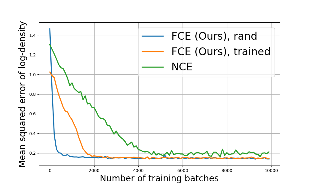
For the distribution depicted in the first row of Figure 1, which is a mixture of eight Gaussian distributions, we can compare the estimated densities by the learned models with the ground truth densities. Figure 2 shows the mean squared error of the estimated log-density over numbers of training iterations of EBMs. We show the results of FCE either starting from a randomly initialized Glow (’rand’) or a Glow model pre-trained by MLE (’trained’), and compare with NCE with a Gaussian noise distribution. FCE starting from a randomly initialized Glow converges in fewer iterations. Both settings of FCE achieve a lower error rate than NCE.
4.2 Learning on real image datasets
 |
 |
 |
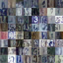
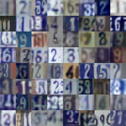
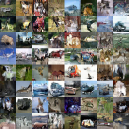
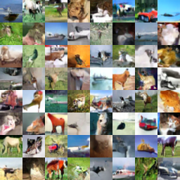
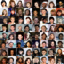
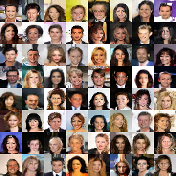
We conduct experiments on the Street View House Numbers (SVHN) [54], CIFAR-10 [35] and CelebA [45] datasets. We resized the CelebA images to pixels, and used images as a test set. We initialize FCE with a pre-trained Glow model, trained by MLE, for the sake of efficiency. We again emphasize the simplicity of the EBM model structure compared to Glow. See Appendix for detailed model architectures. For Glow, depth per level [32] is set as , , for SVHN, CelebA and CIFAR-10 respectively. Figure 3 depicts synthesized examples from learned Glow models. To evaluate the fidelity of synthesized examples, Table 1 summarizes the Fréchet Inception Distance (FID) [24] of the synthesized examples computed with the Inception V3 [67] classifier. The fidelity is significantly improved compared to Glow trained by MLE (see Appendix for qualitative comparisons), and is competitive to the other generative models. In Table 2, we report the average negative log-likelihood (bits per dimension) on the testing sets. The log-likelihood of the learned EBM is based on the estimated normalizing constant (i.e., a parameter of the model) and should be taken with a grain of salt. For the learned Glow model, the log-likelihood of the Glow model estimated with FCE is slightly lower than the log-likelihood of the Glow model trained with MLE.
| Method | SVHN | CIFAR-10 | CelebA |
|---|---|---|---|
| VAE [34] | 57.25 | 78.41 | 38.76 |
| DCGAN [59] | 21.40 | 37.70 | 12.50 |
| Glow [32] | 41.70 | 45.99 | 23.32 |
| FCE (Ours) | 20.19 | 37.30 | 12.21 |
| Model | SVHN | CIFAR-10 | CelebA |
|---|---|---|---|
| Glow-MLE | 2.17 | 3.35 | 3.49 |
| Glow-FCE (Ours) | 2.25 | 3.45 | 3.54 |
| EBM-FCE (Ours) | †2.15 | †3.27 | †3.40 |
4.3 Unsupervised feature learning
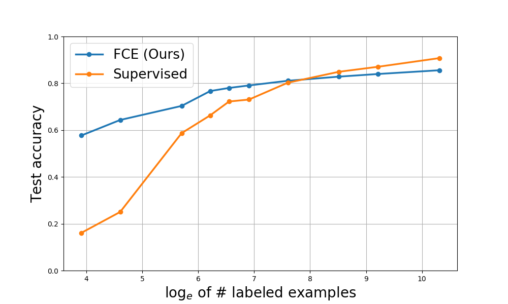
To further explore the EBM learned with FCE, we perform unsupervised feature learning with features from a learned EBM. Specifically, we first conduct FCE on the entire training set of SVHN in an unsupervised way. Then, we extract the top layer feature maps from the learned EBM, and train a linear classifier on top of the extracted features using only a subset of the training images and their corresponding labels. Figure 4 shows the classification accuracy as a function of the number of labeled examples. Meanwhile, we compare our method with a supervised model with the same model structure as the EBM, and is trained only on the same subset of labeled examples each time. We observe that FCE outperforms the supervised model when the number of labeled examples is small (less than ).
Next we try to combine features from multiple layers together. Specifically, following the same procedure outlined in [59], the features from the top three convolutional layers are max pooled and concatenated to form a -dimensional vector of feature. A regularized L2-SVM is then trained on these features with a subset of training examples and the corresponding labels. Table 3 summarizes the results of using , and labeled examples from the training set. At the top part of the table, we compare with methods that estimate an EBM or a discriminative model coupled with a generator network. At the middle part of the table, we compare with methods that learn an EBM with contrastive divergence (CD) and modified versions of CD. For fair comparison, we use the same model structure for the EBMs or discriminative models used in all the methods. The results indicate that FCE outperforms these methods in terms of the effectiveness of learned features.
| Method | # of labeled data | ||
|---|---|---|---|
| WGAN [1] | 43.15 | 38.00 | 32.56 |
| WGAN-GP [20] | 40.12 | 32.24 | 30.63 |
| DDGM [29] | 44.99 | 34.26 | 27.44 |
| DCGAN [59] | 38.59 | 32.51 | 29.37 |
| SN-GAN [49] | 40.82 | 31.24 | 28.69 |
| MMD-GAN-rep [74] | 36.74 | 29.12 | 25.23 |
| Persistent CD [69] | 45.74 | 39.47 | 34.18 |
| One-step CD [25] | 44.38 | 35.87 | 30.45 |
| Multigrid sampling [13] | 30.23 | 26.54 | 22.83 |
| FCE (Ours) | 27.07 | 24.12 | 22.05 |
4.4 Semi-supervised learning

In section 3.4 we show that FCE can be generalized to perform semi-supervised learning. We emphasize that for semi-supervised learning, FCE not only learns a classification boundary or a posterior label distribution . Instead, the algorithm ends up with estimated probabilistic distributions for observed examples belonging to categories. Figure 5 illustrates this point by showing the learning process on a 2D example, where the data distribution consists of two twisted spirals belonging to two categories. Seven labeled points are provided for each category. As the training goes, the unconditional EBM learns to capture all the modes of the data distribution, which is in the form of a mixture of class-conditional EBMs and . Meanwhile, by maximizing the objective function (eqn. 17), is forced to project the learned modes into different spaces, resulting in two well-separated class-conditional EBMs. As shown in Figure 5, within a single mode of one category, the EBM tends to learn a smoothly connected cluster, which is often what we desire in semi-supervised learning.
Then we test the proposed method on a dataset of real images. Following the setting in [50], we use two types of CNN structures (‘Conv-small’and ‘Conv-large’) for EBMs, which are commonly used in state-of-the-art semi-supervised learning methods. See Appendix for detailed model structures. We start FCE from a pre-trained Glow model. Before the joint training starts, EBMs are firstly trained for iterations with the Glow model fixed. In practice, this helps EBMs keep pace with the pre-trained Glow model, and equips EBMs with reasonable classification ability. We report the performance at this stage as ‘FCE-init’. Also, since virtual adversarial training (VAT) [50] has been demonstrated as an effective regularization method for semi-supervised learning, we consider adopting it as an additional loss for learning the EBMs. More specifically, the loss is defined as the robustness of the conditional label distribution around each input data point against local purturbation. ‘FCE + VAT’ indicates the training with VAT.
Table 4 summarizes the results of semi-supervised learning on SVHN dataset. We report the mean error rates and standard deviations over three runs. All the methods listed in the table belong to the family of semi-supervised learning methods. Our method achieve competitive performance to these state-of-the-art methods. ‘FCE + VAT’ results show that the effectiveness of FCE does not overlap much with existing semi-supervised method, and thus they can be combined to further boost the performance.
| Method | # of labeled data | |
|---|---|---|
| SWWAE [78] | 23.56 | |
| Skip DGM [46] | 16.61 | |
| Auxiliary DGM [46] | 22.86 | |
| GAN with FM [62] | 18.44 | 8.11 |
| VAT-Conv-small [50] | 6.83 | |
| on Conv-small used in [62, 50] | ||
| FCE-init | 9.42 | 8.50 |
| FCE | 7.05 | 6.35 |
| model [39] | 7.05 | 5.43 |
| VAT-Conv-large [50] | †8.98 | 5.77 |
| Mean Teacher [68] | 5.45 | 5.21 |
| model∗ [39] | 6.83 | 4.95 |
| Temporal ensembling∗ [39] | 5.12 | 4.42 |
| on Conv-large used in [39, 50] | ||
| FCE-init | 8.86 | 7.60 |
| FCE | 6.86 | 5.54 |
| FCE + VAT | 4.47 | 3.87 |
5 Conclusion
This paper explores joint training of an energy-based model with a flow-based model, by combining the representational flexibility of the energy-based model and the computational tractability of the flow-based model. We may consider the learned energy-based model as the learned representation, while the learned flow-based model as the learned computation. This method can be considered as an adaptive version of noise contrastive estimation where the noise is transformed by a flow model to make its distribution closer to the data distribution and to make it a stronger contrast to the energy-based model. Meanwhile, the flow-based model is updated adaptively through the learning process, under the same adversarial value function.
In future work, we intend to generalize the joint training method by combining the energy-based model with other normalized probabilistic models, such as auto-regressive models. We also intend to explore other joint training methods such as those based on adversarial contrastive divergence [29, 5, 22] or divergence triangle [22].
Acknowledgments
The work is partially supported by DARPA XAI project N66001-17-2-4029 and ARO project W911NF1810296. We thank Pavel Sountsov, Alex Alemi, Matthew D. Hoffman and Srinivas Vasudevan for their helpful discussions.
References
- [1] Martin Arjovsky, Soumith Chintala, and Bottou. Wasserstein gan. arXiv preprint arXiv:1701.07875, 2017.
- [2] Paul Baltescu and Phil Blunsom. Pragmatic neural language modelling in machine translation. arXiv preprint arXiv:1412.7119, 2014.
- [3] Jens Behrmann, David Duvenaud, and Jörn-Henrik Jacobsen. Invertible residual networks. arXiv preprint arXiv:1811.00995, 2018.
- [4] Avishek Joey Bose, Huan Ling, and Yanshuai Cao. Adversarial contrastive estimation. arXiv preprint arXiv:1805.03642, 2018.
- [5] Zihang Dai, Amjad Almahairi, Philip Bachman, Eduard Hovy, and Aaron Courville. Calibrating energy-based generative adversarial networks. arXiv preprint arXiv:1702.01691, 2017.
- [6] Guillaume Desjardins, Yoshua Bengio, and Aaron C Courville. On tracking the partition function. In Advances in neural information processing systems, pages 2501–2509, 2011.
- [7] Laurent Dinh, David Krueger, and Yoshua Bengio. Nice: Non-linear independent components estimation. arXiv preprint arXiv:1410.8516, 2014.
- [8] Laurent Dinh, Jascha Sohl-Dickstein, and Samy Bengio. Density estimation using real nvp. arXiv preprint arXiv:1605.08803, 2016.
- [9] Yilun Du and Igor Mordatch. Implicit generation and generalization in energy-based models. arXiv preprint arXiv:1903.08689, 2019.
- [10] Conor Durkan, Artur Bekasov, Iain Murray, and George Papamakarios. Neural spline flows. In Advances in Neural Information Processing Systems, pages 7509–7520, 2019.
- [11] Chelsea Finn, Paul Christiano, Pieter Abbeel, and Sergey Levine. A connection between generative adversarial networks, inverse reinforcement learning, and energy-based models. arXiv preprint arXiv:1611.03852, 2016.
- [12] Charles W Fox and Stephen J Roberts. A tutorial on variational bayesian inference. Artificial intelligence review, 38(2):85–95, 2012.
- [13] Ruiqi Gao, Yang Lu, Junpei Zhou, Song-Chun Zhu, and Ying Nian Wu. Learning generative convnets via multi-grid modeling and sampling. In Proceedings of the IEEE Conference on Computer Vision and Pattern Recognition, pages 9155–9164, 2018.
- [14] Mark Girolami and Ben Calderhead. Riemann manifold langevin and hamiltonian monte carlo methods. Journal of the Royal Statistical Society: Series B (Statistical Methodology), 73(2):123–214, 2011.
- [15] Ian Goodfellow, Jean Pouget-Abadie, Mehdi Mirza, Bing Xu, David Warde-Farley, Sherjil Ozair, Aaron Courville, and Yoshua Bengio. Generative adversarial nets. In Advances in neural information processing systems, pages 2672–2680, 2014.
- [16] Anirudh Goyal Alias Parth Goyal, Nan Rosemary Ke, Surya Ganguli, and Yoshua Bengio. Variational walkback: Learning a transition operator as a stochastic recurrent net. In Advances in Neural Information Processing Systems, pages 4392–4402, 2017.
- [17] Will Grathwohl, Ricky TQ Chen, Jesse Betterncourt, Ilya Sutskever, and David Duvenaud. Ffjord: Free-form continuous dynamics for scalable reversible generative models. arXiv preprint arXiv:1810.01367, 2018.
- [18] Will Grathwohl, Kuan-Chieh Wang, Jörn-Henrik Jacobsen, David Duvenaud, Mohammad Norouzi, and Kevin Swersky. Your classifier is secretly an energy based model and you should treat it like one. arXiv preprint arXiv:1912.03263, 2019.
- [19] Alex Graves. Generating sequences with recurrent neural networks. arXiv preprint arXiv:1308.0850, 2013.
- [20] Ishaan Gulrajani, Faruk Ahmed, Martin Arjovsky, Vincent Dumoulin, and Aaron C Courville. Improved training of wasserstein gans. In Advances in neural information processing systems, pages 5767–5777, 2017.
- [21] Michael Gutmann and Aapo Hyvärinen. Noise-contrastive estimation: A new estimation principle for unnormalized statistical models. In Proceedings of the Thirteenth International Conference on Artificial Intelligence and Statistics, pages 297–304, 2010.
- [22] Tian Han, Erik Nijkamp, Xiaolin Fang, Mitch Hill, Song-Chun Zhu, and Ying Nian Wu. Divergence triangle for joint training of generator model, energy-based model, and inference model. arXiv preprint arXiv:1812.10907, 2018.
- [23] Tianxing He, Yu Zhang, Jasha Droppo, and Kai Yu. On training bi-directional neural network language model with noise contrastive estimation. In 2016 10th International Symposium on Chinese Spoken Language Processing (ISCSLP), pages 1–5. IEEE, 2016.
- [24] Martin Heusel, Hubert Ramsauer, Thomas Unterthiner, Bernhard Nessler, and Sepp Hochreiter. Gans trained by a two time-scale update rule converge to a local nash equilibrium. In Advances in Neural Information Processing Systems, pages 6626–6637, 2017.
- [25] Geoffrey E Hinton. Training products of experts by minimizing contrastive divergence. Neural computation, 14(8):1771–1800, 2002.
- [26] Aapo Hyvärinen. Estimation of non-normalized statistical models by score matching. Journal of Machine Learning Research, 6(Apr):695–709, 2005.
- [27] Long Jin, Justin Lazarow, and Zhuowen Tu. Introspective classification with convolutional nets. In Advances in Neural Information Processing Systems, pages 823–833, 2017.
- [28] Ilyes Khemakhem, Diederik P Kingma, and Aapo Hyvärinen. Variational autoencoders and nonlinear ica: A unifying framework. arXiv preprint arXiv:1907.04809, 2019.
- [29] Taesup Kim and Yoshua Bengio. Deep directed generative models with energy-based probability estimation. arXiv preprint arXiv:1606.03439, 2016.
- [30] Diederik Kingma and Max Welling. In International Conference on Machine Learning, pages 1782–1790, 2014.
- [31] Diederik P Kingma and Jimmy Ba. Adam: A method for stochastic optimization. arXiv preprint arXiv:1412.6980, 2014.
- [32] Diederik P Kingma and Prafulla Dhariwal. Glow: Generative flow with invertible 1x1 convolutions. In Advances in Neural Information Processing Systems, pages 10215–10224, 2018.
- [33] Diederik P Kingma, Tim Salimans, Rafal Jozefowicz, Xi Chen, Ilya Sutskever, and Max Welling. Improved variational inference with inverse autoregressive flow. In Advances in neural information processing systems, pages 4743–4751, 2016.
- [34] Diederik P Kingma and Max Welling. Auto-encoding variational bayes. arXiv preprint arXiv:1312.6114, 2013.
- [35] Alex Krizhevsky, Geoffrey Hinton, et al. Learning multiple layers of features from tiny images. Technical report, Citeseer, 2009.
- [36] Alex Krizhevsky, Ilya Sutskever, and Geoffrey E Hinton. Imagenet classification with deep convolutional neural networks. In Advances in neural information processing systems, pages 1097–1105, 2012.
- [37] Manoj Kumar, Mohammad Babaeizadeh, Dumitru Erhan, Chelsea Finn, Sergey Levine, Laurent Dinh, and Durk Kingma. Videoflow: A flow-based generative model for video. arXiv preprint arXiv:1903.01434, 2019.
- [38] Rithesh Kumar, Anirudh Goyal, Aaron Courville, and Yoshua Bengio. Maximum entropy generators for energy-based models. arXiv preprint arXiv:1901.08508, 2019.
- [39] Samuli Laine and Timo Aila. Temporal ensembling for semi-supervised learning. arXiv preprint arXiv:1610.02242, 2016.
- [40] Justin Lazarow, Long Jin, and Zhuowen Tu. Introspective neural networks for generative modeling. In Proceedings of the IEEE International Conference on Computer Vision, pages 2774–2783, 2017.
- [41] Yann LeCun, Léon Bottou, Yoshua Bengio, Patrick Haffner, et al. Gradient-based learning applied to document recognition. Proceedings of the IEEE, 86(11):2278–2324, 1998.
- [42] Yann LeCun, Sumit Chopra, Raia Hadsell, M Ranzato, and F Huang. A tutorial on energy-based learning. Predicting structured data, 1(0), 2006.
- [43] Kwonjoon Lee, Weijian Xu, Fan Fan, and Zhuowen Tu. Wasserstein introspective neural networks. In Proceedings of the IEEE Conference on Computer Vision and Pattern Recognition, pages 3702–3711, 2018.
- [44] Sergey Levine and Vladlen Koltun. Guided policy search. In International Conference on Machine Learning, pages 1–9, 2013.
- [45] Ziwei Liu, Ping Luo, Xiaogang Wang, and Xiaoou Tang. Large-scale celebfaces attributes (celeba) dataset. Retrieved August, 15:2018, 2018.
- [46] Lars Maaløe, Casper Kaae Sønderby, Søren Kaae Sønderby, and Ole Winther. Auxiliary deep generative models. arXiv preprint arXiv:1602.05473, 2016.
- [47] Andrew L Maas, Awni Y Hannun, and Andrew Y Ng. Rectifier nonlinearities improve neural network acoustic models. In Proc. icml, volume 30, page 3, 2013.
- [48] Tomas Mikolov, Ilya Sutskever, Kai Chen, Greg S Corrado, and Jeff Dean. Distributed representations of words and phrases and their compositionality. In Advances in neural information processing systems, pages 3111–3119, 2013.
- [49] Takeru Miyato, Toshiki Kataoka, Masanori Koyama, and Yuichi Yoshida. Spectral normalization for generative adversarial networks. arXiv preprint arXiv:1802.05957, 2018.
- [50] Takeru Miyato, Shin-ichi Maeda, Masanori Koyama, and Shin Ishii. Virtual adversarial training: a regularization method for supervised and semi-supervised learning. IEEE transactions on pattern analysis and machine intelligence, 41(8):1979–1993, 2018.
- [51] Andriy Mnih and Koray Kavukcuoglu. Learning word embeddings efficiently with noise-contrastive estimation. In Advances in neural information processing systems, pages 2265–2273, 2013.
- [52] Andriy Mnih and Yee Whye Teh. A fast and simple algorithm for training neural probabilistic language models. arXiv preprint arXiv:1206.6426, 2012.
- [53] Kevin P Murphy. Machine learning: a probabilistic perspective. MIT press, 2012.
- [54] Yuval Netzer, Tao Wang, Adam Coates, Alessandro Bissacco, Bo Wu, and Andrew Y Ng. Reading digits in natural images with unsupervised feature learning. 2011.
- [55] Jiquan Ngiam, Zhenghao Chen, Pang W Koh, and Andrew Y Ng. Learning deep energy models. In Proceedings of the 28th international conference on machine learning (ICML-11), pages 1105–1112, 2011.
- [56] Erik Nijkamp, Mitch Hill, Song-Chun Zhu, and Ying Nian Wu. On learning non-convergent short-run mcmc toward energy-based model. arXiv preprint arXiv:1904.09770, 2019.
- [57] Aaron van den Oord, Sander Dieleman, Heiga Zen, Karen Simonyan, Oriol Vinyals, Alex Graves, Nal Kalchbrenner, Andrew Senior, and Koray Kavukcuoglu. Wavenet: A generative model for raw audio. arXiv preprint arXiv:1609.03499, 2016.
- [58] Youssef Oualil and Dietrich Klakow. A batch noise contrastive estimation approach for training large vocabulary language models. arXiv preprint arXiv:1708.05997, 2017.
- [59] Alec Radford, Luke Metz, and Soumith Chintala. Unsupervised representation learning with deep convolutional generative adversarial networks. arXiv preprint arXiv:1511.06434, 2015.
- [60] Danilo Jimenez Rezende and Shakir Mohamed. Variational inference with normalizing flows. arXiv preprint arXiv:1505.05770, 2015.
- [61] Danilo Jimenez Rezende, Shakir Mohamed, and Daan Wierstra. Stochastic backpropagation and approximate inference in deep generative models. arXiv preprint arXiv:1401.4082, 2014.
- [62] Tim Salimans, Ian Goodfellow, Wojciech Zaremba, Vicki Cheung, Alec Radford, and Xi Chen. Improved techniques for training gans. In Advances in neural information processing systems, pages 2234–2242, 2016.
- [63] Tim Salimans, Andrej Karpathy, Xi Chen, and Diederik P Kingma. Pixelcnn++: Improving the pixelcnn with discretized logistic mixture likelihood and other modifications. arXiv preprint arXiv:1701.05517, 2017.
- [64] Tim Salimans and Durk P Kingma. Weight normalization: A simple reparameterization to accelerate training of deep neural networks. In Advances in Neural Information Processing Systems, pages 901–909, 2016.
- [65] Saeed Saremi, Arash Mehrjou, Bernhard Schölkopf, and Aapo Hyvärinen. Deep energy estimator networks. arXiv preprint arXiv:1805.08306, 2018.
- [66] Yang Song and Stefano Ermon. Generative modeling by estimating gradients of the data distribution. In Advances in Neural Information Processing Systems, pages 11895–11907, 2019.
- [67] Christian Szegedy, Vincent Vanhoucke, Sergey Ioffe, Jon Shlens, and Zbigniew Wojna. Rethinking the inception architecture for computer vision. In Proceedings of the IEEE conference on computer vision and pattern recognition, pages 2818–2826, 2016.
- [68] Antti Tarvainen and Harri Valpola. Mean teachers are better role models: Weight-averaged consistency targets improve semi-supervised deep learning results. In Advances in neural information processing systems, pages 1195–1204, 2017.
- [69] Tijmen Tieleman. Training restricted boltzmann machines using approximations to the likelihood gradient. In Proceedings of the 25th international conference on Machine learning, pages 1064–1071. ACM, 2008.
- [70] Dustin Tran, Keyon Vafa, Kumar Krishna Agrawal, Laurent Dinh, and Ben Poole. Discrete flows: Invertible generative models of discrete data. arXiv preprint arXiv:1905.10347, 2019.
- [71] Zhuowen Tu. Learning generative models via discriminative approaches. In 2007 IEEE Conference on Computer Vision and Pattern Recognition, pages 1–8. IEEE, 2007.
- [72] Ashish Vaswani, Yinggong Zhao, Victoria Fossum, and David Chiang. Decoding with large-scale neural language models improves translation. In Proceedings of the 2013 Conference on Empirical Methods in Natural Language Processing, pages 1387–1392, 2013.
- [73] Ivan Vendrov, Ryan Kiros, Sanja Fidler, and Raquel Urtasun. Order-embeddings of images and language. arXiv preprint arXiv:1511.06361, 2015.
- [74] Wei Wang, Yuan Sun, and Saman Halgamuge. Improving mmd-gan training with repulsive loss function. arXiv preprint arXiv:1812.09916, 2018.
- [75] Jianwen Xie, Yang Lu, Song-Chun Zhu, and Yingnian Wu. A theory of generative convnet. In International Conference on Machine Learning, pages 2635–2644, 2016.
- [76] Shuangfei Zhai, Yu Cheng, Weining Lu, and Zhongfei Zhang. Deep structured energy based models for anomaly detection. arXiv preprint arXiv:1605.07717, 2016.
- [77] Shuangfei Zhai, Walter Talbott, Carlos Guestrin, and Joshua Susskind. Adversarial fisher vectors for unsupervised representation learning. In Advances in Neural Information Processing Systems, pages 11156–11166, 2019.
- [78] Junbo Zhao, Michael Mathieu, Ross Goroshin, and Yann Lecun. Stacked what-where auto-encoders. arXiv preprint arXiv:1506.02351, 2015.
- [79] Junbo Zhao, Michael Mathieu, and Yann LeCun. Energy-based generative adversarial network. arXiv preprint arXiv:1609.03126, 2016.
- [80] Song Chun Zhu and David Mumford. Grade: Gibbs reaction and diffusion equations. In Sixth International Conference on Computer Vision (IEEE Cat. No. 98CH36271), pages 847–854. IEEE, 1998.
Appendix A Model architectures
Table 5 summarizes the EBM architectures used in unsupervised learning (subsections 4.1-4.3). The slope of all leaky ReLU (lReLU) [47] functions are set to . For semi-supervised learning from a 2D example (subsection 4.4), we use the same EBM structure as the one used in unsupervised learning from 2D examples, except that for the top fully connect layer, we change the number of output channels to , to model EBMs of two categories respectively. Table 6 summarizes the EBM architectures used in semi-supervised learning from SVHN (subsection 4.4). After each convolutional layer, a weight normalization [64] layer and a leaky ReLU layer is added. The slope of leaky ReLU functions is set to . A weight normalization layer is added after the top fully connected layer.
| 2D data | SVHN / CIFAR-10 |
|---|---|
| fc. lReLU | conv. lReLU, stride |
| fc. lReLU | conv. lReLU, stride |
| fc. lReLU | conv. lReLU, stride |
| fc. | conv. , stride |
| Conv-small | Conv-large |
|---|---|
| dropout, | |
| conv. , stride | conv. , stride |
| conv. , stride | conv. , stride |
| conv. , stride | conv. , stride |
| dropout, | |
| conv. , stride | conv. , stride |
| conv. , stride | conv. , stride |
| conv. , stride | conv. , stride |
| dropout, | |
| conv. , stride | conv. , stride |
| conv. , stride | conv. , stride |
| conv. , stride | conv. , stride |
| global max pool, | |
| fc. | |
For Glow model, we follow the setting of [32]. The architecture has multi-scales with levels . Within each level, there are flow blocks. Each block has three convolutional layers (or fully-connected layers) with a width of channels. After the first two layers, a ReLU activation is added. Table 7 summarizes the hyperparameters for different datasets.
| Dataset | Levels | Blocks per level | Width | Layer type | Coupling |
|---|---|---|---|---|---|
| 2D data | 1 | 10 | 128 | fc | affine |
| SVHN | 3 | 8 | 512 | conv | additive |
| CelebA | 3 | 16 | 512 | conv | additive |
| CIFAR-10 | 3 | 32 | 512 | conv | additive |
Appendix B Synthesis comparison
