Energy dissipation for hereditary and
energy conservation for non-local fractional wave equations

Abstract

Using the method of a priori energy estimates, energy dissipation is proved for the class of hereditary fractional wave equations, obtained through the system of equations consisting of equation of motion, strain, and fractional order constitutive models, that include the distributed-order constitutive law in which the integration is performed from zero to one generalizing all linear constitutive models of fractional and integer orders, as well as for the thermodynamically consistent fractional Burgers models, where the orders of fractional differentiation are up to the second order. In the case of non-local fractional wave equations, obtained using non-local constitutive models of Hooke- and Eringen-type in addition to the equation of motion and strain, a priori energy estimates yield the energy conservation, with the reinterpreted notion of the potential energy.

Key words: fractional wave equation, hereditary and non-local fractional constitutive equations, energy dissipation and conservation

1 Introduction

Fractional wave equations, describing the disturbance propagation in a viscoelastic or non-local material, are obtained through the system of equations consisting of: equation of motion corresponding to one-dimensional deformable body

$$\partial_{x}\sigma(x,t)=\rho\,\partial_{tt}u(x,t),$$ (1)

where $u$ and $\sigma$ are displacement and stress, assumed as functions of space $x\in\mathbb{R}$ and time $t>0,$ with $\rho$ being constant material density, strain for small local deformations

$$\varepsilon(x,t)=\partial_{x}u(x,t),$$ (2)

and constitutive equation connecting stress and strain, which can model either hereditary or non-local material properties.

The aim is to investigate the energy conserving properties of such obtained wave equations, namely hereditary and non-local wave equations. Hereditary materials are modelled by the fractional-order constitutive equations of viscoelastic body including distributed-order model containing fractional differentiation orders up to the first order, as well as fractional Burgers models containing also the differentiation orders up to the second order. Energy dissipation is expected for hereditary wave equations, since the thermodynamical requirements on the model parameters impose dissipativity of such constitutive models. On the other hand, non-local materials, modelled by the non-local Hooke law and fractional Eringen stress gradient model, are not expected to dissipate energy.

Hereditary effects in a viscoelastic body are modelled either by the distributed-order constitutive equation

$$\int_{0}^{1}\phi_{\sigma}(\alpha)\,{}_{0}\mathrm{D}_{t}^{\alpha}\sigma(x,t)\,\mathrm{d}\alpha=\int_{0}^{1}\phi_{\varepsilon}(\alpha)\,{}_{0}\mathrm{D}_{t}^{\alpha}\varepsilon(x,t)\,\mathrm{d}\alpha,$$ (3)

where $\phi_{\sigma}$ and $\phi_{\varepsilon}$ are constitutive functions or distributions and where fractional differentiation orders do not exceed the first order, or by the thermodynamically consistent fractional Burgers models where fractional differentiation orders are up to the second order. The fractional Burgers models are represented by unified models belonging to two classes: the first class is represented by the unified constitutive equation

$$\left(1+a_{1}\,{}_{0}\mathrm{D}_{t}^{\alpha}+a_{2}\,{}_{0}\mathrm{D}_{t}^{\beta}+a_{3}\,{}_{0}\mathrm{D}_{t}^{\gamma}\right)\sigma\left(x,t\right)=\left(b_{1}\,{}_{0}\mathrm{D}_{t}^{\mu}+b_{2}\,{}_{0}\mathrm{D}_{t}^{\mu+\eta}\right)\varepsilon\left(x,t\right),$$ (4)

while the second one is represented by

$$\left(1+a_{1}\,{}_{0}\mathrm{D}_{t}^{\alpha}+a_{2}\,{}_{0}\mathrm{D}_{t}^{\beta}+a_{3}\,{}_{0}\mathrm{D}_{t}^{\beta+\eta}\right)\sigma\left(x,t\right)=\left(b_{1}\,{}_{0}\mathrm{D}_{t}^{\beta}+b_{2}\,{}_{0}\mathrm{D}_{t}^{\beta+\eta}\right)\varepsilon\left(x,t\right),$$ (5)

where $a_{1},a_{2},a_{3},b_{1},b_{2}>0,$ $\alpha,\beta,\mu\in\left[0,1\right],$ with $\alpha\leq\beta,$ $\gamma\in\left[0,2\right],$ and $\eta\in\left\{\alpha,\beta\right\}.$ The operator of Riemann-Liouville fractional derivative ${}_{0}\mathrm{D}_{t}^{\xi}$ of order $\xi\in\left[n,n+1\right],$ $n\in\mathbb{N}_{0},$ used in constitutive models (3), (4), and (5), is defined by

$${}_{0}\mathrm{D}_{t}^{\xi}y\left(t\right)=\frac{\mathrm{d}^{n+1}}{\mathrm{d}t^{n+1}}\left(\frac{t^{-\left(\xi-n\right)}}{\Gamma\left(1-\left(\xi-n\right)\right)}\ast_{t}y\left(t\right)\right),\;\;t>0,$$

see [23], where $\ast_{t}$ denotes the convolution in time: $f\left(t\right)\ast_{t}g\left(t\right)=\int_{0}^{t}f\left(t^{\prime}\right)g\left(t-t^{\prime}\right)\mathrm{d}t^{\prime},$ $t>0.$

Non-locality effects in a material are described either by the non-local Hooke law

$$\sigma(x,t)=\frac{E}{\ell^{1-\alpha}}\frac{|x|^{-\alpha}}{2\Gamma(1-\alpha)}\ast_{x}\varepsilon(x,t),\;\;\alpha\in\left(0,1\right),$$ (6)

or by the fractional Eringen constitutive equation

$$\sigma\left(x,t\right)-\ell^{\alpha}\,\mathrm{D}_{x}^{\alpha}\sigma\left(x,t\right)=E\,\varepsilon\left(x,t\right),\;\;\alpha\in\left(1,3\right),$$ (7)

where $E$ is Young modulus, $\ell$ is non-locality parameter, and $\mathrm{D}_{x}^{\alpha}$ is defined as

$$\mathrm{D}_{x}^{\alpha}y\left(x\right) = \frac{\left|x\right|^{1-\alpha}}{2\Gamma\left(2-\alpha\right)}\ast_{x}\frac{\mathrm{d}^{2}}{\mathrm{d}x^{2}}y\left(x\right),\;\;\text{for}\;\;\alpha\in\left(1,2\right),$$ (8)

$$\mathrm{D}_{x}^{\alpha}y\left(x\right) = \frac{\left|x\right|^{2-\alpha}\mathop{\mathrm{s}gn}x}{2\Gamma\left(3-\alpha\right)}\ast_{x}\frac{\mathrm{d}^{3}}{\mathrm{d}x^{3}}y\left(x\right),\;\;\text{for}\;\;\alpha\in\left(2,3\right),$$ (9)

with $\ast_{x}$ denoting the convolution in space: $f\left(x\right)\ast_{x}g\left(x\right)=\int_{\mathbb{R}}f\left(x^{\prime}\right)g\left(x-x^{\prime}\right)\mathrm{d}x^{\prime},$ $x\in\mathbb{R}.$

The Cauchy problem on the real line $x\in\mathbb{R}$ and $t>0$ is considered, so the system of governing equations (1), (2), and one of the constitutive equations (3), or (4), or (5), or (6), or (7) is subject to initial and boundary conditions:

$$u(x,0)=u_{0}(x),\;\;\frac{\partial}{\partial t}u(x,0)=v_{0}(x),$$ (10)

$$\sigma(x,0)=0,\;\;\varepsilon(x,0)=0,\;\;\partial_{t}\sigma(x,0)=0,\;\;\partial_{t}\varepsilon(x,0)=0,$$ (11)

$$\lim_{x\rightarrow\pm\infty}u(x,t)=0,\;\;\lim_{x\rightarrow\pm\infty}\sigma(x,t)=0,$$ (12)

where $u_{0}$ is the initial displacement and $v_{0}$ is the initial velocity. The initial conditions (11) are needed for the hereditary constitutive equations: distributed-order constitutive equation (3) needs (11)_1,2 and fractional Burgers models (4), (5) require all initial conditions (11), while non-local constitutive models (6) and (7) do not need any of the initial conditions (11).

The distributed-order constitutive model (3) generalizes integer and fractional order constitutive models of linear viscoelasticity having differentiation orders up to the first order, since it reduces to the linear fractional model

$$\sum_{i=1}^{n}a_{i}\,{}_{0}\mathrm{D}_{t}^{\alpha_{i}}\sigma(x,t)=\sum_{j=1}^{m}b_{j}\,{}_{0}\mathrm{D}_{t}^{\beta_{j}}\varepsilon(x,t),$$ (13)

with model parameters $a_{i},b_{j}>0$ and $\alpha_{i},\beta_{j}\in\left[0,1\right],$ $i=1,\ldots,n$, $j=1,\ldots,m,$ if the constitutive distributions $\phi_{\sigma}$ and $\phi_{\varepsilon}$ in (3) are chosen as

$$\phi_{\sigma}(\alpha)=\sum_{i=1}^{n}a_{i}\,\delta(\alpha-\alpha_{i}),\;\;\phi_{\varepsilon}(\alpha)=\sum_{j=1}^{m}b_{i}\,\delta(\alpha-\beta_{j}),$$

where $\delta$ denotes the Dirac delta distribution. Moreover, the power-type distributed-order model

$$\int_{0}^{1}a^{\alpha}\,{}_{0}\mathrm{D}_{t}^{\alpha}\sigma(x,t)\,\mathrm{d}\alpha=E\int_{0}^{1}b^{\alpha}\,{}_{0}\mathrm{D}_{t}^{\alpha}\varepsilon(x,t)\,\mathrm{d}\alpha,$$ (14)

is obtained from (3) as the genuine distributed-order model, if constitutive functions $\phi_{\sigma}$ and $\phi_{\varepsilon}$ in (3) are chosen as

$$\phi_{\sigma}(\alpha)=a^{\alpha},\;\;\phi_{\varepsilon}(\alpha)=E\,b^{\alpha},$$

with model parameters $E,a,b>0$ ensuring dimensional homogeneity.

Thermodynamical consistency of linear fractional constitutive equation (13) is examined in [3], where it is shown that there are four cases of (13) when the restrictions on model parameters guarantee its thermodynamical consistency, while power-type distributed-order model (14) is considered in [1] and revisited in [3], where the conditions $E>0$ and $0\leq a\leq b,$ guaranteeing model’s thermodynamical consistency, are obtained. Four cases of thermodynamically acceptable models corresponding to (13) are given in Appendix A.

Fractional wave equations, corresponding to the system of governing equations (1), (2), and distributed-order constitutive model (3), are considered for the Cauchy problem in [26], generalizing the results of [24, 25], where respectively fractional Zener model and its generalization

$$\left(1+a\,{}_{0}\mathrm{D}_{t}^{\alpha}\right)\sigma(x,t)=E\left(1+b\,{}_{0}\mathrm{D}_{t}^{\alpha}\right)\varepsilon(x,t),\;\;0\leq a\leq b,\;\alpha\in\left[0,1\right],$$ (15)

$$\sum_{i=1}^{n}a_{i}\,{}_{0}\mathrm{D}_{t}^{\alpha_{i}}\sigma(x,t)=\sum_{i=1}^{n}b_{i}\,{}_{0}\mathrm{D}_{t}^{\alpha_{i}}\varepsilon(x,t),\;\;0\leq\alpha_{1}\leq\ldots\leq\alpha_{n}<1,\;\frac{a_{1}}{b_{1}}\geq\ldots\geq\frac{a_{n}}{b_{n}}\geq 0,$$

are considered as special cases of (13). Considering the wave propagation speed, it is found in [26] that the finite wave speed, so as the infinite, is the property of both solid-like and fluid-like materials. Solid-like and fluid-like materials are differed in the creep test, representing the deformation response of a material to a sudden but later on constant stress, where the deformation for first type of materials is bounded for large time in contrary to the second type of materials that have unbounded deformation for large time.

Eight thermodynamically consistent fractional Burgers models, formulated in [30], all describing fluid-like material behavior are divided into two classes. The first class, represented by (4), contains five models, such that the highest fractional differentiation order of strain is $\mu+\eta\in\left[1,2\right],$ with $\eta\in\left\{\alpha,\beta\right\},$ while the highest fractional differentiation order of stress is either $\gamma\in\left[0,1\right]$ in the case of Model I, with $0\leq\alpha\leq\beta\leq\gamma\leq\mu\leq 1$ and $\eta\in\left\{\alpha,\beta,\gamma\right\},$ or $\gamma\in\left[1,2\right]$ in the case of Models II - V, with $0\leq\alpha\leq\beta\leq\mu\leq 1$ and $\left(\eta,\gamma\right)\in\left\{\left(\alpha,2\alpha\right),\left(\alpha,\alpha+\beta\right),\left(\beta,\alpha+\beta\right),\left(\beta,2\beta\right)\right\}$. Note that the fractional differentiation order of stress is less than the differentiation order of strain regardless on the interval $\left[0,1\right]$ or $\left[1,2\right].$ The second class, represented by (5), contains three models, such that $0\leq\alpha\leq\beta\leq 1$ and $\beta+\eta\in\left[1,2\right],$ with $\eta=\alpha,$ in the case of Model VI; $\eta=\beta$ in the case of Model VII; and $\alpha=\eta=\beta,$ $\bar{a}_{1}=a_{1}+a_{2},$ and $\bar{a}_{2}=a_{3}$ in the case of Model VIII. Note that considering the interval $\left[0,1\right],$ the highest fractional differentiation orders of stress and strain are equal, which also holds true for the orders from interval $\left[1,2\right].$ The explicit forms of Models I - VIII, along with corresponding thermodynamical restrictions, can be found in Appendix B.

Fractional Burgers wave equation, represented by the governing equations (1), (2), and either (4) or (5), is solved for the Cauchy problem in [33]. The wave propagation speed is found to be infinite for models belonging to the first class, given by (4), contrary to the case of models of the second class (5), that yield finite wave propagation speed. Moreover, numerical examples indicated that at the wave front there might exist a jump from finite to a zero value of displacement, obtained as the fundamental solution of the fractional Burgers equation.

The non-local Hooke law (6) is introduced in [5] through the non-local strain measure and used with the classical Hooke law as a constitutive equation for modeling wave propagation in non-local media, while in [2] the constitutive equation including both memory and non-local effects is constructed using fractional Zener model (15) and non-local Hooke law (6), further to be used in describing wave propagation in non-local viscoelastic material. The tools of microlocal analysis are employed in [21] to investigate properties of this memory and non-local type fractional wave equation.

Generalizing the integer-order Eringen stress gradient non-local constitutive law, the fractional Eringen model (7) is postulated in [11], where the optimal values of non-locality parameter and order of fractional differentiation are obtained with respect to the Born-Kármán model of lattice dynamics. Further, wave propagation, as well as propagation of singularities, in non-local material described by the fractional Eringen model (7) is analyzed in [22].

The energy estimates for proving existence and uniqueness of the solution to three-dimensional wave equation corresponding to material of fractional Zener type using the Galerkin method are considered in [32, 34], while three-dimensional wave equation as a singular kernel integrodifferential equation, with kernel being the relaxation modulus unbounded at the initial time, is analyzed in [9]. The positivity of Green’s functions corresponding to a three-dimensional integrodifferential wave equation, that has completely monotonic relaxation modulus as a kernel, is established in [19], while the exponential energy decay of non-linear viscoelastic wave equation under the potential well is analyzed in [37] assuming Dirichlet boundary conditions.

In the case of one-dimensional wave equation, written as the integrodifferential equation including the relaxation modulus assumed as a wedge continuous function, the solution existence and uniqueness analysis is performed in [10], while [8] aimed to underline the similarities between rigid heat conductor having heat flux relaxation function singular at the origin and viscoelastic material having relaxation modulus unbounded at the origin. In [14, 18] one-dimensional wave propagation characteristics, such as wave propagation speed and wave attenuation, are investigated without and with the Newtonian viscosity component present in the completely monotonic relaxation modulus. The extensive overview of wave propagation problems in viscoelastic materials can be found in [4, 20, 27].

In [38] the transient effects, i.e., short-lived seismic wave propagation through viscoelastic subsurface media, are considered and asymptotic expansions of the solutions via Buchen-Mainardi algorithm method introduced in [6] are obtained. The same method is used in [12] in the case of waves in fractional Maxwell and Kelvin-Voigt viscoelastic materials. Dispersion, attenuation, wave fronts, and asymptotic behavior of solution to viscoelastic wave equation near the wave front are studied in [15, 16, 17].

The survey of acoustic wave equations aiming to describe the frequency dependent attenuation and scattering of acoustic disturbance propagation through complex media displaying viscous dissipation is presented in [7], while the frequency responses of viscoelastic materials are reviewed in [28].

The existence and uniqueness of solutions to three-dimensional wave equation with the Eringen model as a constitutive equation is studied in [13] and it is found that the problem is in general ill-posed in the case of smooth kernels and well-posed in the case of singular, non-smooth kernels. Considering the longitudinal and shear waves propagation in non-local medium, the influence of geometric non-linearity is investigated in [29]. Combining viscoelastic and non-locality characteristics of the medium, the wave propagation and wave decay is studied in [35] under the source positioned at the end of a semi-infinite medium.

2 Hereditary fractional wave equations expressed through relaxation modulus and creep compliance

Relaxation modulus and creep compliance, representing material properties in stress relaxation and creep tests, are used in order to formulate fractional wave equation corresponding to the system of governing equations (1), (2), and (3), or (4), or (5).

Relaxation modulus $\sigma_{sr}$ (creep compliance $\varepsilon_{cr}$) is the stress (strain) history function obtained as a response to the strain (stress) assumed as the Heaviside step function $H.$ According to the material behavior in stress relaxation and creep tests at the initial time-instant, one differs the materials having either finite or infinite glass modulus $\sigma_{sr}^{\left(g\right)}=\sigma_{sr}\left(0\right),$ implying the finite or zero value of the glass compliance $\varepsilon_{cr}^{\left(g\right)}=\varepsilon_{cr}\left(0\right).$ The wave propagation speed, obtained as

$$c=\sqrt{\sigma_{sr}^{\left(g\right)}}=\frac{1}{\sqrt{\varepsilon_{cr}^{\left(g\right)}}}$$

in [26] for the distributed-order constitutive model (3) and in [33] for the fractional Burgers models (4) and (5), is the implication of these material properties. On the other hand, according to the material behavior in stress relaxation and creep tests for large time, one differs fluid-like materials, having the equilibrium compliance $\varepsilon_{cr}^{\left(e\right)}=\lim_{t\rightarrow\infty}\varepsilon_{cr}\left(t\right)$ infinite and therefore the equilibrium modulus $\sigma_{sr}^{\left(e\right)}=\lim_{t\rightarrow\infty}\sigma_{sr}\left(t\right)$ zero, from solid-like materials, having both equilibrium compliance and equilibrium modulus finite. The overview of asymptotic properties for viscoelastic materials described by constitutive models (3), (4), and (5) is presented in Table 1.

[.5]0 Model	Material type	Wave speed	$\sigma_{sr}^{\left(g\right)}$	$\varepsilon_{cr}^{\left(g\right)}$	$\sigma_{sr}^{\left(e\right)}$	$\varepsilon_{cr}^{\left(e\right)}$
[.5]0 Power-type	solid-like	finite	$\frac{Eb}{a}$	$\frac{a}{Eb}$	$E$	$\frac{1}{E}$
[.5]0 Case I			$\frac{b_{n}}{a_{n}}$	$\frac{a_{n}}{b_{n}}$	$\frac{b_{1}}{a_{1}}$	$\frac{a_{1}}{b_{1}}$
[.5]0 Case II		infinite	$\infty$	$0$	$\frac{b_{1}}{a_{1}}$	$\frac{a_{1}}{b_{1}}$
[.5]0 Case III	fluid-like	finite	$\frac{b_{n}}{a_{n}}$	$\frac{a_{n}}{b_{n}}$	$0$	$\infty$
[.5]0 Case IV		infinite	$\infty$	$0$	$0$	$\infty$
[.5]0 Models I - V			$\infty$	$0$	$0$	$\infty$
[.5]0 Models VI - VIII		finite	$\frac{b_{2}}{a_{3}}$	$\frac{a_{3}}{b_{2}}$	$0$	$\infty$

Table 1: Summary of models’ properties.

In order to express the constitutive equations (3), (4), and (5) either in terms of the relaxation modulus, or in terms of the creep compliance, the Laplace transform with respect to time

$$\tilde{f}\left(s\right)=\mathcal{L}\left[f\left(t\right)\right]\left(s\right)=\int_{0}^{\infty}f\left(t\right)\mathrm{e}^{-st}\,\mathrm{d}t,\;\;\mathop{\mathrm{R}e}s>0,$$

is applied to (3), (4), and (5), so that

$$\Phi_{\sigma}(s)\tilde{\sigma}\left(x,s\right)=\Phi_{\varepsilon}(s)\tilde{\varepsilon}\left(x,s\right),\;\;\mathop{\mathrm{R}e}s>0,$$ (16)

is obtained assuming zero initial conditions (11), with

$$\Phi_{\sigma}(s)=\int_{0}^{1}\phi_{\sigma}(\alpha)s^{\alpha}\,\mathrm{d}\alpha,\;\;\Phi_{\varepsilon}(s)=\int_{0}^{1}\phi_{\varepsilon}(\alpha)s^{\alpha}\,\mathrm{d}\alpha,$$ (17)

in the case distributed-order constitutive model (3), reducing to

$$\Phi_{\sigma}(s)=\sum_{i=1}^{n}a_{i}\,s^{\alpha_{i}},\;\;\Phi_{\varepsilon}(s)=\sum_{j=1}^{m}b_{j}\,s^{\beta_{j}},\;\;\text{and}\;\;\Phi_{\sigma}(s)=\frac{as-1}{\ln\left(as\right)},\;\;\Phi_{\varepsilon}(s)=E\frac{bs-1}{\ln\left(bs\right)},$$ (18)

for linear fractional constitutive equation (13) and power-type distributed-order model (14), respectively, as well as with

$$\Phi_{\sigma}(s)=1+a_{1}s^{\alpha}+a_{2}\,s^{\beta}+a_{3}\,s^{\gamma},\;\;\Phi_{\varepsilon}(s)=b_{1}\,s^{\mu}+b_{2}\,s^{\mu+\eta},$$ (19)

$$\Phi_{\sigma}(s)=1+a_{1}s^{\alpha}+a_{2}\,s^{\beta}+a_{3}\,s^{\beta+\eta},\;\;\Phi_{\varepsilon}(s)=b_{1}\,s^{\beta}+b_{2}\,s^{\beta+\eta},$$ (20)

in the case of fractional Burgers model of the first, respectively second class, given by (4) and (5).

The Laplace transform of relaxation modulus and creep compliance

$$\tilde{\sigma}_{sr}\left(s\right)=\frac{1}{s}\frac{\Phi_{\varepsilon}(s)}{\Phi_{\sigma}(s)}\;\;\text{and}\;\;\tilde{\varepsilon}_{cr}\left(s\right)=\frac{1}{s}\frac{\Phi_{\sigma}(s)}{\Phi_{\varepsilon}(s)}$$ (21)

are respectively obtained by using the Laplace transform of constitutive equation (16) for $\tilde{\varepsilon}\left(x,s\right)=\mathcal{L}\left[H\left(t\right)\right]\left(s\right)=\frac{1}{s}$ and $\tilde{\sigma}\left(x,s\right)=\mathcal{L}\left[H\left(t\right)\right]\left(s\right)=\frac{1}{s},$ so that (21) used in (16) yielded the Laplace transform of constitutive equation (16) expressed either in terms of relaxation modulus, or in terms of creep compliance as

$$\frac{1}{s}\tilde{\sigma}\left(x,s\right)=\tilde{\sigma}_{sr}\left(s\right)\tilde{\varepsilon}\left(x,s\right)\;\;\text{or}\;\;\frac{1}{s}\tilde{\varepsilon}\left(x,s\right)=\tilde{\varepsilon}_{cr}\left(s\right)\tilde{\sigma}\left(x,s\right),$$ (22)

providing six equivalent forms of the hereditary constitutive equation: three expressed in terms of relaxation modulus

$$\int_{0}^{t}\sigma\left(x,t^{\prime}\right)\mathrm{d}t^{\prime}=\sigma_{sr}\left(t\right)\ast_{t}\varepsilon\left(x,t\right),$$ (23)

$$\sigma\left(x,t\right)=\sigma_{sr}^{\left(g\right)}\varepsilon\left(x,t\right)+\dot{\sigma}_{sr}\left(t\right)\ast_{t}\varepsilon\left(x,t\right),$$ (24)

$$\sigma\left(x,t\right)=\sigma_{sr}\left(t\right)\ast_{t}\partial_{t}\varepsilon\left(x,t\right),$$ (25)

obtained by the Laplace transform inversion in (22)₁ and three expressed in terms of creep compliance

$$\int_{0}^{t}\varepsilon\left(x,t^{\prime}\right)\mathrm{d}t^{\prime}=\varepsilon_{cr}\left(t\right)\ast_{t}\sigma\left(x,t\right),$$ (26)

$$\varepsilon\left(x,t\right)=\varepsilon_{cr}^{\left(g\right)}\sigma\left(x,t\right)+\dot{\varepsilon}_{cr}\left(t\right)\ast_{t}\sigma\left(x,t\right),$$ (27)

$$\varepsilon\left(x,t\right)=\varepsilon_{cr}\left(t\right)\ast_{t}\partial_{t}\sigma\left(x,t\right),$$ (28)

obtained by the Laplace transform inversion in (22)${}_{2},$ with $\dot{f}\left(t\right)=\frac{\mathrm{d}}{\mathrm{d}t}f\left(t\right)$ and by using $\frac{\mathrm{d}}{\mathrm{d}t}\left(f\left(t\right)\ast_{t}g\left(t\right)\right)=f\left(0\right)g\left(t\right)+\dot{f}\left(t\right)\ast_{t}g\left(t\right),$ along with the initial conditions on stress and strain (11).

Therefore, the equivalent forms of hereditary fractional wave equation expressed in terms of relaxation modulus

$$\rho\,\partial_{t}u\left(x,t\right)=\rho\,v_{0}\left(x\right)+\sigma_{sr}\left(t\right)\ast_{t}\partial_{xx}u\left(x,t\right),$$

$$\rho\,\partial_{tt}u\left(x,t\right)=\sigma_{sr}^{\left(g\right)}\,\partial_{xx}u\left(x,t\right)+\dot{\sigma}_{sr}\left(t\right)\ast_{t}\partial_{xx}u\left(x,t\right),$$ (29)

$$\rho\,\partial_{tt}u\left(x,t\right)=\sigma_{sr}\left(t\right)\ast_{t}\partial_{txx}u\left(x,t\right),$$ (30)

are respectively obtained by differentiation of (23), (24), and (25) with respect to the spatial coordinate and by the subsequent use of equation of motion (1) and strain (2) in such obtained expressions, including the initial condition (10)${}_{2},$ while the equivalent forms of hereditary fractional wave equation expressed in terms of creep compliance

$$\rho\,\varepsilon_{cr}\left(t\right)\ast_{t}\partial_{tt}u\left(x,t\right)=\int_{0}^{t}\partial_{xx}u\left(x,t^{\prime}\right)\mathrm{d}t^{\prime},$$

$$\rho\varepsilon_{cr}^{\left(g\right)}\,\partial_{tt}u\left(x,t\right)+\rho\,\dot{\varepsilon}_{cr}\left(t\right)\ast_{t}\partial_{tt}u\left(x,t\right)=\partial_{xx}u\left(x,t\right),$$ (31)

$$\rho\,\varepsilon_{cr}\left(t\right)\ast_{t}\partial_{tt{}t}u\left(x,t\right)=\partial_{xx}u\left(x,t\right),$$

are respectively obtained by differentiation of (26), (27), and (28) with respect to the spatial coordinate and by the subsequent use of equation of motion (1) and strain (2) in such obtained expressions.

3 Relaxation modulus and creep compliance

Starting from the distributed-order viscoelastic model (3) having differentiation order below the first order, the conditions for relaxation modulus to be completely monotonic and simultaneously creep compliance to be Bernstein function are derived by the means of Laplace transform method. It is shown that these conditions for relaxation modulus and creep compliance in cases of linear fractional models (13) and power-type distributed-order model (14) are equivalent to the thermodynamical requirements implying four thermodynamically acceptable cases of linear fractional models (13), listed in Appendix A, and the power-type model (14), with $E>0$ and $0\leq a\leq b.$ These properties of creep compliance and relaxation modulus are proved to be of crucial importance in establishing dissipativity of the hereditary fractional wave equation. Recall, completely monotonic function is a positive, monotonically decreasing convex function, or more precisely function $f$ satisfying $\left(-1\right)^{n}f^{\left(n\right)}\left(t\right)\geq 0,$ $n\in\mathbb{N}_{0},$ while Bernstein function is a positive, monotonically increasing, concave function, or more precisely non-negative function having its first derivative completely monotonic.

The responses in creep and stress relaxation tests of thermodynamically consistent fractional Burgers models (4) and (5) are examined in [31], where it is found that the requirements for relaxation modulus to be completely monotonic and creep compliance to be Bernstein function are more restrictive than the thermodynamical requirements. Conditions guaranteeing the thermodynamical consistency of fractional Burgers models and narrower conditions guaranteeing monotonicity properties of relaxation modulus and creep compliance are given in Appendix B.

The relaxation modulus, corresponding to the distributed-order viscoelastic model (3), takes the form

$$\sigma_{sr}\left(t\right) = \sigma_{sr}^{\left(e\right)}+\frac{1}{\pi}\int_{0}^{\infty}\frac{K\left(\rho\right)}{\left|\Phi_{\sigma}\left(\rho\mathrm{e}^{\mathrm{i}\pi}\right)\right|^{2}}\frac{\mathrm{e}^{-\rho t}}{\rho}\mathrm{d}\rho,\;\;\text{with}$$ (32)

$$\sigma_{sr}^{\left(e\right)} = \lim_{t\rightarrow\infty}\sigma_{sr}\left(t\right)=\lim_{s\rightarrow 0}\left(s\tilde{\sigma}_{sr}\left(s\right)\right)=\lim_{s\rightarrow 0}\frac{\Phi_{\varepsilon}(s)}{\Phi_{\sigma}(s)},\;\;\text{and}$$ (33)

$$K\left(\rho\right) = \mathop{\mathrm{R}e}\Phi_{\sigma}\left(\rho\mathrm{e}^{\mathrm{i}\pi}\right)\mathop{\mathrm{I}m}\Phi_{\varepsilon}\left(\rho\mathrm{e}^{\mathrm{i}\pi}\right)-\mathop{\mathrm{I}m}\Phi_{\sigma}\left(\rho\mathrm{e}^{\mathrm{i}\pi}\right)\mathop{\mathrm{R}e}\Phi_{\varepsilon}\left(\rho\mathrm{e}^{\mathrm{i}\pi}\right),$$ (34)

where functions $\Phi_{\sigma}$ and $\Phi_{\varepsilon}$ are defined by (17), while the creep compliance may be represented either by

$$\varepsilon_{cr}\left(t\right) = \varepsilon_{cr}^{\left(e\right)}-\frac{1}{\pi}\int_{0}^{\infty}\frac{K\left(\rho\right)}{\left|\Phi_{\varepsilon}\left(\rho\mathrm{e}^{\mathrm{i}\pi}\right)\right|^{2}}\frac{\mathrm{e}^{-\rho t}}{\rho}\mathrm{d}\rho,\;\text{with}$$ (35)

$$\varepsilon_{cr}^{\left(e\right)} = \lim_{t\rightarrow\infty}\varepsilon_{cr}\left(t\right)=\lim_{s\rightarrow 0}\left(s\tilde{\varepsilon}_{cr}\left(s\right)\right)=\lim_{s\rightarrow 0}\frac{\Phi_{\sigma}(s)}{\Phi_{\varepsilon}(s)},$$ (36)

for solid-like materials, or by

$$\varepsilon_{cr}\left(t\right)=\frac{1}{\pi}\int_{0}^{\infty}\frac{K\left(\rho\right)}{\left|\Phi_{\varepsilon}\left(\rho\mathrm{e}^{\mathrm{i}\pi}\right)\right|^{2}}\frac{1-\mathrm{e}^{-\rho t}}{\rho}\mathrm{d}\rho,$$ (37)

for fluid-like materials, where function $K$ is given by (34). The calculation of relaxation modulus (32) and creep compliances (35) and (37) is performed in Appendix C.

The equilibrium modulus $\sigma_{sr}^{\left(e\right)}$ has either zero or finite non-zero value, as seen from Table 1, hence the relaxation modulus (32) has the same form regardless of the material type, while the equilibrium compliance $\varepsilon_{cr}^{\left(e\right)}$ has either finite value for solid-like materials (power-type distributed-order constitutive equation (14) and Cases I (61) and II (62)), or infinite value for fluid-like materials (Cases III (63) and IV (64)), as summarized in Table 1, implying the need for expressing the creep compliance either in form (35), or in the form (37).

The function $K,$ calculated by (34), for linear fractional models (13) and power-type distributed-order model (14) takes the respective forms

$$K\left(\rho\right) = -\sum_{i=1}^{n}\sum_{j=1}^{m}a_{i}b_{j}\,\rho^{\alpha_{i}+\beta_{j}}\sin\frac{\left(\alpha_{i}-\beta_{j}\right)\pi}{2}\;\;\text{and}$$ (38)

$$K\left(\rho\right) = E\pi\frac{a\rho+1}{\left|\ln\left(a\rho\right)+\mathrm{i}\pi\right|^{2}}\frac{b\rho+1}{\left|\ln\left(b\rho\right)+\mathrm{i}\pi\right|^{2}}\ln\frac{b}{a},$$ (39)

obtained by substitution $s=\rho\mathrm{e}^{\mathrm{i}\pi}$ in (18). By requiring non-negativity of function $K,$ the conditions on model parameters guaranteeing that the relaxation modulus (32) is completely monotonic, while creep compliances (35) and (37) are Bernstein functions are derived, since the non-negativity of $K$ implies

$$\sigma_{sr}\left(t\right)\geq 0\;\;\text{and}\;\;\left(-1\right)^{k}\frac{\mathrm{d}^{k}}{\mathrm{d}t^{k}}\sigma_{sr}\left(t\right)=\frac{1}{\pi}\int_{0}^{\infty}\frac{K\left(\rho\right)}{\left|\Phi_{\sigma}\left(\rho\mathrm{e}^{\mathrm{i}\pi}\right)\right|^{2}}\rho^{k-1}\mathrm{e}^{-\rho t}\mathrm{d}\rho\geq 0,\;\;k\in\mathbb{N},\;t>0,$$

for relaxation modulus (32) and

$$\varepsilon_{cr}\left(t\right)\geq 0\;\;\text{and}\;\;\left(-1\right)^{k}\frac{\mathrm{d}^{k}}{\mathrm{d}t^{k}}\dot{\varepsilon}_{cr}\left(t\right)=\frac{1}{\pi}\int_{0}^{\infty}\frac{K\left(\rho\right)}{\left|\Phi_{\varepsilon}\left(\rho\mathrm{e}^{\mathrm{i}\pi}\right)\right|^{2}}\rho^{k}\mathrm{e}^{-\rho t}\mathrm{d}\rho\geq 0,\;\;k\in\mathbb{N}_{0},\;t>0,$$

with $\dot{\varepsilon}_{cr}\left(t\right)=\frac{\mathrm{d}}{\mathrm{d}t}\varepsilon_{cr}\left(t\right),$ for the creep compliances (35) and (37). Note that $\dot{\varepsilon}_{cr}\left(t\right)\geq 0$ in the case of (35) implies that the creep compliance $\varepsilon_{cr}\left(t\right)$ monotonically increases from $\varepsilon_{cr}^{\left(g\right)}=\lim_{s\rightarrow\infty}\frac{\Phi_{\sigma}(s)}{\Phi_{\varepsilon}(s)}$ to $\varepsilon_{cr}^{\left(e\right)}=\lim_{s\rightarrow 0}\frac{\Phi_{\sigma}(s)}{\Phi_{\varepsilon}(s)}$ for $t>0,$ thus being a non-negative function since $\Phi_{\sigma}$ and $\Phi_{\varepsilon}$ are non-negative functions.

By requiring non-negativity of function $K,$ given by (38), one reobtains all four cases of linear fractional model (13), listed in Appendix A along with the explicit forms of corresponding function $K,$ since by (38) function $K$ is up to the multiplication by the positive function exactly the loss modulus, see [3, Eq. (2.9)], whose non-negativity requirement for all (positive) frequencies yielded four thermodynamically consistent classes of linear fractional models (13). In the case of function $K$ given by (39), the thermodynamical requirements $E>0$ and $0\leq a\leq b$ guarantee non-negativity of function $K.$

The relaxation modulus (32) and creep compliances (35) and (37) are obtained in Appendix C under the following assumptions.

• Functions $\Phi_{\sigma}$ and $\Phi_{\varepsilon},$ given by (17), except for $s=0,$ have no other branching points and also $\Phi_{\sigma}(s)\neq 0$ and $\Phi_{\varepsilon}(s)\neq 0$ for $s\in\mathbb{C},$ implying the nonexistence of poles of functions $\frac{\Phi_{\sigma}(s)}{\Phi_{\varepsilon}(s)}$ and $\frac{\Phi_{\varepsilon}(s)}{\Phi_{\sigma}(s)}$ in the complex plane.

• In order to obtain the relaxation modulus (32), functions $\Phi_{\sigma}$ and $\Phi_{\varepsilon}$ (17) should satisfy

  $$\frac{1}{R}\left|\frac{\Phi_{\varepsilon}\left(R\mathrm{e}^{\mathrm{i}\frac{\pi}{2}}\right)}{\Phi_{\sigma}(R\mathrm{e}^{\mathrm{i}\frac{\pi}{2}})}\right|\rightarrow 0\;\;\text{and therefore}\;\;\left|\frac{\Phi_{\varepsilon}(R\mathrm{e}^{\mathrm{i}\varphi})}{\Phi_{\sigma}(R\mathrm{e}^{\mathrm{i}\varphi})}\right|\mathrm{e}^{Rt\cos\varphi}\rightarrow 0,\;\;\text{as}\;\;R\rightarrow\infty,$$

  for $\varphi\in\left(-\pi,-\frac{\pi}{2}\right)\cup\left(\frac{\pi}{2},\pi\right).$

• In order to obtain the creep compliance (35), functions $\Phi_{\sigma}$ and $\Phi_{\varepsilon}$ (17) should satisfy

  $$\frac{1}{R}\left|\frac{\Phi_{\sigma}\left(R\mathrm{e}^{\mathrm{i}\frac{\pi}{2}}\right)}{\Phi_{\varepsilon}(R\mathrm{e}^{\mathrm{i}\frac{\pi}{2}})}\right|\rightarrow 0\;\;\text{and therefore}\;\;\left|\frac{\Phi_{\sigma}(R\mathrm{e}^{\mathrm{i}\varphi})}{\Phi_{\varepsilon}(R\mathrm{e}^{\mathrm{i}\varphi})}\right|\mathrm{e}^{Rt\cos\varphi}\rightarrow 0,\;\;\text{as}\;\;R\rightarrow\infty,$$

  for $\varphi\in\left(-\pi,-\frac{\pi}{2}\right)\cup\left(\frac{\pi}{2},\pi\right).$

• In order to obtain the creep compliance (37), functions $\Phi_{\sigma}$ and $\Phi_{\varepsilon}$ (17) should satisfy

  $$\left|\frac{\Phi_{\sigma}\left(R\mathrm{e}^{\mathrm{i}\frac{\pi}{2}}\right)}{\Phi_{\varepsilon}(R\mathrm{e}^{\mathrm{i}\frac{\pi}{2}})}\right|\rightarrow 0\;\;\text{and therefore}\;\;R\left|\frac{\Phi_{\sigma}(R\mathrm{e}^{\mathrm{i}\varphi})}{\Phi_{\varepsilon}(R\mathrm{e}^{\mathrm{i}\varphi})}\right|\mathrm{e}^{Rt\cos\varphi}\rightarrow 0,\;\;\text{or}\;\;p_{0}=0,\;\;\text{as}\;\;R\rightarrow\infty,$$

  for $\varphi\in\left(-\pi,-\frac{\pi}{2}\right)\cup\left(\frac{\pi}{2},\pi\right),$ as well as

  $$r\left|\frac{\Phi_{\sigma}(r\mathrm{e}^{\mathrm{i}\varphi})}{\Phi_{\varepsilon}(r\mathrm{e}^{\mathrm{i}\varphi})}\right|\rightarrow 0,\;\;\text{as}\;\;r\rightarrow 0,$$

  for $\varphi\in\left(-\pi,\pi\right).$

Assumption $\left(A1\right)$ is satisfied for linear fractional models (13) as well as for the power-type model (14), due to the fractional differentiation orders belonging to the interval between zero and one. For thermodynamically acceptable cases of linear fractional models (13), listed in Appendix A, and for the power-type model (14) assumption $\left(A2\right)$ is satisfied, since either $\left|\frac{\Phi_{\varepsilon}(R\mathrm{e}^{\mathrm{i}\varphi})}{\Phi_{\sigma}(R\mathrm{e}^{\mathrm{i}\varphi})}\right|\sim C$ or $\left|\frac{\Phi_{\varepsilon}(R\mathrm{e}^{\mathrm{i}\varphi})}{\Phi_{\sigma}(R\mathrm{e}^{\mathrm{i}\varphi})}\right|\sim\frac{C}{R^{\delta}},$ as $R\rightarrow\infty,$ with $C$ being constant and $\delta\in\left(0,1\right),$ see Table 2. As already anticipated, constitutive equations corresponding to the solid-like materials (power-type distributed-order constitutive equation (14) and Cases I (61) and II (62)) satisfy assumption $\left(A3\right),$ while constitutive equations corresponding to the fluid-like materials (Cases III (63) and IV (64)) satisfy assumption $\left(A4\right),$ see Table 2.

[.5]0 Model	$\left|\frac{\Phi_{\sigma}(R\mathrm{e}^{\mathrm{i}\varphi})}{\Phi_{\varepsilon}(R\mathrm{e}^{\mathrm{i}\varphi})}\right|$ as $R\rightarrow\infty$	$\left|\frac{\Phi_{\varepsilon}(R\mathrm{e}^{\mathrm{i}\varphi})}{\Phi_{\sigma}(R\mathrm{e}^{\mathrm{i}\varphi})}\right|$ as $R\rightarrow\infty$	$\left|\frac{\Phi_{\sigma}(r\mathrm{e}^{\mathrm{i}\varphi})}{\Phi_{\varepsilon}(r\mathrm{e}^{\mathrm{i}\varphi})}\right|$ as $r\rightarrow 0$
[.5]0 Power-type	$\sim\frac{a}{Eb}$	$\sim\frac{Eb}{a}$	$\sim\frac{1}{E}$
[.5]0 Case I	$\sim\frac{a_{n}}{b_{n}}$	$\sim\frac{b_{n}}{a_{n}}$	$\sim\frac{a_{1}}{b_{1}}$
[.5]0 Case II	$\sim\frac{a_{n}}{b_{m}}\frac{1}{R^{\beta_{m}-\alpha_{n}}}$	$\sim\frac{b_{m}}{a_{n}}R^{\beta_{m}-\alpha_{n}}$	$\sim\frac{a_{1}}{b_{1}}$
[.5]0 Case III	$\sim\frac{a_{n}}{b_{n}}$	$\sim\frac{b_{n}}{a_{n}}$	$\sim\frac{a_{1}}{b_{m+1}}\frac{1}{r^{\alpha_{m+1}-\alpha_{1}}}$
[.5]0 Case IV	$\sim\frac{a_{n}}{b_{m}}\frac{1}{R^{\beta_{m}-\alpha_{n}}}$	$\sim\frac{b_{m}}{a_{n}}R^{\beta_{m}-\alpha_{n}}$	$\sim\frac{a_{1}}{b_{1}}\frac{1}{r^{\beta_{1}-\alpha_{1}}}$

Table 2: Asymptotics of models originating from the distributed-order model (3).

4 Energy dissipation for hereditary materials

A priori energy estimates stating that the kinetic energy at arbitrary time-instant is less than the initial kinetic energy are derived in order to show the dissipativity of the hereditary fractional wave equations. The material properties at initial time-instant, differing the materials with finite and infinite wave propagation speed, prove to have a decisive role in choosing the form of fractional wave equation and the form of energy estimates as well. In proving dissipativity properties of the hereditary fractional wave equations, the key point is that relaxation modulus is completely monotonic function. Similarly, energy estimate involving the creep compliance is based on the fact that the creep compliance is Bernstein function.

4.1 Materials having finite glass modulus

The energy estimate for fractional wave equation expressed in terms of relaxation modulus (29) correspond to materials that have finite glass modulus and thus finite wave speed as well, i.e., materials described by the power-type distributed-order model (14), Case I (61), and Case III (63) of the linear constitutive model (13), as well as materials described by the fractional Burgers models VI - VIII (72), (73), (74).

Namely, by multiplying the fractional wave equation (29) by $\partial_{t}u$ and by subsequent integration with respect to the spatial coordinate along the whole domain $\mathbb{R}$ and with respect to time over interval $\left[0,t\right],$ where $t>0$ is the arbitrary time-instant, one has

$$\frac{1}{2}\rho\left\|\partial_{t}u\left(\cdot,t\right)\right\|_{L^{2}\left(\mathbb{R}\right)}^{2}+\frac{1}{2}\sigma_{sr}^{\left(g\right)}\left\|\partial_{x}u\left(\cdot,t\right)\right\|_{L^{2}\left(\mathbb{R}\right)}^{2}=\frac{1}{2}\rho\left\|v_{0}\left(\cdot\right)\right\|_{L^{2}\left(\mathbb{R}\right)}^{2}+\int_{0}^{t}\!\!\int_{\mathbb{R}}\left(\dot{\sigma}_{sr}\left(t^{\prime}\right)\ast_{t^{\prime}}\partial_{xx}u\left(x,t^{\prime}\right)\right)\,\partial_{t^{\prime}}u\left(x,t^{\prime}\right)\,\mathrm{d}x\,\mathrm{d}t^{\prime},$$ (40)

where the change of kinetic energy (per unit square) of a viscoelastic (infinite) body is obtained as

$$\rho\int_{0}^{t}\!\!\int_{\mathbb{R}}\partial_{t^{\prime}t^{\prime}}u\left(x,t^{\prime}\right)\,\partial_{t^{\prime}}u\left(x,t^{\prime}\right)\,\mathrm{d}x\,\mathrm{d}t^{\prime} = \frac{1}{2}\rho\int_{0}^{t}\!\!\int_{\mathbb{R}}\partial_{t^{\prime}}\left(\partial_{t^{\prime}}u\left(x,t^{\prime}\right)\right)^{2}\,\mathrm{d}x\,\mathrm{d}t^{\prime}=\frac{1}{2}\rho\int_{0}^{t}\partial_{t^{\prime}}\left\|\partial_{t^{\prime}}u\left(\cdot,t^{\prime}\right)\right\|_{L^{2}\left(\mathbb{R}\right)}^{2}\,\mathrm{d}t^{\prime}$$ (41)

$$= \frac{1}{2}\rho\left\|\partial_{t}u\left(\cdot,t\right)\right\|_{L^{2}\left(\mathbb{R}\right)}^{2}-\frac{1}{2}\rho\left\|v_{0}\left(\cdot\right)\right\|_{L^{2}\left(\mathbb{R}\right)}^{2},$$

using the initial condition (10)${}_{2},$ while the potential energy (per unit square) of a viscoelastic (infinite) body follows from

$$\int_{0}^{t}\!\!\int_{\mathbb{R}}\partial_{xx}u\left(x,t^{\prime}\right)\,\partial_{t^{\prime}}u\left(x,t^{\prime}\right)\,\mathrm{d}x\,\mathrm{d}t^{\prime} = \int_{0}^{t}\left(\left[\partial_{x}u\left(x,t^{\prime}\right)\,\partial_{t^{\prime}}u\left(x,t^{\prime}\right)\right]_{x\rightarrow-\infty}^{x\rightarrow\infty}-\int_{\mathbb{R}}\partial_{x}u\left(x,t^{\prime}\right)\,\partial_{xt^{\prime}}u\left(x,t^{\prime}\right)\,\mathrm{d}x\right)\,\mathrm{d}t^{\prime}$$ (42)

$$= -\frac{1}{2}\int_{0}^{t}\!\!\int_{\mathbb{R}}\partial_{t^{\prime}}\left(\partial_{x}u\left(x,t^{\prime}\right)\right)^{2}\,\mathrm{d}x\,\mathrm{d}t^{\prime}=-\frac{1}{2}\int_{0}^{t}\partial_{t^{\prime}}\left\|\partial_{x}u\left(\cdot,t^{\prime}\right)\right\|_{L^{2}\left(\mathbb{R}\right)}^{2}\,\mathrm{d}t^{\prime}$$

$$= -\frac{1}{2}\left\|\partial_{x}u\left(\cdot,t\right)\right\|_{L^{2}\left(\mathbb{R}\right)}^{2}+\frac{1}{2}\left\|\varepsilon\left(x,0\right)\right\|_{L^{2}\left(\mathbb{R}\right)}^{2}=-\frac{1}{2}\left\|\partial_{x}u\left(\cdot,t\right)\right\|_{L^{2}\left(\mathbb{R}\right)}^{2},$$

using the initial condition (11)₂ and integration by parts along with the boundary conditions (12)₂ combined with the constitutive equation (24) and strain (2) yielding $\lim_{x\rightarrow\pm\infty}\partial_{x}u\left(x,t\right)=0.$

The last term on the right-hand-side of (40) is transformed as

$$\int_{0}^{t}\!\!\int_{\mathbb{R}}\left(\dot{\sigma}_{sr}\left(t^{\prime}\right)\ast_{t^{\prime}}\partial_{xx}u\left(x,t^{\prime}\right)\right)\,\partial_{t^{\prime}}u\left(x,t^{\prime}\right)\,\mathrm{d}x\,\mathrm{d}t^{\prime}$$

$$\qquad=\int_{0}^{t}\!\!\int_{\mathbb{R}}\partial_{x}\left(\dot{\sigma}_{sr}\left(t^{\prime}\right)\ast_{t^{\prime}}\partial_{x}u\left(x,t^{\prime}\right)\right)\,\partial_{t^{\prime}}u\left(x,t^{\prime}\right)\,\mathrm{d}x\,\mathrm{d}t^{\prime}$$

$$\qquad=\int_{0}^{t}\left(\left[\left(\dot{\sigma}_{sr}\left(t^{\prime}\right)\ast_{t^{\prime}}\partial_{x}u\left(x,t^{\prime}\right)\right)\,\partial_{t^{\prime}}u\left(x,t^{\prime}\right)\right]_{x\rightarrow-\infty}^{x\rightarrow\infty}-\int_{\mathbb{R}}\left(\dot{\sigma}_{sr}\left(t^{\prime}\right)\ast_{t^{\prime}}\partial_{x}u\left(x,t^{\prime}\right)\right)\,\partial_{t^{\prime}x}u\left(x,t^{\prime}\right)\,\mathrm{d}x\right)\,\mathrm{d}t^{\prime}$$

$$\qquad=\int_{0}^{t}\!\!\int_{\mathbb{R}}\left(\left(-\dot{\sigma}_{sr}\left(t^{\prime}\right)\right)\ast_{t^{\prime}}\partial_{x}u\left(x,t^{\prime}\right)\right)\,\partial_{t^{\prime}}\left(\partial_{x}u\left(x,t^{\prime}\right)\right)\,\mathrm{d}x\,\mathrm{d}t^{\prime}$$

$$\qquad=\int_{\mathbb{R}}\left(\left[\left(\left(-\dot{\sigma}_{sr}\left(t^{\prime}\right)\right)\ast_{t^{\prime}}\partial_{x}u\left(x,t^{\prime}\right)\right)\,\partial_{x}u\left(x,t^{\prime}\right)\right]_{t^{\prime}=0}^{t^{\prime}=t}-\int_{0}^{t}\partial_{t^{\prime}}\left(\left(-\dot{\sigma}_{sr}\left(t^{\prime}\right)\right)\ast_{t^{\prime}}\partial_{x}u\left(x,t^{\prime}\right)\right)\,\partial_{x}u\left(x,t^{\prime}\right)\,\mathrm{d}t^{\prime}\right)\,\mathrm{d}x$$

$$\qquad=\int_{\mathbb{R}}\left(\left(-\dot{\sigma}_{sr}\left(t\right)\right)\ast_{t}\partial_{x}u\left(x,t\right)\right)\,\partial_{x}u\left(x,t\right)\,\mathrm{d}x-\int_{0}^{t}\!\!\int_{\mathbb{R}}\partial_{t^{\prime}}\left(\left(-\dot{\sigma}_{sr}\left(t^{\prime}\right)\right)\ast_{t^{\prime}}\partial_{x}u\left(x,t^{\prime}\right)\right)\,\partial_{x}u\left(x,t^{\prime}\right)\,\mathrm{d}x\,\mathrm{d}t^{\prime}$$

after the partial integration with respect to spatial coordinate and time, using previously derived boundary condition $\lim_{x\rightarrow\pm\infty}\partial_{x}u\left(x,t\right)=0,$ so that (40) reads

$$\frac{1}{2}\rho\left\|\partial_{t}u\left(\cdot,t\right)\right\|_{L^{2}\left(\mathbb{R}\right)}^{2}+\frac{1}{2}\sigma_{sr}^{\left(g\right)}\left\|\partial_{x}u\left(\cdot,t\right)\right\|_{L^{2}\left(\mathbb{R}\right)}^{2}+\int_{0}^{t}\!\!\int_{\mathbb{R}}\partial_{t^{\prime}}\left(\left(-\dot{\sigma}_{sr}\left(t^{\prime}\right)\right)\ast_{t^{\prime}}\partial_{x}u\left(x,t^{\prime}\right)\right)\,\partial_{x}u\left(x,t^{\prime}\right)\,\mathrm{d}x\,\mathrm{d}t^{\prime}$$

$$\qquad\qquad\qquad=\frac{1}{2}\rho\left\|v_{0}\left(\cdot\right)\right\|_{L^{2}\left(\mathbb{R}\right)}^{2}+\int_{\mathbb{R}}\left(\left(-\dot{\sigma}_{sr}\left(t\right)\right)\ast_{t}\partial_{x}u\left(x,t\right)\right)\,\partial_{x}u\left(x,t\right)\,\mathrm{d}x.$$ (43)

Using Lemma 1.7.2 in [36], see also [39, Eq. (9)], stating that

$$\int_{0}^{t}\!\!\int_{\mathbb{R}}\partial_{t^{\prime}}\left(k\left(t^{\prime}\right)\ast_{t^{\prime}}u\left(x,t^{\prime}\right)\right)\,u\left(x,t^{\prime}\right)\,\mathrm{d}x\,\mathrm{d}t^{\prime}\geq\frac{1}{2}k\left(t\right)\ast_{t}\left\|u\left(\cdot,t\right)\right\|_{L^{2}\left(\mathbb{R}\right)}^{2}+\int_{0}^{t}k\left(t^{\prime}\right)\left\|u\left(\cdot,t^{\prime}\right)\right\|_{L^{2}\left(\mathbb{R}\right)}^{2}\,\mathrm{d}t^{\prime},$$ (44)

provided that $k$ is a positive decreasing function for $t>0,$ the third term on the left-hand-side of (43) is estimated by

$$\int_{0}^{t}\!\!\int_{\mathbb{R}}\partial_{t^{\prime}}\left(\left(-\dot{\sigma}_{sr}\left(t^{\prime}\right)\right)\ast_{t^{\prime}}\partial_{x}u\left(x,t^{\prime}\right)\right)\,\partial_{x}u\left(x,t^{\prime}\right)\,\mathrm{d}x\,\mathrm{d}t^{\prime}$$

$$\qquad\qquad\geq\frac{1}{2}\left(-\dot{\sigma}_{sr}\left(t\right)\right)\ast_{t}\left\|\partial_{x}u\left(\cdot,t\right)\right\|_{L^{2}\left(\mathbb{R}\right)}^{2}+\frac{1}{2}\int_{0}^{t}\left(-\dot{\sigma}_{sr}\left(t^{\prime}\right)\right)\left\|\partial_{x}u\left(\cdot,t^{\prime}\right)\right\|_{L^{2}\left(\mathbb{R}\right)}^{2}\,\mathrm{d}t^{\prime},$$

since $-\dot{\sigma}_{sr}$ is completely monotonic and thus positive decreasing function for $t>0,$ while the second term on the right-hand-side of (43) is estimated by

$$\int_{\mathbb{R}}\left(\left(-\dot{\sigma}_{sr}\left(t\right)\right)\ast_{t}\partial_{x}u\left(x,t\right)\right)\,\partial_{x}u\left(x,t\right)\,\mathrm{d}x$$

$$\qquad\qquad=\int_{0}^{t}\left(-\dot{\sigma}_{sr}\left(t-t^{\prime}\right)\right)\int_{\mathbb{R}}\partial_{x}u\left(x,t^{\prime}\right)\,\partial_{x}u\left(x,t\right)\,\mathrm{d}x\,\mathrm{d}t^{\prime}$$

$$\qquad\qquad\leq\int_{0}^{t}\left(-\dot{\sigma}_{sr}\left(t-t^{\prime}\right)\right)\int_{\mathbb{R}}\left(\frac{\left(\partial_{x}u\left(x,t^{\prime}\right)\right)^{2}}{2}+\frac{\left(\partial_{x}u\left(x,t\right)\right)^{2}}{2}\right)\,\mathrm{d}x\,\mathrm{d}t^{\prime}$$

$$\qquad\qquad\leq\frac{1}{2}\left(-\dot{\sigma}_{sr}\left(t\right)\right)\ast_{t}\left\|\partial_{x}u\left(\cdot,t\right)\right\|_{L^{2}\left(\mathbb{R}\right)}^{2}+\frac{1}{2}\left(\sigma_{sr}^{\left(g\right)}-\sigma_{sr}\left(t\right)\right)\left\|\partial_{x}u\left(\cdot,t\right)\right\|_{L^{2}\left(\mathbb{R}\right)}^{2},$$

transforming (43) into

$$\frac{1}{2}\rho\left\|\partial_{t}u\left(\cdot,t\right)\right\|_{L^{2}\left(\mathbb{R}\right)}^{2}+\frac{1}{2}\sigma_{sr}\left(t\right)\left\|\partial_{x}u\left(\cdot,t\right)\right\|_{L^{2}\left(\mathbb{R}\right)}^{2}+\frac{1}{2}\int_{0}^{t}\left(-\dot{\sigma}_{sr}\left(t^{\prime}\right)\right)\left\|\partial_{x}u\left(\cdot,t^{\prime}\right)\right\|_{L^{2}\left(\mathbb{R}\right)}^{2}\,\mathrm{d}t^{\prime}\leq\frac{1}{2}\rho\left\|v_{0}\left(\cdot\right)\right\|_{L^{2}\left(\mathbb{R}\right)}^{2}.$$ (45)

The energy estimate (45) clearly indicates the dissipativity of fractional wave equation (29), since the kinetic energy at any time-instant $t>0$ is less than the kinetic energy at initial time-instant $t=0,$ due to the positive terms on the left-hand-side of energy estimate (45).

4.2 Materials having infinite glass modulus

The energy estimate for fractional wave equation expressed in terms of relaxation modulus (30) correspond to materials that have infinite glass modulus and thus infinite wave speed as well, i.e., materials described by Case II (62) and Case IV (64) of the linear constitutive model (13), as well as materials described by the fractional Burgers models I - V (65), (66), (67), (68), (69).

Namely, by multiplying the fractional wave equation (30) by $\partial_{t}u$ and by subsequent integration with respect to the spatial coordinate along the whole domain $\mathbb{R}$ and with respect to time over interval $\left[0,t\right],$ one has

$$\frac{1}{2}\rho\left\|\partial_{t}u\left(\cdot,t\right)\right\|_{L^{2}\left(\mathbb{R}\right)}^{2}=\frac{1}{2}\rho\left\|v_{0}\left(\cdot\right)\right\|_{L^{2}\left(\mathbb{R}\right)}^{2}+\int_{0}^{t}\!\!\int_{\mathbb{R}}\left(\sigma_{sr}\left(t^{\prime}\right)\ast_{t^{\prime}}\partial_{t^{\prime}xx}u\left(x,t^{\prime}\right)\right)\,\partial_{t^{\prime}}u\left(x,t^{\prime}\right)\,\mathrm{d}x\,\mathrm{d}t^{\prime},$$ (46)

where the change of kinetic energy is obtained according to (41). The second term on the right-hand-side of (46) transforms into

$$\int_{0}^{t}\!\!\int_{\mathbb{R}}\left(\sigma_{sr}\left(t^{\prime}\right)\ast_{t^{\prime}}\partial_{t^{\prime}xx}u\left(x,t^{\prime}\right)\right)\,\partial_{t^{\prime}}u\left(x,t^{\prime}\right)\,\mathrm{d}x\,\mathrm{d}t^{\prime}$$

$$\qquad=\int_{0}^{t}\!\!\int_{\mathbb{R}}\partial_{x}\left(\sigma_{sr}\left(t^{\prime}\right)\ast_{t^{\prime}}\partial_{t^{\prime}x}u\left(x,t^{\prime}\right)\right)\,\partial_{t^{\prime}}u\left(x,t^{\prime}\right)\,\mathrm{d}x\,\mathrm{d}t^{\prime}$$

$$\qquad=\int_{0}^{t}\left(\left[\left(\sigma_{sr}\left(t^{\prime}\right)\ast_{t^{\prime}}\partial_{t^{\prime}x}u\left(x,t^{\prime}\right)\right)\,\partial_{t^{\prime}}u\left(x,t^{\prime}\right)\right]_{x\rightarrow-\infty}^{x\rightarrow\infty}-\int_{\mathbb{R}}\left(\sigma_{sr}\left(t^{\prime}\right)\ast_{t^{\prime}}\partial_{t^{\prime}x}u\left(x,t^{\prime}\right)\right)\,\partial_{t^{\prime}x}u\left(x,t^{\prime}\right)\,\mathrm{d}x\right)\,\mathrm{d}t^{\prime}$$

$$\qquad=-\int_{0}^{t}\!\!\int_{\mathbb{R}}\left(\sigma_{sr}\left(t^{\prime}\right)\ast_{t^{\prime}}\partial_{t^{\prime}x}u\left(x,t^{\prime}\right)\right)\,\partial_{t^{\prime}x}u\left(x,t^{\prime}\right)\,\mathrm{d}x\,\mathrm{d}t^{\prime},$$

after the partial integration with respect to spatial coordinate, using the boundary condition (12)₂ yielding $\lim_{x\rightarrow\pm\infty}\sigma_{sr}\left(t\right)\ast_{t}\partial_{tx}u\left(x,t\right)=0,$ obtained by combining the constitutive equation (25) and strain (2), so that (46) reads

$$\frac{1}{2}\rho\left\|\partial_{t}u\left(\cdot,t\right)\right\|_{L^{2}\left(\mathbb{R}\right)}^{2}+\int_{0}^{t}\!\!\int_{\mathbb{R}}\left(\sigma_{sr}\left(t^{\prime}\right)\ast_{t^{\prime}}\partial_{t^{\prime}x}u\left(x,t^{\prime}\right)\right)\,\partial_{t^{\prime}x}u\left(x,t^{\prime}\right)\,\mathrm{d}x\,\mathrm{d}t^{\prime}=\frac{1}{2}\rho\left\|v_{0}\left(\cdot\right)\right\|_{L^{2}\left(\mathbb{R}\right)}^{2}.$$ (47)

The energy estimate (47) clearly indicates the dissipativity of fractional wave equation (30), since the kinetic energy at any time-instant $t>0$ is less than the kinetic energy at initial time-instant $t=0,$ due to the positivity of the second term on the right-hand-side of (47), thanks to the relaxation modulus $\sigma_{sr}$ being completely monotonic and consequently of the positive type kernels satisfying

$$\int_{0}^{t}\!\!\int_{0}^{t^{\prime}}\sigma_{sr}\left(t^{\prime}-t^{\prime\prime}\right)\,\partial_{t^{\prime\prime}x}u\left(x,t^{\prime\prime}\right)\,\partial_{t^{\prime}x}u\left(x,t^{\prime}\right)\,\mathrm{d}t^{\prime\prime}\,\mathrm{d}t^{\prime}\geq 0,$$

as also used in [34].

4.3 Energy estimates using fractional wave equation (31)

The energy estimate for fractional wave equation expressed in terms of creep compliance (31) correspond to all materials described by the power-type distributed-order model (14), as well as to all materials described by the fractional Burgers models, since for all of these models the glass compliance has finite value, either zero or non-zero.

Multiplying the fractional wave equation (31) by $\partial_{t}u$ and by subsequent integration with respect to the spatial coordinate along the whole domain $\mathbb{R}$ and with respect to time over interval $\left[0,t\right],$ one has

$$\frac{1}{2}\rho\,\varepsilon_{cr}^{\left(g\right)}\left\|\partial_{t}u\left(\cdot,t\right)\right\|_{L^{2}\left(\mathbb{R}\right)}^{2}+\frac{1}{2}\left\|\partial_{x}u\left(\cdot,t\right)\right\|_{L^{2}\left(\mathbb{R}\right)}^{2}$$

$$\qquad\qquad\qquad+\rho\int_{0}^{t}\!\!\int_{\mathbb{R}}\left(\dot{\varepsilon}_{cr}\left(t^{\prime}\right)\ast_{t^{\prime}}\partial_{t^{\prime}t^{\prime}}u\left(x,t^{\prime}\right)\right)\,\partial_{t^{\prime}}u\left(x,t^{\prime}\right)\,\mathrm{d}x\,\mathrm{d}t^{\prime}=\frac{1}{2}\rho\,\varepsilon_{cr}^{\left(g\right)}\left\|v_{0}\left(\cdot\right)\right\|_{L^{2}\left(\mathbb{R}\right)}^{2},$$ (48)

where the changes of kinetic and potential energy are obtained according to (41) and (42), respectively. The last term on the left-hand-side of (48) is calculated as

$$\int_{0}^{t}\!\!\int_{\mathbb{R}}\left(\dot{\varepsilon}_{cr}\left(t^{\prime}\right)\ast_{t^{\prime}}\partial_{t^{\prime}t^{\prime}}u\left(x,t^{\prime}\right)\right)\,\partial_{t^{\prime}}u\left(x,t^{\prime}\right)\,\mathrm{d}x\,\mathrm{d}t^{\prime}$$

$$\qquad=\int_{0}^{t}\!\!\int_{\mathbb{R}}\left(\partial_{t^{\prime}}\left(\dot{\varepsilon}_{cr}\left(t^{\prime}\right)\ast_{t^{\prime}}\partial_{t^{\prime}}u\left(x,t^{\prime}\right)\right)-v_{0}\left(x\right)\dot{\varepsilon}_{cr}\left(t^{\prime}\right)\right)\,\partial_{t^{\prime}}u\left(x,t^{\prime}\right)\,\mathrm{d}x\,\mathrm{d}t^{\prime}$$

$$\qquad=\int_{0}^{t}\!\!\int_{\mathbb{R}}\partial_{t^{\prime}}\left(\dot{\varepsilon}_{cr}\left(t^{\prime}\right)\ast_{t^{\prime}}\partial_{t^{\prime}}u\left(x,t^{\prime}\right)\right)\,\partial_{t^{\prime}}u\left(x,t^{\prime}\right)\,\mathrm{d}x\,\mathrm{d}t^{\prime}-\int_{0}^{t}\!\!\int_{\mathbb{R}}v_{0}\left(x\right)\,\dot{\varepsilon}_{cr}\left(t^{\prime}\right)\,\partial_{t^{\prime}}u\left(x,t^{\prime}\right)\,\mathrm{d}x\mathrm{d}t^{\prime}$$

using $f\left(t\right)\ast_{t}\dot{g}\left(t\right)=\frac{\mathrm{d}}{\mathrm{d}t}\left(f\left(t\right)\ast_{t}g\left(t\right)\right)-f\left(t\right)g\left(0\right),$ transforming (48) into

$$\frac{1}{2}\rho\,\varepsilon_{cr}^{\left(g\right)}\left\|\partial_{t}u\left(\cdot,t\right)\right\|_{L^{2}\left(\mathbb{R}\right)}^{2}+\frac{1}{2}\left\|\partial_{x}u\left(\cdot,t\right)\right\|_{L^{2}\left(\mathbb{R}\right)}^{2}+\rho\int_{0}^{t}\!\!\int_{\mathbb{R}}\partial_{t^{\prime}}\left(\dot{\varepsilon}_{cr}\left(t^{\prime}\right)\ast_{t^{\prime}}\partial_{t^{\prime}}u\left(x,t^{\prime}\right)\right)\,\partial_{t^{\prime}}u\left(x,t^{\prime}\right)\,\mathrm{d}x\,\mathrm{d}t^{\prime}$$

$$\qquad\qquad\qquad=\frac{1}{2}\rho\,\varepsilon_{cr}^{\left(g\right)}\left\|v_{0}\left(\cdot\right)\right\|_{L^{2}\left(\mathbb{R}\right)}^{2}+\rho\int_{0}^{t}\!\!\int_{\mathbb{R}}v_{0}\left(x\right)\,\dot{\varepsilon}_{cr}\left(t^{\prime}\right)\,\partial_{t^{\prime}}u\left(x,t^{\prime}\right)\,\mathrm{d}x\,\mathrm{d}t^{\prime}.$$ (49)

The last term on the left-hand-side of (49) is estimated as

$$\int_{0}^{t}\!\!\int_{\mathbb{R}}\partial_{t^{\prime}}\left(\dot{\varepsilon}_{cr}\left(t^{\prime}\right)\ast_{t^{\prime}}\partial_{t^{\prime}}u\left(x,t^{\prime}\right)\right)\,\partial_{t^{\prime}}u\left(x,t^{\prime}\right)\,\mathrm{d}x\,\mathrm{d}t^{\prime}$$

$$\qquad\qquad\geq\frac{1}{2}\dot{\varepsilon}_{cr}\left(t\right)\ast_{t}\left\|\partial_{t}u\left(\cdot,t\right)\right\|_{L^{2}\left(\mathbb{R}\right)}^{2}+\frac{1}{2}\int_{0}^{t}\dot{\varepsilon}_{cr}\left(t^{\prime}\right)\left\|\partial_{t^{\prime}}u\left(\cdot,t^{\prime}\right)\right\|_{L^{2}\left(\mathbb{R}\right)}^{2}\,\mathrm{d}t^{\prime},$$

according to (44), since $\dot{\varepsilon}_{cr}$ is completely monotonic, while the second term on the right-hand-side of (49) is estimated by

$$\int_{0}^{t}\!\!\int_{\mathbb{R}}v_{0}\left(x\right)\,\dot{\varepsilon}_{cr}\left(t^{\prime}\right)\,\partial_{t^{\prime}}u\left(x,t^{\prime}\right)\,\mathrm{d}x\,\mathrm{d}t^{\prime}$$

$$\qquad\qquad=\int_{0}^{t}\dot{\varepsilon}_{cr}\left(t^{\prime}\right)\int_{\mathbb{R}}v_{0}\left(x\right)\,\,\partial_{t^{\prime}}u\left(x,t^{\prime}\right)\,\mathrm{d}x\,\mathrm{d}t^{\prime}$$

$$\qquad\qquad\leq\int_{0}^{t}\dot{\varepsilon}_{cr}\left(t^{\prime}\right)\int_{\mathbb{R}}\left(\frac{\left(v_{0}\left(x\right)\right)^{2}}{2}+\frac{\left(\partial_{t^{\prime}}u\left(x,t^{\prime}\right)\right)^{2}}{2}\right)\,\mathrm{d}x\,\mathrm{d}t^{\prime}$$

$$\qquad\qquad\leq\frac{1}{2}\left(\varepsilon_{cr}\left(t\right)-\varepsilon_{cr}^{\left(g\right)}\right)\left\|v_{0}\left(\cdot\right)\right\|_{L^{2}\left(\mathbb{R}\right)}^{2}+\frac{1}{2}\int_{0}^{t}\dot{\varepsilon}_{cr}\left(t^{\prime}\right)\left\|\partial_{t^{\prime}}u\left(\cdot,t^{\prime}\right)\right\|_{L^{2}\left(\mathbb{R}\right)}^{2}\,\mathrm{d}t^{\prime},$$

transforming (49) into

$$0\leq\frac{1}{2}\rho\,\varepsilon_{cr}^{\left(g\right)}\left\|\partial_{t}u\left(\cdot,t\right)\right\|_{L^{2}\left(\mathbb{R}\right)}^{2}+\frac{1}{2}\rho\,\dot{\varepsilon}_{cr}\left(t\right)\ast_{t}\left\|\partial_{t}u\left(\cdot,t\right)\right\|_{L^{2}\left(\mathbb{R}\right)}^{2}+\frac{1}{2}\left\|\partial_{x}u\left(\cdot,t\right)\right\|_{L^{2}\left(\mathbb{R}\right)}^{2}\leq\frac{1}{2}\rho\,\varepsilon_{cr}\left(t\right)\left\|v_{0}\left(\cdot\right)\right\|_{L^{2}\left(\mathbb{R}\right)}^{2},$$

or equivalently to

$$0\leq\frac{1}{2}\rho\,\frac{1}{\varepsilon_{cr}\left(t\right)}\partial_{t}\left(\varepsilon_{cr}\left(t\right)\ast_{t}\left\|\partial_{t}u\left(\cdot,t\right)\right\|_{L^{2}\left(\mathbb{R}\right)}^{2}\right)+\frac{1}{2\varepsilon_{cr}\left(t\right)}\left\|\partial_{x}u\left(\cdot,t\right)\right\|_{L^{2}\left(\mathbb{R}\right)}^{2}\leq\frac{1}{2}\rho\,\left\|v_{0}\left(\cdot\right)\right\|_{L^{2}\left(\mathbb{R}\right)}^{2},$$ (50)

using $\dot{f}\left(t\right)\ast_{t}g\left(t\right)=\frac{\mathrm{d}}{\mathrm{d}t}\left(f\left(t\right)\ast_{t}g\left(t\right)\right)-f\left(0\right)g\left(t\right).$

The energy estimate (50) is not appropriate for showing dissipativity of the fractional wave equation (31), since one cannot identify the kinetic energy on the left-hand-side of (50), although it figures on the right-hand-side of (50).

5 Energy conservation for non-local materials

A priori energy estimates yield the conservation law for both of the examined non-local fractional wave equations, stating that the sum of kinetic energy and non-local potential energy does not change in time. Non-local potential energy is proportional to the square of fractional strain, obtained by convoluting the classical strain with the constitutive model dependant non-locality kernel, i.e., non-local potential energy in a particular point depends on the square of strain in all other points weighted by the non-locality kernel.

5.1 Materials described by the non-local Hooke law

Eliminating stress and strain from the equation of motion (1), non-local Hooke law (6), and strain (2), the non-local Hooke-type wave equation is obtained in the form

$$\rho\,\partial_{tt}u(x,t)=\frac{E}{\ell^{1-\alpha}}\,\frac{|x|^{-\alpha}}{2\Gamma(1-\alpha)}\ast_{x}\partial_{xx}u(x,t),\;\;\alpha\in\left(0,1\right),$$ (51)

transforming into

$$\rho\,\partial_{tt}\hat{u}(\xi,t)=-E\frac{\sin\frac{\alpha\pi}{2}}{\ell^{1-\alpha}}|\xi|^{1+\alpha}\hat{u}(\xi,t),$$ (52)

after application of the Fourier transform with respect to the spatial coordinate

$$\hat{f}\left(\xi\right)=\mathcal{F}\left[f\left(x\right)\right]\left(\xi\right)=\int_{\mathbb{R}}f\left(x\right)\mathrm{e}^{-\mathrm{i}\xi x}\,\mathrm{d}x,\;\;\xi\in\mathbb{R},$$

where $\mathcal{F}\left[\frac{|x|^{-\alpha}}{2\Gamma(1-\alpha)}\right]\left(\xi\right)=\frac{\sin\frac{\alpha\pi}{2}}{|\xi|^{1-\alpha}}$ is used along with other well-known properties of the Fourier transform.

Multiplying the non-local Hooke-type wave equation in Fourier domain (52) with $\partial_{t}\hat{u}$ and by subsequent integration over the whole domain $\mathbb{R},$ one obtains

$$\partial_{t}\left(\frac{1}{2}\rho\left\|\partial_{t}\hat{u}(\cdot,t)\right\|_{L^{2}\left(\mathbb{R}\right)}^{2}+\frac{1}{2}E\frac{\sin\frac{\alpha\pi}{2}}{\ell^{1-\alpha}}\left\||\xi|^{\frac{1+\alpha}{2}}\hat{u}(\xi,t)\right\|_{L^{2}\left(\mathbb{R}\right)}^{2}\right)=0,$$ (53)

yielding the conservation law

$$\partial_{t}\left(\frac{1}{2}\rho\left\|\partial_{t}u(\cdot,t)\right\|_{L^{2}\left(\mathbb{R}\right)}^{2}+\frac{1}{2}E\frac{\sin\frac{\alpha\pi}{2}}{\ell^{1-\alpha}}\left\|\left(-\Delta\right)^{\frac{1+\alpha}{4}}u\left(\cdot,t\right)\right\|_{L^{2}\left(\mathbb{R}\right)}^{2}\right)=0,\;\;\text{i.e.,}$$

$$\frac{1}{2}\rho\left\|\partial_{t}u(\cdot,t)\right\|_{L^{2}\left(\mathbb{R}\right)}^{2}+\frac{1}{2}E\frac{\sin\frac{\alpha\pi}{2}}{\ell^{1-\alpha}}\left\|\left(-\Delta\right)^{\frac{1+\alpha}{4}}u\left(\cdot,t\right)\right\|_{L^{2}\left(\mathbb{R}\right)}^{2}=\mathrm{const.},$$ (54)

by the Parseval identity $\left\|f\right\|_{L^{2}\left(\mathbb{R}\right)}^{2}=\left\|\hat{f}\right\|_{L^{2}\left(\mathbb{R}\right)}^{2},$ as well as by the Fourier transform of fractional Laplacian (in one dimension) $\mathcal{F}\left[\left(-\Delta\right)^{s}f\left(x\right)\right]\left(\xi\right)=|\xi|^{2s}\hat{f}\left(\xi\right),$ with $s\in\left(0,1\right),$ since $\frac{1+\alpha}{2}\in\left(\frac{1}{2},1\right)$. The fractional strain, being proportional to $\left(-\Delta\right)^{\frac{1+\alpha}{4}}u$ in (54), has a lower differentiation order than the classical strain $\partial_{x}u,$ since $\frac{1+\alpha}{4}\in\left(\frac{1}{4},\frac{1}{2}\right)$.

However, the conservation law (54) may also take another form

$$\partial_{t}\left(\frac{1}{2}\rho\left\|\partial_{t}u(\cdot,t)\right\|_{L^{2}\left(\mathbb{R}\right)}^{2}+\frac{1}{2}E\frac{\sin\frac{\alpha\pi}{2}}{2\ell^{1-\alpha}\Gamma\left(1-\frac{1+\alpha}{2}\right)\cos\frac{\left(1+\alpha\right)\pi}{4}}\left\|\frac{\mathrm{sgn\,}x}{|x|^{\frac{1+\alpha}{2}}}\ast_{x}\partial_{x}u\left(x,t\right)\right\|_{L^{2}\left(\mathbb{R}\right)}^{2}\right)=0,\;\;\text{i.e.,}$$

$$\frac{1}{2}\rho\left\|\partial_{t}u(\cdot,t)\right\|_{L^{2}\left(\mathbb{R}\right)}^{2}+\frac{1}{2}E\frac{c_{\alpha}}{\ell^{1-\alpha}}\left\|\frac{\mathrm{sgn\,}x}{|x|^{\frac{1+\alpha}{2}}}\ast_{x}\partial_{x}u\left(x,t\right)\right\|_{L^{2}\left(\mathbb{R}\right)}^{2}=\mathrm{const}.$$ (55)

where $c_{\alpha}=\frac{\sin\frac{\alpha\pi}{2}}{2\Gamma\left(1-\frac{1+\alpha}{2}\right)\cos\frac{\left(1+\alpha\right)\pi}{4}}$ is a positive constant, if the term $|\xi|^{\frac{1+\alpha}{2}}\hat{u}(\xi,t)$ in (53) is rewritten as

$$|\xi|^{\frac{1+\alpha}{2}}\hat{u}(\xi,t)=-\mathrm{i}\frac{\mathrm{sgn\,}\xi}{|\xi|^{1-\frac{1+\alpha}{2}}}\left(\mathrm{i}\xi\,\hat{u}(\xi,t)\right)=\frac{1}{2\Gamma\left(1-\frac{1+\alpha}{2}\right)\cos\frac{\left(1+\alpha\right)\pi}{4}}\mathcal{F}\left[\frac{\mathrm{sgn\,}x}{|x|^{\frac{1+\alpha}{2}}}\right]\left(\xi\right)\,\mathcal{F}\left[\partial_{x}u\left(x,t\right)\right]\left(\xi\right),$$

where the Fourier transform $\mathcal{F}\left[\frac{\mathrm{sgn\,}x}{|x|^{\beta}}\right]\left(\xi\right)=-2\mathrm{i}\Gamma\left(1-\beta\right)\cos\frac{\beta\pi}{2}\frac{\mathrm{sgn\,}\xi}{|\xi|^{1-\beta}},$ with $\beta\in\left(0,1\right),$ is used.

The energy estimates (54) and (55) clearly indicate the energy conservation property of the non-local Hooke-type wave equation (51), if the potential energy is reinterpreted to be proportional to the square of fractional strain, expressed either in terms of fractional Laplacian, or in terms of classical strain convoluted by the non-locality kernel of power type.

5.2 Materials described by the fractional Eringen model

Fractional Eringen wave equation

$$\rho\,\partial_{tt}u(x,t)=E\,H_{\alpha}\left(x\right)\ast_{x}\partial_{xx}u\left(x,t\right),\;\;\alpha\in\left(1,3\right),\;\;\text{with}$$ (56)

$$H_{\alpha}\left(x\right)=\frac{1}{\pi}\int_{0}^{\infty}\frac{\cos\left(\xi x\right)}{1+\left(\ell\xi\right)^{\alpha}\left|\cos\frac{\alpha\pi}{2}\right|}\mathrm{d}\xi=\mathcal{F}^{-1}\left[\frac{1}{1+\left(\ell\left|\xi\right|\right)^{\alpha}\left|\cos\frac{\alpha\pi}{2}\right|}\right]\left(x\right),$$

is found as the inverse Fourier transform of

$$\rho\,\partial_{tt}\hat{u}(\xi,t)=-E\frac{\xi^{2}}{1+\left(\ell\left|\xi\right|\right)^{\alpha}\left|\cos\frac{\alpha\pi}{2}\right|}\hat{u}(\xi,t),$$ (57)

obtained by eliminating $\hat{\sigma}$ and $\hat{\varepsilon}$ from the system of equations in the Fourier domain

$$\mathrm{i}\xi\,\hat{\sigma}(\xi,t)=\rho\,\partial_{tt}\hat{u}(\xi,t),\;\;\hat{\varepsilon}\left(\xi,t\right)=\mathrm{i}\xi\,\hat{u}(\xi,t),$$

$$\left(1+\left(\ell\left|\xi\right|\right)^{\alpha}\left|\cos\frac{\alpha\pi}{2}\right|\right)\hat{\sigma}(\xi,t)=E\,\hat{\varepsilon}\left(\xi,t\right),$$

respectively consisting of the Fourier transforms of equation of motion (1), strain (2), and fractional Eringen model (7), where the Fourier transform of both (8) and (9), yielding $\mathcal{F}\left[\mathrm{D}_{x}^{\alpha}f\left(x\right)\right]\left(\xi\right)=-\left|\xi\right|^{\alpha}\left|\cos\frac{\alpha\pi}{2}\right|\hat{f}\left(\xi\right),$ is used.

Multiplying the fractional Eringen wave equation in Fourier domain (57) with $\partial_{t}\hat{u}$ and by subsequent integration over the whole domain $\mathbb{R},$ one obtains

$$\partial_{t}\left(\frac{1}{2}\rho\left\|\partial_{t}\hat{u}(\cdot,t)\right\|_{L^{2}\left(\mathbb{R}\right)}^{2}+\frac{1}{2}E\left\|\hat{h}_{\alpha}\left(\xi\right)\left(\mathrm{i}\xi\,\hat{u}(\xi,t)\right)\right\|_{L^{2}\left(\mathbb{R}\right)}^{2}\right)\begin{tabular}[]{l}=\end{tabular}0,\;\;\text{with}$$ (59)

$$\hat{h}_{\alpha}\left(\xi\right)=-\mathrm{i}\frac{\mathrm{sgn\,}\xi}{\sqrt{1+\left(\ell\left|\xi\right|\right)^{\alpha}\left|\cos\frac{\alpha\pi}{2}\right|}},$$

so that the conservation law

$$\partial_{t}\left(\frac{1}{2}\rho\left\|\partial_{t}u(\cdot,t)\right\|_{L^{2}\left(\mathbb{R}\right)}^{2}+\frac{1}{2}E\left\|h_{\alpha}\left(x\right)\ast_{x}\partial_{x}u\left(x,t\right)\right\|_{L^{2}\left(\mathbb{R}\right)}^{2}\right)=0,\;\;\text{i.e.,}$$

$$\frac{1}{2}\rho\left\|\partial_{t}u(\cdot,t)\right\|_{L^{2}\left(\mathbb{R}\right)}^{2}+\frac{1}{2}E\left\|h_{\alpha}\left(x\right)\ast_{x}\partial_{x}u\left(x,t\right)\right\|_{L^{2}\left(\mathbb{R}\right)}^{2}=\mathrm{const}.$$ (60)

follows from (59) by the Parseval identity and inverse Fourier transform of $\hat{h}_{\alpha},$ given by

$$h_{\alpha}\left(x\right)=\frac{1}{\pi}\int_{0}^{\infty}\frac{\sin\left(\xi x\right)}{\sqrt{1+\left(\ell\xi\right)^{\alpha}\left|\cos\frac{\alpha\pi}{2}\right|}}\mathrm{d}\xi.$$

The energy estimate (60) clearly indicates the energy conservation property of the fractional Eringen wave equation (56), if the potential energy is again reinterpreted to be proportional to the square of fractional strain, expressed in terms of classical strain convoluted by the non-locality kernel $h_{\alpha}.$

6 Conclusion

Energy dissipation and conservation properties of fractional wave equations, respectively corresponding to hereditary and non-local materials, are considered by employing the method of a priori energy estimates. More precisely, in the case of hereditary fractional wave equations it is obtained that the kinetic energy at arbitrary time-instant is less than the initial kinetic energy, while in the case of non-local fractional wave equations it is obtained that the sum of kinetic energy and non-local potential energy does not change in time, with the non-local potential energy being proportional to the square of fractional strain, obtained by convoluting the classical strain with the constitutive model dependant non-locality kernel.

Hereditary fractional models of viscoelastic material having differentiation orders below the first order are represented by the distributed-order viscoelastic model (3), more precisely by the linear fractional model (13) and power-type distributed-order model (14), while thermodynamically consistent fractional Burgers models (4) and (5) represent constitutive models having differentiation orders up to the second order. In order to formulate the hereditary wave equation, in addition to the equation of motion (1) and strain (2), hereditary constitutive model expressed in terms of material response in stress relaxation and creep test is used, leading to six equivalent forms of the hereditary wave equation, three of them expressed in terms of relaxation modulus and the other three expressed in terms of creep compliance. It is found that the hereditary wave equation expressed in terms of relaxation modulus, either as (29) for materials having finite glass modulus and thus finite wave speed as well, or as (30) for materials having infinite glass modulus and thus infinite wave speed as well, leads to the physically meaningful energy estimates either (45) or (47) corresponding to energy dissipation. Therefore, the form of energy estimate depends on the material properties at the initial time-instant defining the wave propagation speed, rather than the material properties for large time differing the solid- and fluid-like materials. The energy estimate (50), implied by the hereditary wave equation expressed in terms of creep compliance (31), did not prove to have physical meaning.

Monotonicity property of the relaxation modulus, being completely monotonic function and creep compliance, being Bernstein function, is the key point in proving dissipativity properties of the hereditary fractional wave equations. It is shown that the requirement for relaxation modulus to be completely monotonic, i.e., creep compliance to be Bernstein function, is equivalent with the thermodynamical conditions for linear fractional model (13) and power-type distributed-order model (14), while in the case of the fractional Burgers models these monotonicity requirements are more restrictive than the thermodynamical requirements, as found in [31].

Non-local Hooke and Eringen fractional wave equations, given by (51) and (56), are respectively obtained by coupling non-local constitutive models of Hooke- and Eringen-type, (6) and (7), with the equation of motion (1) and strain (2). A priori energy estimates (54) and (55) for non-local Hooke and energy estimate (60) for the fractional Eringen wave equation imply the energy conservation, with the reinterpreted notion of the potential energy, being in a particular point dependant on the square of strain in all other points weighted by the model dependent non-locality kernel. In particular, in the energy estimates (54) the non-local potential energy is proportional to the fractional strain, represented by the action of fractional Laplacian on the displacement.

Appendix A Thermodynamically consistent linear fractional models

Linear fractional model (13), containing fractional differentiation orders below the first order, reduces to the following four thermodynamically consistent model classes, which are listed below, along with corresponding thermodynamical constraints and explicit forms of function $K,$ given by (34).

Case I: Models having the same number and orders of fractional derivatives of stress and strain:

$$\sum_{i=1}^{n}a_{i}\,{}_{0}\mathrm{D}_{t}^{\alpha_{i}}\sigma\left(t\right)=\sum_{i=1}^{n}b_{i}\,{}_{0}\mathrm{D}_{t}^{\alpha_{i}}\varepsilon\left(t\right),$$ (61)

$$0\leq\alpha_{1}<\ldots<\alpha_{n}<1\;\;\text{and}\;\;\frac{a_{1}}{b_{1}}\geq\frac{a_{2}}{b_{2}}\geq\ldots\geq\frac{a_{n}}{b_{n}}\geq 0,$$

$$K\left(\rho\right)=-\sum_{i=1}^{n}\sum_{j=i+1}^{n}(a_{i}b_{j}-a_{j}b_{i})\rho^{\alpha_{i}+\alpha_{j}}\sin\frac{(\alpha_{i}-\alpha_{j})\pi}{2};$$

Case II: Models having some extra derivatives of strain in addition to the same number and orders of fractional derivatives of stress and strain:

$$\sum_{i=1}^{n}a_{i}\,{}_{0}\mathrm{D}_{t}^{\alpha_{i}}\sigma\left(t\right)=\sum_{i=1}^{n}b_{i}\,{}_{0}\mathrm{D}_{t}^{\alpha_{i}}\varepsilon\left(t\right)+\sum_{i=n+1}^{m}b_{i}\,{}_{0}\mathrm{D}_{t}^{\beta_{i}}\varepsilon\left(t\right),$$ (62)

$$0\leq\alpha_{1}<\ldots<\alpha_{n}<\beta_{n+1}<\ldots<\beta_{m}<1\;\;\text{and}\;\;\frac{a_{1}}{b_{1}}\geq\frac{a_{2}}{b_{2}}\geq\ldots\geq\frac{a_{n}}{b_{n}}\geq 0,$$

$$K\left(\rho\right)=-\sum_{i=1}^{n}\sum_{j=i+1}^{n}(a_{i}b_{j}-a_{j}b_{i})\rho^{\alpha_{i}+\alpha_{j}}\sin\frac{(\alpha_{i}-\alpha_{j})\pi}{2}-\sum_{i=1}^{n}\sum_{j=n+1}^{m}a_{i}b_{j}\,\rho^{\alpha_{i}+\beta_{j}}\sin\frac{(\alpha_{i}-\beta_{j})\pi}{2};$$

Case III: Models having some extra derivatives of stress in addition to the same number and orders of fractional derivatives of stress and strain:

$$\sum_{i=1}^{n-m}a_{i}\,{}_{0}\mathrm{D}_{t}^{\alpha_{i}}\sigma\left(t\right)+\sum_{i=n-m+1}^{n}a_{i}\,{}_{0}\mathrm{D}_{t}^{\alpha_{i}}\sigma\left(t\right)=\sum_{j=1}^{m}b_{j}\,{}_{0}\mathrm{D}_{t}^{\alpha_{n-m+j}}\varepsilon\left(t\right),$$ (63)

$$0\leq\alpha_{1}<\ldots<\alpha_{m}<\alpha_{m+1}<\ldots<\alpha_{n}<1\;\;\text{and}\;\;\frac{a_{n-m+1}}{b_{1}}\geq\frac{a_{n-m+2}}{b_{2}}\geq\ldots\geq\frac{a_{n}}{b_{m}}\geq 0,$$

$$K\left(\rho\right)=-\sum_{i=1}^{n-m}\sum_{j=1}^{m}a_{i}b_{j}\,\rho^{\alpha_{i}+\alpha_{n-m+j}}\sin\frac{(\alpha_{i}-\alpha_{n-m+j})\pi}{2}$$

$$-\frac{1}{2}\sum_{j=1}^{m}\sum_{i=n-m+j+1}^{n}\left(a_{i}b_{j}-a_{n-m+j}b_{i-(n-m)}\right)\rho^{\alpha_{i}+\alpha_{n-m+j}}\sin\frac{(\alpha_{n-m+j}-\alpha_{i})\pi}{2};$$

Case IV: Models having all orders of fractional derivatives of stress and strain different:

$$\sum_{i=1}^{n}a_{i}\,{}_{0}\mathrm{D}_{t}^{\alpha_{i}}\sigma\left(t\right)=\sum_{j=1}^{m}b_{j}\,{}_{0}\mathrm{D}_{t}^{\beta_{j}}\varepsilon\left(t\right),$$ (64)

$$0\leq\alpha_{1}<\ldots<\alpha_{n}<\beta_{1}<\ldots<\beta_{m}<1,\;\;\text{with}\;\;\alpha_{i}\not=\beta_{j},\;\;\text{for}\;\;i\not=j,$$

$$K\left(\rho\right)=-\sum_{i=1}^{n}\sum_{j=1}^{m}a_{i}b_{j}\,\rho^{\alpha_{i}+\beta_{j}}\sin\frac{\left(\alpha_{i}-\beta_{j}\right)\pi}{2}.$$

Appendix B Fractional Burgers models

Thermodynamically consistent fractional Burgers models are listed below, along with corresponding thermodynamical constraints, as well as with the constraints on monotonicity of relaxation modulus and creep compliance, narrowing down the thermodynamical requirements and guaranteeing that relaxation modulus is completely monotonic, while creep compliance is Bernstein function.

Model I:

$$\left(1+a_{1}\,{}_{0}\mathrm{D}_{t}^{\alpha}+a_{2}\,{}_{0}\mathrm{D}_{t}^{\beta}+a_{3}\,{}_{0}\mathrm{D}_{t}^{\gamma}\right)\sigma\left(t\right)=\left(b_{1}\,{}_{0}\mathrm{D}_{t}^{\mu}+b_{2}\,{}_{0}\mathrm{D}_{t}^{\mu+\eta}\right)\varepsilon\left(t\right),$$ (65)

$$0\leq\alpha\leq\beta\leq\gamma\leq\mu\leq 1,\;\;1\leq\mu+\eta\leq 1+\alpha,\;\;\frac{b_{2}}{b_{1}}\leq a_{i}\frac{\cos\frac{\left(\mu-\eta\right)\pi}{2}}{\left|\cos\frac{\left(\mu+\eta\right)\pi}{2}\right|},$$

$$\frac{b_{2}}{b_{1}}\leq a_{i}\frac{\sin\frac{\left(\mu-\eta\right)\pi}{2}}{\sin\frac{\left(\mu+\eta\right)\pi}{2}}\frac{\cos\frac{\left(\mu-\eta\right)\pi}{2}}{\left|\cos\frac{\left(\mu+\eta\right)\pi}{2}\right|},$$

with $\left(\eta,i\right)\in\left\{\left(\alpha,1\right),\left(\beta,2\right),\left(\gamma,3\right)\right\};$

Model II:

$$\left(1+a_{1}\,{}_{0}\mathrm{D}_{t}^{\alpha}+a_{2}\,{}_{0}\mathrm{D}_{t}^{\beta}+a_{3}\,{}_{0}\mathrm{D}_{t}^{2\alpha}\right)\sigma\left(t\right)=\left(b_{1}\,{}_{0}\mathrm{D}_{t}^{\mu}+b_{2}\,{}_{0}\mathrm{D}_{t}^{\mu+\alpha}\right)\varepsilon\left(t\right),$$ (66)

$$\frac{1}{2}\leq\alpha\leq\beta\leq\mu\leq 1,\;\;\frac{a_{3}}{a_{1}}\frac{\left|\sin\frac{\left(\mu-2\alpha\right)\pi}{2}\right|}{\sin\frac{\mu\pi}{2}}\leq\frac{b_{2}}{b_{1}}\leq a_{1}\frac{\cos\frac{\left(\mu-\alpha\right)\pi}{2}}{\left|\cos\frac{\left(\mu+\alpha\right)\pi}{2}\right|},$$

$$\frac{a_{3}}{a_{1}}\frac{\left|\sin\frac{\left(\mu-2\alpha\right)\pi}{2}\right|}{\sin\frac{\mu\pi}{2}}\frac{\cos\frac{\left(\mu-2\alpha\right)\pi}{2}}{\cos\frac{\mu\pi}{2}}\leq\frac{b_{2}}{b_{1}}\leq a_{1}\frac{\sin\frac{\left(\mu-\alpha\right)\pi}{2}}{\sin\frac{\left(\mu+\alpha\right)\pi}{2}}\frac{\cos\frac{\left(\mu-\alpha\right)\pi}{2}}{\left|\cos\frac{\left(\mu+\alpha\right)\pi}{2}\right|};$$

Model III:

$$\left(1+a_{1}\,{}_{0}\mathrm{D}_{t}^{\alpha}+a_{2}\,{}_{0}\mathrm{D}_{t}^{\beta}+a_{3}\,{}_{0}\mathrm{D}_{t}^{\alpha+\beta}\right)\sigma\left(t\right)=\left(b_{1}\,{}_{0}\mathrm{D}_{t}^{\mu}+b_{2}\,{}_{0}\mathrm{D}_{t}^{\mu+\alpha}\right)\varepsilon\left(t\right),$$ (67)

$$0\leq\alpha\leq\beta\leq\mu\leq 1,\;\;\alpha+\beta\geq 1,\;\;\frac{a_{3}}{a_{2}}\frac{\left|\sin\frac{\left(\mu-\beta-\alpha\right)\pi}{2}\right|}{\sin\frac{\left(\mu-\beta+\alpha\right)\pi}{2}}\leq\frac{b_{2}}{b_{1}}\leq a_{1}\frac{\cos\frac{\left(\mu-\alpha\right)\pi}{2}}{\left|\cos\frac{\left(\mu+\alpha\right)\pi}{2}\right|},$$

$$\frac{a_{3}}{a_{2}}\frac{\left|\sin\frac{\left(\mu-\beta-\alpha\right)\pi}{2}\right|}{\sin\frac{\left(\mu-\beta+\alpha\right)\pi}{2}}\frac{\cos\frac{\left(\mu-\beta-\alpha\right)\pi}{2}}{\cos\frac{\left(\mu-\beta+\alpha\right)\pi}{2}}\leq\frac{b_{2}}{b_{1}}\leq a_{1}\frac{\sin\frac{\left(\mu-\alpha\right)\pi}{2}}{\sin\frac{\left(\mu+\alpha\right)\pi}{2}}\frac{\cos\frac{\left(\mu-\alpha\right)\pi}{2}}{\left|\cos\frac{\left(\mu+\alpha\right)\pi}{2}\right|};$$

Model IV:

$$\left(1+a_{1}\,{}_{0}\mathrm{D}_{t}^{\alpha}+a_{2}\,{}_{0}\mathrm{D}_{t}^{\beta}+a_{3}\,{}_{0}\mathrm{D}_{t}^{\alpha+\beta}\right)\sigma\left(t\right)=\left(b_{1}\,{}_{0}\mathrm{D}_{t}^{\mu}+b_{2}\,{}_{0}\mathrm{D}_{t}^{\mu+\beta}\right)\varepsilon\left(t\right),$$ (68)

$$0\leq\alpha\leq\beta\leq\mu\leq 1,\;\;1-\alpha\leq\beta\leq 1-\left(\mu-\alpha\right),\;\;\frac{a_{3}}{a_{1}}\frac{\left|\sin\frac{\left(\mu-\alpha-\beta\right)\pi}{2}\right|}{\sin\frac{\left(\mu-\alpha+\beta\right)\pi}{2}}\leq\frac{b_{2}}{b_{1}}\leq a_{2}\frac{\cos\frac{\left(\mu-\beta\right)\pi}{2}}{\left|\cos\frac{\left(\mu+\beta\right)\pi}{2}\right|},$$

$$\frac{a_{3}}{a_{1}}\frac{\left|\sin\frac{\left(\mu-\alpha-\beta\right)\pi}{2}\right|}{\sin\frac{\left(\mu-\alpha+\beta\right)\pi}{2}}\frac{\cos\frac{\left(\mu-\alpha-\beta\right)\pi}{2}}{\cos\frac{\left(\mu-\alpha+\beta\right)\pi}{2}}\leq\frac{b_{2}}{b_{1}}\leq a_{2}\frac{\sin\frac{\left(\mu-\beta\right)\pi}{2}}{\sin\frac{\left(\mu+\beta\right)\pi}{2}}\frac{\cos\frac{\left(\mu-\beta\right)\pi}{2}}{\left|\cos\frac{\left(\mu+\beta\right)\pi}{2}\right|};$$

Model V:

$$\left(1+a_{1}\,{}_{0}\mathrm{D}_{t}^{\alpha}+a_{2}\,{}_{0}\mathrm{D}_{t}^{\beta}+a_{3}\,{}_{0}\mathrm{D}_{t}^{2\beta}\right)\sigma\left(t\right)=\left(b_{1}\,{}_{0}\mathrm{D}_{t}^{\mu}+b_{2}\,{}_{0}\mathrm{D}_{t}^{\mu+\beta}\right)\varepsilon\left(t\right),$$ (69)

$$0\leq\alpha\leq\beta\leq\mu\leq 1,\;\;\frac{1}{2}\leq\beta\leq 1-\left(\mu-\alpha\right),\;\;\frac{a_{3}}{a_{2}}\frac{\left|\sin\frac{\left(\mu-2\beta\right)\pi}{2}\right|}{\sin\frac{\mu\pi}{2}}\leq\frac{b_{2}}{b_{1}}\leq a_{2}\frac{\cos\frac{\left(\mu-\beta\right)\pi}{2}}{\left|\cos\frac{\left(\mu+\beta\right)\pi}{2}\right|},$$ (70)

$$\frac{a_{3}}{a_{2}}\frac{\left|\sin\frac{\left(\mu-2\beta\right)\pi}{2}\right|}{\sin\frac{\mu\pi}{2}}\frac{\cos\frac{\left(\mu-2\beta\right)\pi}{2}}{\cos\frac{\mu\pi}{2}}\leq\frac{b_{2}}{b_{1}}\leq a_{2}\frac{\sin\frac{\left(\mu-\beta\right)\pi}{2}}{\sin\frac{\left(\mu+\beta\right)\pi}{2}}\frac{\cos\frac{\left(\mu-\beta\right)\pi}{2}}{\left|\cos\frac{\left(\mu+\beta\right)\pi}{2}\right|};$$ (71)

Model VI:

$$\left(1+a_{1}\,{}_{0}\mathrm{D}_{t}^{\alpha}+a_{2}\,{}_{0}\mathrm{D}_{t}^{\beta}+a_{3}\,{}_{0}\mathrm{D}_{t}^{\alpha+\beta}\right)\sigma\left(t\right)=\left(b_{1}\,{}_{0}\mathrm{D}_{t}^{\beta}+b_{2}\,{}_{0}\mathrm{D}_{t}^{\alpha+\beta}\right)\varepsilon\left(t\right),$$ (72)

$$0\leq\alpha\leq\beta\leq 1,\;\;\alpha+\beta\geq 1,\;\;\frac{a_{3}}{a_{2}}\leq\frac{b_{2}}{b_{1}}\leq a_{1}\frac{\cos\frac{\left(\beta-\alpha\right)\pi}{2}}{\left|\cos\frac{\left(\beta+\alpha\right)\pi}{2}\right|},$$

$$\frac{a_{3}}{a_{2}}\leq\frac{b_{2}}{b_{1}}\leq a_{1}\frac{\sin\frac{\left(\beta-\alpha\right)\pi}{2}}{\sin\frac{\left(\beta+\alpha\right)\pi}{2}}\frac{\cos\frac{\left(\beta-\alpha\right)\pi}{2}}{\left|\cos\frac{\left(\beta+\alpha\right)\pi}{2}\right|}\leq a_{1}\frac{\cos\frac{\left(\beta-\alpha\right)\pi}{2}}{\left|\cos\frac{\left(\beta+\alpha\right)\pi}{2}\right|};$$

Model VII:

$$\left(1+a_{1}\,{}_{0}\mathrm{D}_{t}^{\alpha}+a_{2}\,{}_{0}\mathrm{D}_{t}^{\beta}+a_{3}\,{}_{0}\mathrm{D}_{t}^{2\beta}\right)\sigma\left(t\right)=\left(b_{1}\,{}_{0}\mathrm{D}_{t}^{\beta}+b_{2}\,{}_{0}\mathrm{D}_{t}^{2\beta}\right)\varepsilon\left(t\right),$$ (73)

$$0\leq\alpha\leq\beta\leq 1,\;\;\frac{1}{2}\leq\beta\leq\frac{1+\alpha}{2},\;\;\frac{a_{3}}{a_{2}}\leq\frac{b_{2}}{b_{1}}\leq a_{2}\frac{1}{\left|\cos\left(\beta\pi\right)\right|},$$

$$\frac{a_{3}}{a_{2}}\leq\frac{a_{2}}{2\cos^{2}\left(\beta\pi\right)}\left(1-\sqrt{1-\frac{4a_{3}\cos^{2}\left(\beta\pi\right)}{a_{2}^{2}}}\right)\leq\frac{b_{2}}{b_{1}}\leq\frac{a_{2}}{\left|\cos\left(\beta\pi\right)\right|};$$

Model VIII:

$$\left(1+\bar{a}_{1}\,{}_{0}\mathrm{D}_{t}^{\alpha}+\bar{a}_{2}\,{}_{0}\mathrm{D}_{t}^{2\alpha}\right)\sigma\left(t\right)=\left(b_{1}\,{}_{0}\mathrm{D}_{t}^{\alpha}+b_{2}\,{}_{0}\mathrm{D}_{t}^{2\alpha}\right)\varepsilon\left(t\right),$$ (74)

$$\frac{1}{2}\leq\alpha\leq 1,\;\;\frac{\bar{a}_{2}}{\bar{a}_{1}}\leq\frac{b_{2}}{b_{1}}\leq\bar{a}_{1}\frac{1}{\left|\cos\left(\alpha\pi\right)\right|},$$

$$\frac{\bar{a}_{2}}{\bar{a}_{1}}\leq\frac{\bar{a}_{1}}{2\cos^{2}\left(\alpha\pi\right)}\left(1-\sqrt{1-\frac{4\bar{a}_{2}\cos^{2}\left(\alpha\pi\right)}{\bar{a}_{1}^{2}}}\right)\leq\frac{b_{2}}{b_{1}}\leq\frac{\bar{a}_{1}}{\left|\cos\left(\alpha\pi\right)\right|}.$$

Appendix C Calculation of relaxation modulus and creep compliances

The relaxation modulus (32) and creep compliance (35) are calculated by the Laplace transform inversion formula

$$f\left(t\right)=\mathcal{L}^{-1}\left[\tilde{f}\left(s\right)\right]\left(t\right)=\frac{1}{2\pi\mathrm{i}}\lim_{\begin{subarray}{c}R\rightarrow\infty,\\ r\rightarrow 0\end{subarray}}\int_{\Gamma_{0}}\tilde{f}\left(s\right)\mathrm{e}^{st}\mathrm{d}s,$$ (75)

with $\Gamma_{0}$ being the Bromwich path, respectively applied to the relaxation modulus in complex domain

$$\tilde{\sigma}_{sr}\left(s\right)=\frac{1}{s}\frac{\Phi_{\varepsilon}(s)}{\Phi_{\sigma}(s)},\;\;\mathop{\mathrm{R}e}s>p_{0}\geq 0,$$ (76)

and creep compliance in complex domain

$$\tilde{\varepsilon}_{cr}\left(s\right)=\frac{1}{s}\frac{\Phi_{\sigma}(s)}{\Phi_{\varepsilon}(s)},\;\;\mathop{\mathrm{R}e}s>p_{0}\geq 0,$$ (77)

see also (21), while the creep compliance (37) is obtained as

$$\varepsilon_{cr}\left(t\right) = \int_{0}^{t}f_{cr}\left(t^{\prime}\right)\,\mathrm{d}t^{\prime},\;\text{with}$$

$$f_{cr}\left(t\right) = \mathcal{L}^{-1}\left[\tilde{f}_{cr}\left(s\right)\right]\left(t\right)=\frac{1}{\pi}\int_{0}^{\infty}\frac{K\left(\rho\right)}{\left|\Phi_{\varepsilon}\left(\rho\mathrm{e}^{\mathrm{i}\pi}\right)\right|^{2}}\mathrm{e}^{-\rho t}\mathrm{d}\rho\;\;\text{and}\;\;\tilde{f}_{cr}\left(s\right)=\frac{\Phi_{\sigma}(s)}{\Phi_{\varepsilon}(s)}$$ (78)

from the creep compliance in complex domain (77) by the use of the Laplace transform inversion formula (75).

Assuming $\left(A1\right),$ the Cauchy integral theorem

$$\oint_{\Gamma}\tilde{f}\left(s\right)\mathrm{e}^{st}\mathrm{d}s=0,$$ (79)

where $\Gamma$ is a closed curve containing the Bromwich path $\Gamma_{0},$ chosen as in Figure 1, is used in order to calculate the inverse Laplace transform by (75).

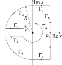
Figure 1: Contour $\Gamma.$

The integrals along contours $\Gamma_{3}$ (parametrized by $s=\rho\mathrm{e}^{\mathrm{i}\pi},$ $\rho\in\left(r,R\right)$) and $\Gamma_{5}$ (parametrized by $s=\rho\mathrm{e}^{-\mathrm{i}\pi},$ $\rho\in\left(r,R\right)$) in the case of relaxation modulus (32) read

$$\lim_{\begin{subarray}{c}R\rightarrow\infty,\\ r\rightarrow 0\end{subarray}}\int_{\Gamma_{3}}\tilde{\sigma}_{sr}\left(s\right)\mathrm{e}^{st}\mathrm{d}s = \int_{\infty}^{0}\frac{1}{\rho\mathrm{e}^{\mathrm{i}\pi}}\frac{\Phi_{\varepsilon}\left(\rho\mathrm{e}^{\mathrm{i}\pi}\right)}{\Phi_{\sigma}\left(\rho\mathrm{e}^{\mathrm{i}\pi}\right)}\mathrm{e}^{-\rho t}\mathrm{e}^{\mathrm{i}\pi}\mathrm{d}\rho=-\int_{0}^{\infty}\frac{\Phi_{\varepsilon}\left(\rho\mathrm{e}^{\mathrm{i}\pi}\right)}{\Phi_{\sigma}\left(\rho\mathrm{e}^{\mathrm{i}\pi}\right)}\frac{\mathrm{e}^{-\rho t}}{\rho}\mathrm{d}\rho,$$

$$\lim_{\begin{subarray}{c}R\rightarrow\infty,\\ r\rightarrow 0\end{subarray}}\int_{\Gamma_{5}}\tilde{\sigma}_{sr}\left(s\right)\mathrm{e}^{st}\mathrm{d}s = \int_{0}^{\infty}\frac{1}{\rho\mathrm{e}^{-\mathrm{i}\pi}}\frac{\Phi_{\varepsilon}\left(\rho\mathrm{e}^{-\mathrm{i}\pi}\right)}{\Phi_{\sigma}\left(\rho\mathrm{e}^{-\mathrm{i}\pi}\right)}\mathrm{e}^{-\rho t}\mathrm{e}^{-\mathrm{i}\pi}\mathrm{d}\rho=\int_{0}^{\infty}\frac{\bar{\Phi}_{\varepsilon}\left(\rho\mathrm{e}^{\mathrm{i}\pi}\right)}{\bar{\Phi}_{\sigma}\left(\rho\mathrm{e}^{\mathrm{i}\pi}\right)}\frac{\mathrm{e}^{-\rho t}}{\rho}\mathrm{d}\rho,$$

while for the creep compliance in the form (35), the integrals are

$$\lim_{\begin{subarray}{c}R\rightarrow\infty,\\ r\rightarrow 0\end{subarray}}\int_{\Gamma_{3}}\tilde{\varepsilon}_{cr}\left(s\right)\mathrm{e}^{st}\mathrm{d}s = \int_{\infty}^{0}\frac{1}{\rho\mathrm{e}^{\mathrm{i}\pi}}\frac{\Phi_{\sigma}\left(\rho\mathrm{e}^{\mathrm{i}\pi}\right)}{\Phi_{\varepsilon}\left(\rho\mathrm{e}^{\mathrm{i}\pi}\right)}\mathrm{e}^{-\rho t}\mathrm{e}^{\mathrm{i}\pi}\mathrm{d}\rho=-\int_{0}^{\infty}\frac{\Phi_{\sigma}\left(\rho\mathrm{e}^{\mathrm{i}\pi}\right)}{\Phi_{\varepsilon}\left(\rho\mathrm{e}^{\mathrm{i}\pi}\right)}\frac{\mathrm{e}^{-\rho t}}{\rho}\mathrm{d}\rho,$$

$$\lim_{\begin{subarray}{c}R\rightarrow\infty,\\ r\rightarrow 0\end{subarray}}\int_{\Gamma_{5}}\tilde{\varepsilon}_{cr}\left(s\right)\mathrm{e}^{st}\mathrm{d}s = \int_{0}^{\infty}\frac{1}{\rho\mathrm{e}^{-\mathrm{i}\pi}}\frac{\Phi_{\sigma}\left(\rho\mathrm{e}^{-\mathrm{i}\pi}\right)}{\Phi_{\varepsilon}\left(\rho\mathrm{e}^{-\mathrm{i}\pi}\right)}\mathrm{e}^{-\rho t}\mathrm{e}^{-\mathrm{i}\pi}\mathrm{d}\rho=\int_{0}^{\infty}\frac{\bar{\Phi}_{\sigma}\left(\rho\mathrm{e}^{\mathrm{i}\pi}\right)}{\bar{\Phi}_{\varepsilon}\left(\rho\mathrm{e}^{\mathrm{i}\pi}\right)}\frac{\mathrm{e}^{-\rho t}}{\rho}\mathrm{d}\rho,$$

and for the creep compliance in the form (37) their form is

$$\lim_{\begin{subarray}{c}R\rightarrow\infty,\\ r\rightarrow 0\end{subarray}}\int_{\Gamma_{3}}\tilde{f}_{cr}\left(s\right)\mathrm{e}^{st}\mathrm{d}s = \int_{\infty}^{0}\frac{\Phi_{\sigma}\left(\rho\mathrm{e}^{\mathrm{i}\pi}\right)}{\Phi_{\varepsilon}\left(\rho\mathrm{e}^{\mathrm{i}\pi}\right)}\mathrm{e}^{-\rho t}\mathrm{e}^{\mathrm{i}\pi}\mathrm{d}\rho=\int_{0}^{\infty}\frac{\Phi_{\sigma}\left(\rho\mathrm{e}^{\mathrm{i}\pi}\right)}{\Phi_{\varepsilon}\left(\rho\mathrm{e}^{\mathrm{i}\pi}\right)}\mathrm{e}^{-\rho t}\mathrm{d}\rho,$$

$$\lim_{\begin{subarray}{c}R\rightarrow\infty,\\ r\rightarrow 0\end{subarray}}\int_{\Gamma_{5}}\tilde{f}_{cr}\left(s\right)\mathrm{e}^{st}\mathrm{d}s = \int_{0}^{\infty}\frac{\Phi_{\sigma}\left(\rho\mathrm{e}^{-\mathrm{i}\pi}\right)}{\Phi_{\varepsilon}\left(\rho\mathrm{e}^{-\mathrm{i}\pi}\right)}\mathrm{e}^{-\rho t}\mathrm{e}^{-\mathrm{i}\pi}\mathrm{d}\rho=-\int_{0}^{\infty}\frac{\bar{\Phi}_{\sigma}\left(\rho\mathrm{e}^{\mathrm{i}\pi}\right)}{\bar{\Phi}_{\varepsilon}\left(\rho\mathrm{e}^{\mathrm{i}\pi}\right)}\mathrm{e}^{-\rho t}\mathrm{d}\rho,$$

where, according to (17), one has $\Phi_{\sigma}\left(\bar{s}\right)=\bar{\Phi}_{\sigma}\left(s\right)$ and $\Phi_{\varepsilon}\left(\bar{s}\right)=\bar{\Phi}_{\varepsilon}\left(s\right)$ (bar denotes the complex conjugation), so that

$$\lim_{\begin{subarray}{c}R\rightarrow\infty,\\ r\rightarrow 0\end{subarray}}\int_{\Gamma_{3}\cup\Gamma_{5}}\tilde{\sigma}_{sr}\left(s\right)\mathrm{e}^{st}\mathrm{d}s = \int_{0}^{\infty}\left(\frac{\bar{\Phi}_{\varepsilon}\left(\rho\mathrm{e}^{\mathrm{i}\pi}\right)}{\bar{\Phi}_{\sigma}\left(\rho\mathrm{e}^{\mathrm{i}\pi}\right)}-\frac{\Phi_{\varepsilon}\left(\rho\mathrm{e}^{\mathrm{i}\pi}\right)}{\Phi_{\sigma}\left(\rho\mathrm{e}^{\mathrm{i}\pi}\right)}\right)\frac{\mathrm{e}^{-\rho t}}{\rho}\mathrm{d}\rho=-2\mathrm{i}\int_{0}^{\infty}\frac{K\left(\rho\right)}{\left|\Phi_{\sigma}\left(\rho\mathrm{e}^{\mathrm{i}\pi}\right)\right|^{2}}\frac{\mathrm{e}^{-\rho t}}{\rho}\mathrm{d}\rho,$$ (80)

$$\lim_{\begin{subarray}{c}R\rightarrow\infty,\\ r\rightarrow 0\end{subarray}}\int_{\Gamma_{3}\cup\Gamma_{5}}\tilde{\varepsilon}_{cr}\left(s\right)\mathrm{e}^{st}\mathrm{d}s = \int_{0}^{\infty}\left(\frac{\bar{\Phi}_{\sigma}\left(\rho\mathrm{e}^{\mathrm{i}\pi}\right)}{\bar{\Phi}_{\varepsilon}\left(\rho\mathrm{e}^{\mathrm{i}\pi}\right)}-\frac{\Phi_{\sigma}\left(\rho\mathrm{e}^{\mathrm{i}\pi}\right)}{\Phi_{\varepsilon}\left(\rho\mathrm{e}^{\mathrm{i}\pi}\right)}\right)\frac{\mathrm{e}^{-\rho t}}{\rho}\mathrm{d}\rho=2\mathrm{i}\int_{0}^{\infty}\frac{K\left(\rho\right)}{\left|\Phi_{\varepsilon}\left(\rho\mathrm{e}^{\mathrm{i}\pi}\right)\right|^{2}}\frac{\mathrm{e}^{-\rho t}}{\rho}\mathrm{d}\rho,$$ (81)

$$\lim_{\begin{subarray}{c}R\rightarrow\infty,\\ r\rightarrow 0\end{subarray}}\int_{\Gamma_{3}\cup\Gamma_{5}}\tilde{f}_{cr}\left(s\right)\mathrm{e}^{st}\mathrm{d}s = \int_{0}^{\infty}\left(\frac{\Phi_{\sigma}\left(\rho\mathrm{e}^{\mathrm{i}\pi}\right)}{\Phi_{\varepsilon}\left(\rho\mathrm{e}^{\mathrm{i}\pi}\right)}-\frac{\bar{\Phi}_{\sigma}\left(\rho\mathrm{e}^{\mathrm{i}\pi}\right)}{\bar{\Phi}_{\varepsilon}\left(\rho\mathrm{e}^{\mathrm{i}\pi}\right)}\right)\mathrm{e}^{-\rho t}\mathrm{d}\rho=-2\mathrm{i}\int_{0}^{\infty}\frac{K\left(\rho\right)}{\left|\Phi_{\varepsilon}\left(\rho\mathrm{e}^{\mathrm{i}\pi}\right)\right|^{2}}\mathrm{e}^{-\rho t}\mathrm{d}\rho,$$ (82)

respectively, with

$$K\left(\rho\right)=\frac{1}{2\mathrm{i}}\left(\bar{\Phi}_{\sigma}\left(\rho\mathrm{e}^{\mathrm{i}\pi}\right)\Phi_{\varepsilon}\left(\rho\mathrm{e}^{\mathrm{i}\pi}\right)-\Phi_{\sigma}\left(\rho\mathrm{e}^{\mathrm{i}\pi}\right)\bar{\Phi}_{\varepsilon}\left(\rho\mathrm{e}^{\mathrm{i}\pi}\right)\right)$$

giving (34). According to the Cauchy integral theorem (79), the integrals (80) and (81) yield the second terms in relaxation modulus (32) and creep compliance (35), while the integral (82) yields function $f_{cr}$ in (78), since the integrals along $\Gamma_{1},$ $\Gamma_{2},$ $\Gamma_{6},$ $\Gamma_{7}$ tend to zero as $R\rightarrow\infty$ and $r\rightarrow 0,$ and the integral along $\Gamma_{4}$ is: nonzero in cases of (32) and (35), and zero in the case of (78).

The contour $\Gamma_{1}$ is parametrized by $s=p+iR,$ $p\in\left(0,p_{0}\right),$ with $R\rightarrow\infty,$ so that the integrals

$$\int_{\Gamma_{1}}\tilde{\sigma}_{sr}\left(s\right)\mathrm{e}^{st}\mathrm{d}s = \int_{p_{0}}^{0}\frac{1}{p+\mathrm{i}R}\frac{\Phi_{\varepsilon}\left(p+\mathrm{i}R\right)}{\Phi_{\sigma}(p+\mathrm{i}R)}\mathrm{e}^{\left(p+\mathrm{i}R\right)t}\mathrm{d}p,$$

$$\int_{\Gamma_{1}}\tilde{\varepsilon}_{cr}\left(s\right)\mathrm{e}^{st}\mathrm{d}s = \int_{p_{0}}^{0}\frac{1}{p+\mathrm{i}R}\frac{\Phi_{\sigma}\left(p+\mathrm{i}R\right)}{\Phi_{\varepsilon}(p+\mathrm{i}R)}\mathrm{e}^{\left(p+\mathrm{i}R\right)t}\mathrm{d}p,$$

$$\int_{\Gamma_{1}}\tilde{f}_{cr}\left(s\right)\mathrm{e}^{st}\mathrm{d}s = \int_{p_{0}}^{0}\frac{\Phi_{\sigma}\left(p+\mathrm{i}R\right)}{\Phi_{\varepsilon}(p+\mathrm{i}R)}\mathrm{e}^{\left(p+\mathrm{i}R\right)t}\mathrm{d}p$$

are estimated as

$$\left|\int_{\Gamma_{1}}\tilde{\sigma}_{sr}\left(s\right)\mathrm{e}^{st}\mathrm{d}s\right| \leq \int_{0}^{p_{0}}\frac{1}{\left|p+\mathrm{i}R\right|}\left|\frac{\Phi_{\varepsilon}\left(p+\mathrm{i}R\right)}{\Phi_{\sigma}(p+\mathrm{i}R)}\right|\mathrm{e}^{pt}\mathrm{d}p,$$

$$\left|\int_{\Gamma_{1}}\tilde{\varepsilon}_{cr}\left(s\right)\mathrm{e}^{st}\mathrm{d}s\right| \leq \int_{0}^{p_{0}}\frac{1}{\left|p+\mathrm{i}R\right|}\left|\frac{\Phi_{\sigma}\left(p+\mathrm{i}R\right)}{\Phi_{\varepsilon}(p+\mathrm{i}R)}\right|\mathrm{e}^{pt}\mathrm{d}p,$$

$$\left|\int_{\Gamma_{1}}\tilde{f}_{cr}\left(s\right)\mathrm{e}^{st}\mathrm{d}s\right| \leq \int_{0}^{p_{0}}\left|\frac{\Phi_{\sigma}\left(p+\mathrm{i}R\right)}{\Phi_{\varepsilon}(p+\mathrm{i}R)}\right|\mathrm{e}^{pt}\mathrm{d}p.$$

Assuming $s=\rho e^{\mathrm{i}\varphi},$ since $R\rightarrow\infty,$ one obtains $\rho=\sqrt{p^{2}+R^{2}}\sim R$ and $\varphi=\arctan\frac{R}{p}\sim\frac{\pi}{2},$ the previous expressions become

$$\lim_{R\rightarrow\infty}\left|\int_{\Gamma_{1}}\tilde{\sigma}_{sr}\left(s\right)\mathrm{e}^{st}\mathrm{d}s\right| \leq \lim_{R\rightarrow\infty}\int_{0}^{p_{0}}\frac{1}{R}\left|\frac{\Phi_{\varepsilon}\left(R\mathrm{e}^{\mathrm{i}\frac{\pi}{2}}\right)}{\Phi_{\sigma}(R\mathrm{e}^{\mathrm{i}\frac{\pi}{2}})}\right|\mathrm{e}^{pt}\mathrm{d}p=0,$$

$$\lim_{R\rightarrow\infty}\left|\int_{\Gamma_{1}}\tilde{\varepsilon}_{cr}\left(s\right)\mathrm{e}^{st}\mathrm{d}s\right| \leq \lim_{R\rightarrow\infty}\int_{0}^{p_{0}}\frac{1}{R}\left|\frac{\Phi_{\sigma}\left(R\mathrm{e}^{\mathrm{i}\frac{\pi}{2}}\right)}{\Phi_{\varepsilon}(R\mathrm{e}^{\mathrm{i}\frac{\pi}{2}})}\right|\mathrm{e}^{pt}\mathrm{d}p=0,$$

$$\lim_{R\rightarrow\infty}\left|\int_{\Gamma_{1}}\tilde{f}_{cr}\left(s\right)\mathrm{e}^{st}\mathrm{d}s\right| \leq \lim_{R\rightarrow\infty}\int_{0}^{p_{0}}\left|\frac{\Phi_{\sigma}\left(R\mathrm{e}^{\mathrm{i}\frac{\pi}{2}}\right)}{\Phi_{\varepsilon}(R\mathrm{e}^{\mathrm{i}\frac{\pi}{2}})}\right|\mathrm{e}^{pt}\mathrm{d}p=0,$$

due to assumptions $\left(A2\right),$ $\left(A3\right),$ and $\left(A4\right),$ respectively. Analogously, it can be proved that the integral along $\Gamma_{7}$ tends to zero as well.

The integrals along contour $\Gamma_{2},$ parametrized by $s=R\mathrm{e}^{\mathrm{i}\varphi},$ $\varphi\in\left(\frac{\pi}{2},\pi\right),$ with $R\rightarrow\infty,$ are

$$\int_{\Gamma_{2}}\tilde{\sigma}_{sr}\left(s\right)\mathrm{e}^{st}\mathrm{d}s = \int_{\frac{\pi}{2}}^{\pi}\frac{1}{R\mathrm{e}^{\mathrm{i}\varphi}}\frac{\Phi_{\varepsilon}(R\mathrm{e}^{\mathrm{i}\varphi})}{\Phi_{\sigma}(R\mathrm{e}^{\mathrm{i}\varphi})}\mathrm{e}^{Rt\mathrm{e}^{\mathrm{i}\varphi}}\mathrm{i}R\mathrm{e}^{\mathrm{i}\varphi}\mathrm{d}\varphi,$$

$$\int_{\Gamma_{2}}\tilde{\varepsilon}_{cr}\left(s\right)\mathrm{e}^{st}\mathrm{d}s = \int_{\frac{\pi}{2}}^{\pi}\frac{1}{R\mathrm{e}^{\mathrm{i}\varphi}}\frac{\Phi_{\sigma}(R\mathrm{e}^{\mathrm{i}\varphi})}{\Phi_{\varepsilon}(R\mathrm{e}^{\mathrm{i}\varphi})}\mathrm{e}^{Rt\mathrm{e}^{\mathrm{i}\varphi}}\mathrm{i}R\mathrm{e}^{\mathrm{i}\varphi}\mathrm{d}\varphi,$$

$$\int_{\Gamma_{2}}\tilde{f}_{cr}\left(s\right)\mathrm{e}^{st}\mathrm{d}s = \int_{\frac{\pi}{2}}^{\pi}\frac{\Phi_{\sigma}(R\mathrm{e}^{\mathrm{i}\varphi})}{\Phi_{\varepsilon}(R\mathrm{e}^{\mathrm{i}\varphi})}\mathrm{e}^{Rt\mathrm{e}^{\mathrm{i}\varphi}}\mathrm{i}R\mathrm{e}^{\mathrm{i}\varphi}\mathrm{d}\varphi$$

respectively, yielding the estimates

$$\left|\int_{\Gamma_{2}}\tilde{\sigma}_{sr}\left(s\right)\mathrm{e}^{st}\mathrm{d}s\right| \leq \int_{\frac{\pi}{2}}^{\pi}\left|\frac{\Phi_{\varepsilon}(R\mathrm{e}^{\mathrm{i}\varphi})}{\Phi_{\sigma}(R\mathrm{e}^{\mathrm{i}\varphi})}\right|\mathrm{e}^{Rt\cos\varphi}\mathrm{d}\varphi=0,$$

$$\left|\int_{\Gamma_{2}}\tilde{\varepsilon}_{cr}\left(s\right)\mathrm{e}^{st}\mathrm{d}s\right| \leq \int_{\frac{\pi}{2}}^{\pi}\left|\frac{\Phi_{\sigma}(R\mathrm{e}^{\mathrm{i}\varphi})}{\Phi_{\varepsilon}(R\mathrm{e}^{\mathrm{i}\varphi})}\right|\mathrm{e}^{Rt\cos\varphi}\mathrm{d}\varphi=0,$$

$$\left|\int_{\Gamma_{2}}\tilde{f}_{cr}\left(s\right)\mathrm{e}^{st}\mathrm{d}s\right| \leq \int_{\frac{\pi}{2}}^{\pi}R\left|\frac{\Phi_{\sigma}(R\mathrm{e}^{\mathrm{i}\varphi})}{\Phi_{\varepsilon}(R\mathrm{e}^{\mathrm{i}\varphi})}\right|\mathrm{e}^{Rt\cos\varphi}\mathrm{d}\varphi=0.$$

due to assumptions $\left(A2\right),$ $\left(A3\right),$ and $\left(A4\right),$ respectively. By the similar arguments, the integral along $\Gamma_{6}$ tends to zero as well.

Parametrization of the contour $\Gamma_{4}$ is $s=r\mathrm{e}^{\mathrm{i}\varphi},$ $\varphi\in\left(-\pi,\pi\right),$ with $r\rightarrow 0,$ so that

$$\int_{\Gamma_{4}}\tilde{\sigma}_{sr}\left(s\right)\mathrm{e}^{st}\mathrm{d}s = \int_{\pi}^{-\pi}\frac{1}{r\mathrm{e}^{\mathrm{i}\varphi}}\frac{\Phi_{\varepsilon}(r\mathrm{e}^{\mathrm{i}\varphi})}{\Phi_{\sigma}(r\mathrm{e}^{\mathrm{i}\varphi})}\mathrm{e}^{rt\mathrm{e}^{\mathrm{i}\varphi}}\mathrm{i}r\mathrm{e}^{\mathrm{i}\varphi}\mathrm{d}\varphi,$$

$$\int_{\Gamma_{4}}\tilde{\varepsilon}_{cr}\left(s\right)\mathrm{e}^{st}\mathrm{d}s = \int_{\pi}^{-\pi}\frac{1}{r\mathrm{e}^{\mathrm{i}\varphi}}\frac{\Phi_{\sigma}(r\mathrm{e}^{\mathrm{i}\varphi})}{\Phi_{\varepsilon}(r\mathrm{e}^{\mathrm{i}\varphi})}\mathrm{e}^{rt\mathrm{e}^{\mathrm{i}\varphi}}\mathrm{i}r\mathrm{e}^{\mathrm{i}\varphi}\mathrm{d}\varphi,$$

$$\int_{\Gamma_{4}}\tilde{f}_{cr}\left(s\right)\mathrm{e}^{st}\mathrm{d}s = \int_{\pi}^{-\pi}\frac{\Phi_{\sigma}(r\mathrm{e}^{\mathrm{i}\varphi})}{\Phi_{\varepsilon}(r\mathrm{e}^{\mathrm{i}\varphi})}\mathrm{e}^{rt\mathrm{e}^{\mathrm{i}\varphi}}\mathrm{i}r\mathrm{e}^{\mathrm{i}\varphi}\mathrm{d}\varphi$$

respectively, yield

$$\lim_{r\rightarrow 0}\int_{\Gamma_{4}}\tilde{\sigma}_{sr}\left(s\right)\mathrm{e}^{st}\mathrm{d}s = -\mathrm{i\,}\lim_{r\rightarrow 0}\int_{-\pi}^{\pi}\frac{\Phi_{\varepsilon}(r\mathrm{e}^{\mathrm{i}\varphi})}{\Phi_{\sigma}(r\mathrm{e}^{\mathrm{i}\varphi})}\mathrm{d}\varphi=-2\pi\mathrm{i}\sigma_{sr}^{\left(e\right)},$$

$$\lim_{r\rightarrow 0}\int_{\Gamma_{4}}\tilde{\varepsilon}_{cr}\left(s\right)\mathrm{e}^{st}\mathrm{d}s = -\mathrm{i\,}\lim_{r\rightarrow 0}\int_{-\pi}^{\pi}\frac{\Phi_{\sigma}(r\mathrm{e}^{\mathrm{i}\varphi})}{\Phi_{\varepsilon}(r\mathrm{e}^{\mathrm{i}\varphi})}\mathrm{d}\varphi=-2\pi\mathrm{i}\varepsilon_{cr}^{\left(e\right)},$$

$$\lim_{r\rightarrow 0}\left|\int_{\Gamma_{4}}\tilde{f}_{cr}\left(s\right)\mathrm{e}^{st}\mathrm{d}s\right| \leq \lim_{r\rightarrow 0}\int_{-\pi}^{\pi}r\left|\frac{\Phi_{\sigma}(r\mathrm{e}^{\mathrm{i}\varphi})}{\Phi_{\varepsilon}(r\mathrm{e}^{\mathrm{i}\varphi})}\right|\mathrm{d}\varphi=0,$$

due to (33), (36), and assumption $\left(A4\right).$

References

• [1] T. M. Atanackovic. On a distributed derivative model of a viscoelastic body. Comptes Rendus Mécanique, 331:687–692, 2003.
• [2] T. M. Atanackovic, M. Janev, Lj. Oparnica, S. Pilipovic, and D. Zorica. Space-time fractional Zener wave equation. Proceedings of the Royal Society A: Mathematical, Physical and Engineering Sciences, 471:20140614–1–25, 2015.
• [3] T. M. Atanackovic, S. Konjik, Lj. Oparnica, and D. Zorica. Thermodynamical restrictions and wave propagation for a class of fractional order viscoelastic rods. Abstract and Applied Analysis, 2011:ID975694–1–32, 2011.
• [4] T. M. Atanackovic, S. Pilipovic, B. Stankovic, and D. Zorica. Fractional Calculus with Applications in Mechanics: Wave Propagation, Impact and Variational Principles. Wiley-ISTE, London, 2014.
• [5] T. M. Atanackovic and B. Stankovic. Generalized wave equation in nonlocal elasticity. Acta Mechanica, 208:1–10, 2009.
• [6] P. W. Buchen and F. Mainardi. Asymptotic expansions for transient viscoelastic waves. Journal de mécanique, 14:597–608, 1975.
• [7] W. Cai, W. Chen, J. Fang, and S. Holm. A survey on fractional derivative modeling of power-law frequency-dependent viscous dissipative and scattering attenuation in acoustic wave propagation. Applied Mechanics Reviews, 70:1–12, 2018.
• [8] S. Carillo. Singular kernel problems in materials with memory. Meccanica, 50:603–615, 2015.
• [9] S. Carillo. A 3-dimensional singular kernel problem in viscoelasticity: An existence result. AAPP Atti della Accademia Peloritana dei Pericolanti, Classe di Scienze Fisiche, Matematiche e Naturali, 97(S1):A3–1–A3–13, 2019.
• [10] S. Carillo, M. Chipot, V. Valente, and G. V. Caffarelli. On weak regularity requirements of the relaxation modulus in viscoelasticity. Communications in Applied and Industrial Mathematics, 10:78–87, 2019.
• [11] N. Challamel, D. Zorica, T. M. Atanacković, and D. T. Spasić. On the fractional generalization of Eringen’s nonlocal elasticity for wave propagation. Comptes Rendus Mécanique, 341:298–303, 2013.
• [12] I. Colombaro, A. Giusti, and F. Mainardi. On transient waves in linear viscoelasticity. Wave Motion, 74:191–212, 2017.
• [13] A. Evgrafov and J. C. Bellido. From non-local Eringen’s model to fractional elasticity. Mathematics and Mechanics of Solids, 24:1935–1953, 2019.
• [14] A. Hanyga. Wave propagation in linear viscoelastic media with completely monotonic relaxation moduli. Wave Motion, 50:909–928, 2013.
• [15] A. Hanyga. Attenuation and shock waves in linear hereditary viscoelastic media; Strick-Mainardi, Jeffreys-Lomnitz-Strick and Andrade creep compliances. Pure and Applied Geophysics, 171:2097–2109, 2014.
• [16] A. Hanyga. Dispersion and attenuation for an acoustic wave equation consistent with viscoelasticity. Journal of Computational Acoustics, 22:1450006–1–22, 2014.
• [17] A. Hanyga. Asymptotic estimates of viscoelastic Green’s functions near the wavefront. Quarterly of Applied Mathematics, 73:679–692, 2015.
• [18] A. Hanyga. Effects of Newtonian viscosity and relaxation on linear viscoelastic wave propagation. Archive of Applied Mechanics, 2019.
• [19] A. Hanyga and M. Seredyńska. Positivity of Green’s functions for a class of partial integro-differential equations including viscoelasticity. Wave Motion, 47:648–662, 2010.
• [20] S. Holm. Waves with Power-Law Attenuation. Springer Nature Switzerland AG, Cham, 2019.
• [21] G. Hörmann, Lj. Oparnica, and D. Zorica. Microlocal analysis of fractional wave equations. Zeitschrift für angewandte Mathematik und Mechanik, 97:217–225, 2017.
• [22] G. Hörmann, Lj. Oparnica, and D. Zorica. Solvability and microlocal analysis of the fractional Eringen wave equation. Mathematics and Mechanics of Solids, 23:1420–1430, 2018.
• [23] A. A. Kilbas, H. M. Srivastava, and J. J. Trujillo. Theory and Applications of Fractional Differential Equations. Elsevier B.V., Amsterdam, 2006.
• [24] S. Konjik, Lj. Oparnica, and D. Zorica. Waves in fractional Zener type viscoelastic media. Journal of Mathematical Analysis and Applications, 365:259–268, 2010.
• [25] S. Konjik, Lj. Oparnica, and D. Zorica. Waves in viscoelastic media described by a linear fractional model. Integral Transforms and Special Functions, 22:283–291, 2011.
• [26] S. Konjik, Lj. Oparnica, and D. Zorica. Distributed-order fractional constitutive stress-strain relation in wave propagation modeling. Zeitschrift für angewandte Mathematik und Physik, 70:51–1–21, 2019.
• [27] F. Mainardi. Fractional Calculus and Waves in Linear Viscoelasticity. Imperial College Press, London, 2010.
• [28] N. Makris. The frequency response function of the creep compliance. Meccanica, 54:19–31, 2019.
• [29] A. O. Malkhanov, V. I. Erofeev, and A. V. Leontieva. Nonlinear travelling strain waves in a gradient-elastic medium. Continuum Mechanics and Thermodynamics, 31:1931–1940, 2019.
• [30] A. S. Okuka and D. Zorica. Formulation of thermodynamically consistent fractional Burgers models. Acta Mechanica, 229:3557–3570, 2018.
• [31] A. S. Okuka and D. Zorica. Fractional Burgers models in creep and stress relaxation tests. Applied Mathematical Modelling, 77:1894–1935, 2020.
• [32] Lj. Oparnica and E. Süli. Well-posedness of the fractional Zener wave equation for heterogenous viscoelastic materials. Fractional Calculus and Applied Analysis, 2020.
• [33] Lj. Oparnica, D. Zorica, and A. S. Okuka. Fractional Burgers wave equation. Acta Mechanica, 230:4321–4340, 2019.
• [34] F. Saedpanah. Well-posedness of an integro-differential equation with positive type kernels modeling fractional order viscoelasticity. European Journal of Mechanics A/Solids, 44:201–211, 2014.
• [35] S. A. Silling. Attenuation of waves in a viscoelastic peridynamic medium. Mathematics and Mechanics of Solids, 24:3597–3613, 2019.
• [36] K. Šiškova. Inverse source problems in evolutionary PDE’s. PhD thesis, Ghent University, Ghent, 2018. https://biblio.ugent.be/publication/8583819/file/8583821.pdf.
• [37] Y. Wang and Y. Wang. Exponential energy decay of solutions of viscoelastic wave equations. Journal of Mathematical Analysis and Applications, 347:18–25, 2008.
• [38] B. Wu. On seismic wave propagation through subsurface media. European Physical Journal Plus, 134:357–1–8, 2019.
• [39] R. Zacher. Boundedness of weak solutions to evolutionary partial integro-differential equations with discontinuous coefficients. Journal of Mathematical Analysis and Applications, 348:137–149, 2008.