Speeding up Word Mover’s Distance and its variants via properties of distances between embeddings

Abstract

The Word Mover’s Distance (WMD) proposed by Kusner et al. is a distance between documents that takes advantage of semantic relations among words that are captured by their embeddings. This distance proved to be quite effective, obtaining state-of-art error rates for classification tasks, but is also impracticable for large collections/documents due to its computational complexity. For circumventing this problem, variants of WMD have been proposed. Among them, Relaxed Word Mover’s Distance (RWMD) is one of the most successful due to its simplicity, effectiveness, and also because of its fast implementations.

Relying on assumptions that are supported by empirical properties of the distances between embeddings, we propose an approach to speed up both WMD and RWMD. Experiments over 10 datasets suggest that our approach leads to a significant speed-up in document classification tasks while maintaining the same error rates.

1 INTRODUCTION

Document comparison is a fundamental step in several applications such as recommendation, clustering, search, and categorization. In its simplest version, this task consists of computing the distance between a single pair of documents.

The document representation is an essential factor in the definition of a distance. Arguably, the most employed document representations due to its simplicity and good results are the Bag-of-Words (BOW) and the Term Frequency - Inverse Document Frequency (TF-IDF). These representations are based on word counts, and so they may lose information that is relevant for some applications, such as the ordering among words in a document, co-occurrence, and semantic relations between different words. Thus, richer representations that take into account some of this information have been proposed [24, 8, 4].

Up to a few years ago, semantic relations were barely used because there was no adequate methodology of how to obtain them. Consequently, researchers eventually decided to use ontologies as a way to mitigate this issue [12], although this makes applications dependent on an external knowledge base. This scenario changed with the emergence of Word2Vec [17, 18] and its variants [20], a class of methods that allow us to efficiently identify the relationship between words and embed them into vectors, called word embeddings. As a result, researchers have been searching for ways to use these embeddings to refine existing models in the literature. The results of these efforts can already be seen in works such as [15, 14, 7, 16], and indeed, improvements are obtained.

In particular, Kusner et al. [14] propose the Word Mover’s Distance (WMD), an application of the classic Earth Mover’s Distance (EMD) [23] for the domain of documents that takes advantage of the semantic relations captured by the embeddings associated with their words. The idea is to compute the minimum cost required to transform one document representation into another by using the distance between embeddings as the cost of transforming words. In fact, the distance is given by the cost of an optimal solution of a transportation problem defined on a complete bipartite graph where the nodes correspond to the distinct words of the documents, and the edge costs are the distance between embeddings. In the same paper, they show that this approach obtained outstanding results on document classification tasks, outperforming many competitors. The major drawback of WMD, however, is its high computational cost since solving the transportation problem in a complete bipartite graph is costly, requiring super cubic time.

Since the proposal of WMD, there has been a considerable amount of research focusing on improving its performance while keeping its effectiveness [14, 3, 25, 2]. The Relaxed Word Mover’s Distance (RWMD) [14, 3, 2], due to its simplicity and speed, is arguably one of the most successful outcomes of this research effort. In fact, experiments reported in the literature show that it achieves quality (test error) competitive with those obtained by WMD with the advantage of being much faster. However, despite its good performance, further improvements are relevant because there are applications in which this kind of distance needs to be calculated very quickly.

Motivated by this scenario, we focus on developing an approach to derive distances that are as effective as WMD and its variants with the advantage of allowing a faster computation.

1.1 Our Contributions

To achieve this goal, in contrast to other approaches available, we explore the properties of the application domain, more specifically the distribution of distances among word embeddings. Our key observation is that one can assume, without incurring a significant loss, that the set of distances between word embeddings is split into two sets: the set of distances between related words and the set of distances between non-related words, with the distances in the latter having the same value. We show that this assumption, which is supported by empirical data, can be used to: (i) obtain a more compact formulation for the transportation problem that is used to calculate WMD and its variants and (ii) dramatically reduce the memory required to cache the distances between embeddings, which is essential for the fast computation of RWMD for large vocabularies since the evaluation of the distance between a pair of words requires hundreds of operations for typical sizes of embeddings.

By relying on the previous observation, we propose a simple approach for speeding up WMD and distances with a similar flavour. More concretely, we show how to derive new distances between documents by applying our approach to both WMD and RWMD. The time and space complexities required to compute these distances depend on a parameter $r$ that has to do with the number of related words. This parameter can be set to a small value which leads to complexity improvements over WMD and RWMD. In addition, experiments executed over 10 datasets, for two distinct tasks, suggest that these distances yield to test errors as good as those obtained by WMD/RWMD, with a significant gain in terms of execution time. Indeed, with regards to efficient implementations of RWMD, we obtained an average speed-up of almost 5 times for one task and 15 times for the other.

1.2 Related Work

Our work is closely related to some approaches that have been proposed to circumvent the high computational cost of WMD [14, 3, 25, 2].

Kusner et al. [14] propose the Relaxed Word Mover’s Distance (RWMD), a distance that is defined over a relaxation of the transportation problem in which some constraints are dropped. Given the distance matrix between the words embeddings of documents $D$ and $D^{\prime}$, the RWMD can be calculated in $O(|D|\cdot|D^{\prime}|)$ time, where $|D|$ and $|D^{\prime}|$ are the number of distinct words of $D$ and $D^{\prime}$, respectively. Thus, the bottleneck of RWMD is to compute the distance matrix which costs $O(|D|\cdot|D^{\prime}|\cdot d)$ time, where $d$ is the dimension of the word embeddings space. Such cost can be prevented by caching the $O(n^{2})$ distances between all the $n$ words of the vocabulary, an approach that could be prohibitive for large $n$. Experiments from [14] shows that RWMD achieves test error competitive with WMD for document classification tasks while incurring a lower computational cost, even without using cache.

Atasu et al. [3] show how to compute RWMD for any two documents $D$ and $D^{\prime}$ from a collection ${\cal C}$ in $O(|D|+|D^{\prime}|)$ time. To achieve this running time, they need to pre-compute and store the distance of word $w$ to the nearest word in document $D$, for each $w$ in the vocabulary and each $D$ in the collection. Thus, it consumes $O(n|{\cal C}|)$ memory, where $|{\cal C}|$ is the number of documents in ${\cal C}$, which may be infeasible for large collections. Furthermore, this linear time complexity does not hold for dynamic collections since the method requires $O(|D^{new}|\cdot n\cdot d)$ preprocessing time before calculating the RWMD from a new document $D^{new}$ to some document $D$. Further work from Atasu et al. [2] discusses a limitation of RWMD for documents that share many words and then proposes a family of variants of RWMD that better address this scenario.

In a broader scope, our work is also related to some proposals to speed up EMD [19] and approximate solutions for transportation problems in general [5, 9, 22].

Pele et al. [19] present an optimized solution of the EMD for instances in which the costs of the edges satisfies certain properties that are motivated by the way human perceive distances. The optimization introduced by this approach consists of reducing the number of edges in the transportation network and, as a consequence, the running time. This work resembles ours in the sense that both optimize the time complexity to solve the transportation problem by taking into account how the costs behave in the domains under consideration.

Cuturi et al. [5] use an entropic regularization term to smooth out the transportation problem so that it can be solved much faster via Sinkhorn’s matrix scaling algorithm. This algorithm has $O(|D|\cdot|D^{\prime}|)$ empirical time according to [5] and it was used in a supervised version of WMD [13]. As RWMD, this method needs an $O(n^{2})$ space cache in order to prevent the $O(|D|\cdot|D^{\prime}|\cdot d)$ time required to compute the distances between the words in $D$ and $D^{\prime}$.

1.3 Paper Organization

The paper is organized as follows. In Section 2, we introduce our notation and discuss some background that is important to the understanding of our work. In the next section, we develop our approach. In Section 4, we present our experimental study comparing the new distance with WMD and RWMD both in terms of test error and computational performance. Finally, in Section 5, we present our conclusion.

2 BACKGROUND

In this section, we introduce some notation and explain some concepts that are important to understand our work.

2.1 Notation

We assume that we have a vocabulary of $n$ words $\{1,\ldots,n\}$ and a collection of documents. Throughout the text, we need to refer to arbitrary documents $D$ and $D^{\prime}$ to explain existing distances and the new ones that we propose. Hence, unless otherwise stated, we assume that the set of distinct words of $D$ and $D^{\prime}$ are, respectively, $\{w_{1},\ldots,w_{|D|}\}$ and $\{w^{\prime}_{1},\ldots,w^{\prime}_{|D^{\prime}|}\}$. Note that $|D|$ (resp. $|D^{\prime}|$) is the number of distinct words of document $D$ (resp. $D^{\prime}$). Moreover, we use $D_{i}$ to denote the normalized frequency of $w_{i}$, that is, the number of occurrences of $w_{i}$ in $D$ over the total number of words in $D$. We use $D^{\prime}_{j}$ to refer to the normalized frequency of $w^{\prime}_{j}$ analogously. Note that $\sum_{i}D_{i}=\sum_{j}D^{\prime}_{j}=1$.

We use ${\bf x}(i)$ to denote the embedding of a word $i$ in a vector space of dimension $d$ and we use $c(i,j)$ to denote the Euclidean distance between the embeddings of words $i$ and $j$, that is, $c(i,j)=\|{\bf x}(i)-{\bf x}(j)\|_{2}$.

To make sure that our notation is clearly understood, we present a simple example involving the following documents:

$$\begin{array}[]{ll@{}ll}\textbf{$D$: }&\text{John likes algorithms. Mary likes algorithms too.}\\ \textbf{$D^{\prime}$: }&\text{John also likes data structures.}\end{array}$$

Ignoring the stopwords, and assuming that $D$ and $D^{\prime}$ are the only doc’s in our collection, we have the following vocabulary

$$\begin{array}[]{lll@{}lll}\{1:\text{``John''},&2:\text{``likes''},&3:\text{``algorithms''},&4:\text{``Mary''},\\ \ \ 5:\text{``too''},&6:\text{``also''},&7:\text{``data''},&8:\text{``structures''}\}\\ \end{array}$$

Hence, the set of distinct words of $D$ and $D^{\prime}$ are, respectively, $\{w_{1}=1,w_{2}=2,w_{3}=3,w_{4}=4,w_{5}=5\}$ and $\{w^{\prime}_{1}=1,w^{\prime}_{2}=6,w^{\prime}_{3}=2,w^{\prime}_{4}=7,w^{\prime}_{5}=8\}$. Finally, the normalized Bag-of-Words representations of $D$ and $D^{\prime}$ are, respectively,

$$\begin{array}[]{ll@{}ll}\textbf{$D$: }&\{D_{1},D_{2},D_{3},D_{4},D_{5}\}=\{1/7,2/7,2/7,1/7,1/7\}\\ \textbf{$D^{\prime}$: }&\{D^{\prime}_{1},D^{\prime}_{2},D^{\prime}_{3},D^{\prime}_{4},D^{\prime}_{5}\}=\{1/5,1/5,1/5,1/5,1/5\}.\\ \end{array}$$

2.2 Word Mover’s Distance

By exploring the behaviour of the Word Embeddings, Kusner et al. [14] define the distance between two documents as the minimum cost of converting the words of one document into the words of the other, where the cost $c(w_{i},w^{\prime}_{j})$ of transforming the word $w_{i}$ into word $w^{\prime}_{j}$ is given by the distance between the word embeddings of $w_{i}$ and $w^{\prime}_{j}$.

Formally, the WMD between documents $D$ and $D^{\prime}$ is defined as the value of the optimal solution of the following transportation problem:

min $$\displaystyle\sum\limits_{i=1}^{|D|}\displaystyle\sum\limits_{j=1}^{|D^{\prime}|}c(w_{i},w^{\prime}_{j})T_{ij}$$ (1)

s.t.: $$\displaystyle\sum\limits_{j=1}^{|D^{\prime}|}T_{ij}=D_{i} \quad\quad\forall i\in\{1,\dots,|D|\}$$ (2)

$$\displaystyle\sum\limits_{i=1}^{|D|}T_{ij}=D^{\prime}_{j} \quad\quad\forall j\in\{1,\dots,|D^{\prime}|\}$$ (3)

$$T_{ij}\geq 0 \quad\text{for all }\quad i,j$$ (4)

In the above formulation, $T$ is the flow matrix. The variable $T_{ij}$ gives the amount of word $w_{i}$ that is transformed into word $w^{\prime}_{j}$. The equation (2), for a fixed $i$, assures that each unit of word $w_{i}$ is transformed into a unit of a word in $D^{\prime}$ while Equation (3), for each $j$, assures that the total units of words in $D$ transformed into $w^{\prime}_{j}$ is $D^{\prime}_{j}$.

The WMD, although well founded, suffers from efficiency problems since solving the transportation problem on a complete bipartite graph is costly, requiring super cubic time using the best known minimum cost flow algorithms [19].

2.3 Relaxed Word Mover’s Distance

To overcome the high computational cost of solving the transportation problem, Kusner et al. [14] propose the RWMD, a variation of WMD whose computation relies on optimally solving relaxations of the transportation problem. These relaxations are obtained by either ignoring the set of constraints (2) or the set (3). In fact, the RMWD between $D$ and $D^{\prime}$ can be calculated by evaluating the expression

$$\max\left\{\sum_{i=1}^{|D|}D_{i}\min_{1\leq j\leq|D^{\prime}|}c(w_{i},w^{\prime}_{j}),\sum_{j=1}^{|D^{\prime}|}D^{\prime}_{j}\min_{1\leq i\leq|D|}c(w_{i},w^{\prime}_{j})\right\}$$ (5)

where the left and the right terms in the maximum are the optimum values of the relaxations that ignore constraints (3) and (2), respectively.

By examining the above equation we conclude that, given the costs $c(w_{i},w^{\prime}_{j})$’s, RWMD can be calculated for a pair of documents $D$ and $D^{\prime}$ in $O(|D|\times|D^{\prime}|)$ time, which is a significant improvement over WMD. Therefore, RWMD’s bottleneck is the computation of the costs $c(w_{i},w^{\prime}_{j})$’s since it requires $O(|D|\cdot|D^{\prime}|\cdot d)$ time.

We also note that by performing a simple preprocessing step before applying equation (5) we can obtain a tighter relaxation of WMD that corresponds to the OMR distance proposed in [2]. The motivation is better handling cases in which $D$ and $D^{\prime}$ share many words.

The preprocessing consists of first identifying pairs of words $(w_{i},w^{\prime}_{j})$, with $w_{i}=w^{\prime}_{j}$. Then, for each of these pairs we do the following: (i) we replace $D_{i}$ with its excess $\max\{D_{i}-D^{\prime}_{j},0\}$ and, if $D_{i}\leq D^{\prime}_{j}$, we remove index $i$ from the range where the minimum iterates in the right term of the max; (ii) similarly, we replace $D^{\prime}_{j}$ with its excess $\max\{D^{\prime}_{j}-D_{i},0\}$ and, if $D^{\prime}_{j}\leq D_{i}$, we remove index $j$ from the range where the minimum iterates in the left term of the max. The impact of this preprocessing is associating in equation (5) the excesses of $D_{i}$ and $D^{\prime}_{j}$ with the second closest word to $w_{i}$ and $w^{\prime}_{j}$, respectively.

2.3.1 RWMD in linear time

In [3], it is proposed an implementation that computes the RWMD between two documents $D$ and $D^{\prime}$ in $O(|D|+|D^{\prime}|)$ time, improving upon the $O(|D|\cdot|D|\cdot d)$ time required by the original proposal. This improvement, however, comes at the expense of some potentially costly preprocessing.

To explain the implementation, denoted here by RWMD(L), let ${\cal C}$ be a collection of documents and let ${\cal C}_{i}(j)$ be the word, among those in the $i$-th document of ${\cal C}$, that is closest to some given word $j$ in the vocabulary. RWMD(L) builds, at the preprocessing phase, a matrix $M$ with $|{\cal C}|$ rows and $n$ columns, where the entry $M_{ij}$ stores the distance between ${\cal C}_{i}(j)$ and word $j$. To fill the row of $M$ associated with document $D$ we have to pay $O(n\cdot|D|\cdot d)$ time.

Having the matrix $M$ available, it is possible to compute the RWMD between documents $D$ and $D^{\prime}$ in $O(|D|+|D^{\prime}|)$ time. The reason is that the terms $min_{j}c(w_{i},w^{\prime}_{j})$ and $min_{i}c(w_{i},w^{\prime}_{j})$ of (5) can be computed in $O(1)$ time. The former is obtained by accessing the entry $M_{r^{\prime},i}$, where $r^{\prime}$ is the row corresponding to document $D^{\prime}$, while for the latter we need to access the entry $M_{r,j}$, where $r$ is the row corresponding to document $D$.

In addition to the time required to build matrix $M$, another potential problem of RWMD(L) is its space requirement since the matrix $M$ can be prohibitively large when either the vocabulary or the collection of documents is huge.

We note that in order to properly use the preprocesssing for equation (5) described in the previous section, we should store in matrix $M$ the distance of $w$ to its second closest word among those that belong $D$, when $w\in D$.

3 AN APPROACH FOR SPEEDING UP WMD AND ITS VARIANTS

For large vocabularies the methods discussed in the previous section may have to cope with an enormous amount of distances between embeddings, which may be a problem either in terms of memory requirements or in terms of running time. In fact, for applications (e.g. document classification via $k$-NN) that use the distance between the same pair of embeddings several times caching turns out to be crucial for achieving computational efficiency. However, when the vocabulary is large, caching becomes prohibitive.

In this section, we show that we can significantly attenuate this problem by taking into account the distribution of distances among word embeddings.

3.1 On the distances between word embeddings

Here we discuss the assumptions in which our approach and the new distances, derived from it, rely on. For that, we present examples of distances between word embeddings. These embeddings, used here and in the next sections, were made available by Google . To obtain them, they trained the vectors with $d=300$ using the Word2Vec template of Word Embeddings [18] on top of a Google News document base containing altogether about 100 billion words and 3 million tokens. We also refer to some datasets that will be detailed in our experimental section.

From a semantic perspective, it is reasonable to consider that words are closely related to only a few other words in general. As the word embeddings were designed to simulate semantic relations, it is expected that they present a similar behaviour; that is, each vector should be close to a few other vectors and far away from the remaining ones.

As an example, if the words are ranked according to their distances to the embedding corresponding to “cat” one should expect “dog” and “rabbit” preceding both “moon” and “guitar”. However, it is not clear whether “moon” or “guitar” comes first in the ranking since neither of them has an obvious relation with “cat”.

Figure 1 illustrates this behaviour by displaying the distances between the embedding for “cat” and the embeddings from the words of the Amazon dataset sorted by increasing order of distance. We note that there are few words with small distances while the vast majority has distance concentrated in the range $[1.2,1.4]$.

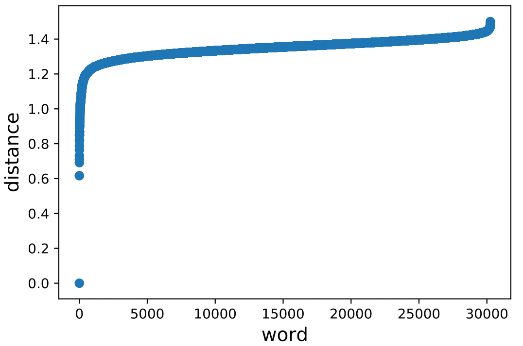
Figure 1: Distances from embeddings of all words in the vocabulary of Amazon dataset to the word “cat”.

For checking whether this behaviour persists for other words, we computed all the distances between embeddings from the words of the Reuters dataset. Figure 2 shows the distribution of these distances clustered in bins for better visualization. Once again, we observe a high concentration of the distances around the interval $[1.2,1.4]$, behaving similarly to a Normal distribution.

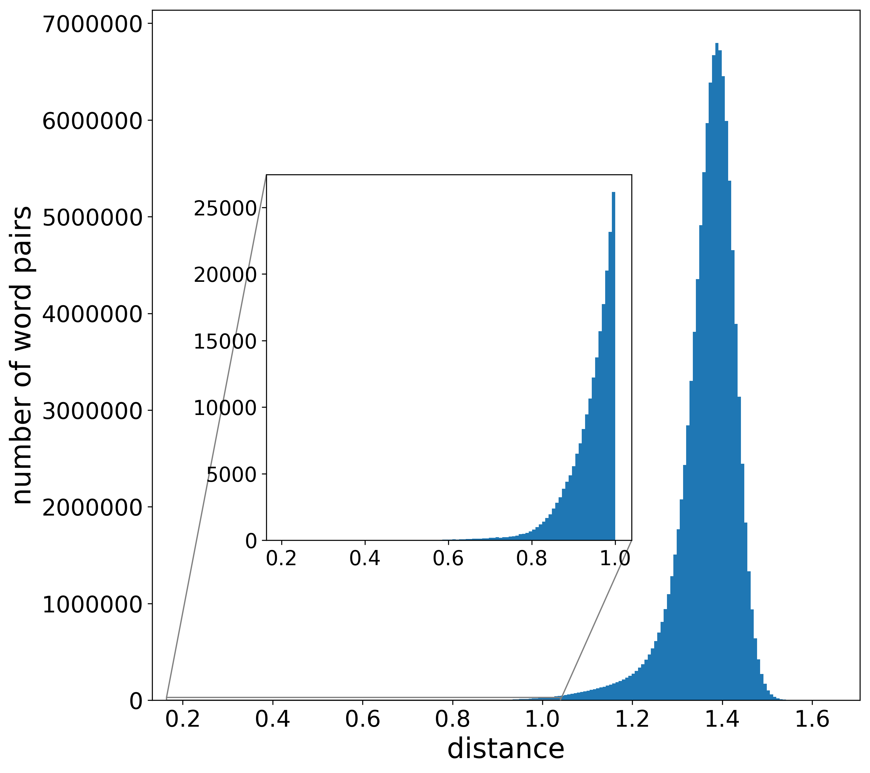
Figure 2: Distribution of the distances between all words in the vocabulary of Reuters dataset.

Based on this discussion, we make the following assumptions:

1. Given a word $w$, the remaining words can be split into two groups: RELATED($w$) and UNRELATED($w$), with the former (latter) containing the words related (unrelated) with $w$;

2. The distances from every word in UNRELATED($w$) to $w$, for every $w$, is the same “large” value $c_{max}$.

Although the number of related words may vary according to the word of reference, in order to make our approach simpler and thus, more practical, we assume that all words have the same number of related words and we use $r$ to denote this number. The value of $r$ can either be set manually or automatically estimated using a training set as we discuss in the experimental section.

3.2 Algorithms exploiting distance assumptions

Algorithms to compute distances with the flavour of WMD can benefit from our assumptions because, by using them, they just need to handle a much smaller set of distances between embeddings, that is, the set of distances between related words. As a result, caching distances becomes feasible even for large vocabularies, which prevent these methods of calculating the distance between the same pair of words more than once. In addition, the transportation problem in which WMD and related distances as RWMD rely on can be solved in a sparse bipartite graph rather than on a complete bipartite graph.

In the next subsections we discuss how WMD and RWMD can be adapted to make use of our assumptions. These adaptations lead to new distances between documents, namely Rel-WMD and Rel-RWMD. We start with the explanation of a preprocessing phase that is required to calculate these new distances.

3.2.1 Preprocessing Phase

In this phase, we build a structure (cache) $C$ that stores for each word $w$, from a vocabulary of $n$ words, the $r$ closest words to $w$ as well as its distances to $w$.

Choose a word $i$ in the vocabulary. The procedure computes its Euclidean distance $\|{\bf x}(i)-{\bf x}(j)\|_{2}$ to every other word $j$ and add these distances, as well as the corresponding words, to a list $L_{i}$. Next, it selects the $r$ words that are closest to $i$ in $L_{i}$ and adds them, with their distances, to cache $C$. This selection can be performed in expected linear time using QuickSelect [11]. The distances that were not included in $C$ are then added to a global accumulator $A$ with the goal of calculating $c_{max}$. This procedure is repeated for every word $i$ in the vocabulary and the value $c_{max}$ is given by the average of all values added to $A$.

The cache $C$ requires $O(n\cdot r)$ space and its construction requires $O(n^{2}\cdot d)$ time, where the term $d$ is due to the time required to compute the distance between a pair of embeddings.

For large vocabularies the construction of the cache $C$, as above described, may be costly due to the $O(n^{2}\cdot d)$ time complexity. This construction, however, can be optimized by clustering the embeddings and then considering only words in the same cluster to find the related words.

We discuss this approach using the traditional $k$-means clustering algorithm [1]. On the one hand, this algorithm allows the user to define the number of clusters $k$ and it performs $O(n\cdot k\cdot d\cdot I)$ operations to cluster $n$ points in $R^{d}$ into $k$ clusters, where $I$ is the maximum number of iterations allowed. On the other hand, if the $n$ embeddings are uniformly distributed among $k$ clusters then the construction of cache $C$ requires $O((n/k)^{2}\cdot d)$ time per cluster which implies on $O(n^{2}\cdot d/k)$ overall time. Hence, let $f(k)=n\cdot d\cdot k\cdot I+(n^{2}\cdot d/k)$ be an estimation of the running time required to execute $k$-means and then the construction of cache $C$. By minimizing $f(k)$ we get $k=\sqrt{n/I}$. Thus, if $n$ is large, in order to speed up the preprocessing phase, we run $k$-means algorithm with $k=\sqrt{n/I}$, before building the cache $C$.

3.2.2 Related Word Mover’s Distance

The Related Word Mover’s Distance (Rel-WMD) between $D$ and $D^{\prime}$ is defined as the optimum value of the transportation problem given by equations (1)-(4), where the costs of the edges are as follows:

$$c(w_{i},w^{\prime}_{j})=\begin{cases}0,&\mbox{ if }w_{i}=w^{\prime}_{j}\\ \|{\bf x}(w_{i})-{\bf x}(w^{\prime}_{j})\|_{2},&\mbox{ if }(w_{i},w^{\prime}_{j})\in C\\ c_{max},&\mbox{otherwise}\end{cases}$$ (6)

For small values of parameter $r$ many costs are equal to $c_{max}$. In this case, it is possible to replace the formulation given by (1)-(4) with an equivalent and more compact one. This new formulation is given by (7)-(10) and its key idea is using variable $T_{i,t}$ to represent the number of units of word $w_{i}$ that is transformed into words that are at a distance $c_{max}$ from $w_{i}$. Thus, the single variable $T_{i,t}$ replaces all variable $T_{i,j}$ in the original formulation for which $(w_{i},w^{\prime}_{j})$ does not belong to cache $C$. Similarly $T_{t,j}$ represents the number of units transformed into $w^{\prime}_{j}$ from words that are at a distance $c_{max}$ of word $w^{\prime}_{j}$. The underlying graph of this new formulation is much sparser (for small values of $r$) so that the transportation problem can be solved significantly faster.

min $$\displaystyle\sum\limits_{(w_{i},w^{\prime}_{j})\in C}c(w_{i},w^{\prime}_{j})T_{i,j}+\displaystyle\sum\limits_{i=1}^{|D|}c_{max}T_{i,t}$$ (7)

s.t.: $$\,\,T_{i,t}+\displaystyle\sum\limits_{j|(w_{i},w^{\prime}_{j})\in C}T_{i,j}=D_{i} i=1,\dots,|D|$$ (8)

$$T_{t,j}+\displaystyle\sum\limits_{i|(w_{i},w^{\prime}_{j})\in C}T_{i,j}=D^{\prime}_{j} j=1,\dots,|D^{\prime}|$$ (9)

$$T_{i,j},T_{i,t},T_{t,j}\geq 0 \text{for all }\quad i,j$$ (10)

We shall note that this formulation has been used before by [19] to speed up EMD [23] in the context of image retrieval.

3.2.3 Related Relaxed Word Mover’s Distance

The Related Relaxed Word Mover ’s Distance (Rel-RWMD) is a variation of the Rel-WMD, in which we drop constraints of the original formulation in order to obtain a relaxation that can be computed more efficiently. Rel-RWMD is to Rel-WMD as RWMD is to WMD.

The Rel-RWMD can be computed using equation (5) with a cost structure given by (6). Let $R^{\prime}(w_{i})$ (resp. $R(w^{\prime}_{j})$ ) be the set of related words of $w_{i}$ (resp. $w^{\prime}_{j}$) that belong to $D^{\prime}$ (resp. $D$). Thus, the Rel-RWMD between documents $D$ and $D^{\prime}$ is given by

$$\max\left\{\sum_{i=1}^{|D|}D_{i}\min_{w^{\prime}_{j}\in R^{\prime}(w_{i})}c(w_{i},w^{\prime}_{j}),\sum_{j=1}^{|D^{\prime}|}D^{\prime}_{j}\min_{w_{i}\in R(w^{\prime}_{j})}c(w_{i},w^{\prime}_{j})\right\}$$ (11)

Although not explicit in the above equation, if $R^{\prime}(w_{i})$ (resp. $R(w^{\prime}_{j}))$ is empty then $D_{i}$ (resp. $D^{\prime}_{j}$) is multiplied by $c_{max}$.

To efficiently evaluate the first term of the maximum in equation (11) we need to obtain for each $w$ in $D$ its related words that belong to $D^{\prime}$, that is, the set $R^{\prime}(w)$. By storing $D^{\prime}$ as a hash table we can find them in $O(r)$ time. For that, it is enough to traverse the list of words related to $w$ in cache C and for each word $w^{\prime}$ in the list we use the hash table of $D^{\prime}$ to verify whether $w^{\prime}$ belongs to $D^{\prime}$. Since the second term in the maximum can be calculated analogously we conclude that the Rel-RWMD between $D$ and $D^{\prime}$ can be computed in $O((|D|+|D^{\prime}|)\cdot r)$ time, which is a significant improvement over the $(|D|\cdot|D^{\prime}|)$ time required by RWMD when the size of the documents is considerably larger than $r$.

Finally, we mention that the linear time implementation of RWMD presented in Section 2.3.1 can also benefit from our assumptions. The first advantage is that the matrix $M$ can be computed faster since, in order to fill the row associated with a document $D$, we just need to consider the words in the vocabulary that are related to $D$ because for the other words the corresponding entries have value $c_{max}$. Thus, the addition of the row associated with document $D$ costs $O(|D|\cdot r)$ time rather than the $O(n\cdot|D|\cdot d)$ required by RWMD(L). The second advantage is the sparsity of matrix $M$ which allows handling larger collections/vocabularies.

4 EXPERIMENTS

To evaluate our methods, we employ two tasks that involve the computation of distances between documents. The first one is the document classification task via $k$-Nearest Neighbors ($k$-NN) that was used to evaluate the WMD algorithm in [14]. The second one is the task of identifying related pairs of documents, employed to evaluate the performance of paragraph vector [15, 6].

We compared in terms of test error and computational performance our new distance, Rel-RWMD, against WMD, RWMD, Cosine distance and Word Centroid Distance (WCD) [14]. The WCD between two documents is given by the Euclidean distance between their centroids, where the centroid of a document $D$ is defined as $\sum_{i=1}^{|D|}D_{i}x(w_{i})$. When reporting computational times we use RWMD(S) and RWMD(L) to distinguish between the Standard implementation of RWMD and the one that requires Linear time. Rel-RWMD(S) and Rel-RWMD(L) are used analogously. We note that for all RWMD’s implementations the preprocessing described at the end of Section 2.3 is applied.

Although we have also implemented/evaluated Rel-WMD, its results are omitted in the next sections since, in general, it is competitive with Rel-RWMD in terms of test error while being much slower.

The methods were implemented in C++. The Eigen library [10] was used for matrix manipulation and Linear Algebra while the OR-Tools library [21] was used for the resolution of flow problems. All experiments were executed using a single core of an Intel(R) Core(TM) i7-6700 CPU @ 3.40GHz, with 8 GB of RAM. The code and datasets are available in a GitHub repository .

4.1 Document classification via $k$-NN

Our experimental setting follows Kusner et al. [14], where different distances are evaluated according to their performance when they are employed by the $k$-NN method to address document classification tasks.

In order to classify a document $D$ from some testing set, $k$-NN computes the distance of $D$ to each document in the corresponding training set and then it returns the most frequent class among the $k$ closest documents to $D$. As stated in [14], motivations for using this evaluation approach, based on $k$-NN , include its reproducibility and simplicity.

We run $k$-NN using $k=19$, and, in case of ties, $k$ is divided by two until there are no more ties. This setting is slightly different from [14], where $k$ is selected from the set $\{1,3,\ldots,19\}$ based on the lower error rate obtained.

The parameter $r$ that defines the number of related words was selected from the set $S=\{1,2,4,\dots,128\}$ using a $5$-fold cross-validation on top of the training set. Because we are prioritizing computational performance and, the smaller the $r$ the faster the method, we choose the lowest $r$ whose test error in the cross validation is at most $1\%$ larger than the minimum one found among all the possibilities in the set $S$.

4.1.1 Datasets description

We used the following eight preprocessed datasets provided by [14]:

• 20NEWS: Posts on discussion boards for 20 different topics.

• AMAZON: Product reviews from Amazon for 4 product categories.

• BBCSPORT: BBC Sport sports section articles for 5 sport between 2004 and 2005.

• CLASSIC: Sentences from academic works from 4 different publishers.

• OHSUMED: Medical summaries categorized by different cardiovascular diseases. For computational performance issues, only the first 10 categories of the database were used.

• RECIPE: Culinary recipes separated by 15 regions of origin.

• REUTERS: News from the Reuters news agency in 1987. The original database contains 90 classes, however, due to problems of imbalance between them, a reduced version with only the 8 most frequent ones was created.

• TWITTER: Collection of tweets labeled by feelings “negative”, “positive” and “neutral”.

For all datasets $70\%$ is used for training and $30\%$ for testing, respecting the partitions provided. Table 1 presents relevant statistics for each of these datasets.

Table 1: Datasets statistics including training and testing sets.

Name	#Docs	$\#$Tokens	Avg. tokens per Doc	Classes
20news	18,820	22,439	69.3	20
amazon	8,000	30,249	44.5	4
bbcsport	737	10,103	116.5	5
classic	7,093	18,080	38.6	4
ohsumed	9,152	19,954	60.2	10
recipe	4,370	5,225	48.3	15
reuters	7,674	15,115	36.0	8
twitter	3,108	4,489	9.9	3

4.1.2 Results

Table 2 presents the test errors obtained by the distances under consideration over the eight datasets. We averaged the results for the datasets AMAZON, BBCSPORT, CLASSIC, RECIPE, and TWITTER following the $5$ predefined train/test splits. The remaining datasets have only one split, and so the average is not necessary.

Some observations are in order: clearly, WCD and Cosine presented the worst results. Among WMD, RWMD, and Rel-RWMD, there is a balance. The behaviour of WCD and Cosine, as well as the balance between WMD and RWMD, are compatible with the findings/conclusions reached in [14] while the results of Rel-RWMD suggest that our simplifying assumptions work very well. The values selected for $r$ ranged from 2 (20NEWS and RECIPE) to 128 (AMAZON) with a median equal 19.5.

Table 2: Test error (in %) for different distances and datasets. The datasets with more than one partition had their error rates averaged. The best results are bold faced.

Dataset	Cosine	WCD	WMD	RWMD	Rel-RWMD
20news	30.45	36.2	24.09	24.79	25.22
amazon	12.90	9.04	7.21	6.87	6.98
bbcsport	4.82	11.9	5.36	5.09	4.82
classic	6.34	8.93	3.04	2.91	3.15
ohsumed	45.74	47.00	42.85	43.49	41.26
recipe	45.71	49.20	46.56	43.63	43.20
reuters	8.95	4.98	3.84	3.97	4.39
twitter	31.97	29.4	29.14	28.95	28.95
average	23.36	24.59	20.26	19.94	19.75

Table 3 presents the running times in minutes for all distances and datasets examined. First, as expected, WCD and Cosine are the fastest distances since they run in linear time and their preprocessing phases are very cheap while WMD is the slowest distance since it has to solve a transportation problem optimally. We note that the times of Cosine were omitted due to the lack of space.

It is interesting to examine how the distances/implementations related to RWMD perform. RWMD(S), the original implementation of [14], is the slowest of them while Rel-RWMD(L) is the fastest one, being on average 4.7 times faster than RWMD(L), which is the second fastest. The main advantage of Rel-RWMD(L) over RWMD(L) is due to the time required to build the matrix $M$ since Rel-RWMD(L) is, on average, 10 times faster. With regards to the time required to evaluate two doc’s we can also observe a small advantage of Rel-RWMD(L) which is probably related to the sparsity of $M$.

Table 3: Computational runtime (in minutes) for different distances and datasets. The datasets with more than one partition have their computational times averaged.

Dataset	WCD	WMD	RWMD(S)	RWMD(L)	Rel-RWMD(L)
20news	1.87	6,244	842	68.0	13.4
amazon	0.30	351	71.7	22.1	4.47
bbcsport	0.01	21	3.72	1.38	0.27
classic	0.24	213	45.6	10.8	2.26
ohsumed	0.47	1,002	158	25.1	5.20
recipe	0.09	106	27.6	2.13	0.55
reuters	0.27	181	47.7	10.9	1.67
twitter	0.04	3.32	1.23	0.43	0.18

It is important to mention that the values in Table 3 do not include the time required to estimate the value of $r$. In fact, the execution of a 5-fold cross validation on the training set for each potential $r$ incurs a high cost. However, in practice one can estimate the value of $r$ using a much smaller set or, even better, set $r$ to a small value, without estimating it, as suggested by the results of Table 4. This table presents the test errors for $r=1,2,16,128$ and also for the value estimated via cross validation. We observe that the test errors remain at the same level, in particular for $r\geq 16$. The running times, though not presented, change very little as expected since the value of $r$ has a small effect in the time complexity of the linear implementation of Rel-RWMD.

Table 4: Test Error (in %) for Rel-RWMD, with $r=1,2,\ 16,\ 128$ and values estimated via cross-validation, for the different datasets.

dataset	Cross Val.	r=1	r=2	r=16	r=128
20news	25.22	25.27	25.22	24.90	25.22
amazon	6.98	9.66	9.21	7.94	7.02
bbcsport	4.82	4.00	3.64	4.91	5.55
classic	3.15	3.62	3.56	3.20	3.18
ohsumed	41.26	42.44	42.83	41.26	41.55
recipe	43.20	43.57	43.20	43.20	43.52
reuters	4.39	4.93	4.52	4.02	4.20
twitter	28.95	31.52	30.60	28.91	29.16
Average	19.75	20.63	20.35	19.79	19.92

4.2 Identifying related documents

For the second task our experimental setting is inspired on Dai et al. [6], where representations/distances are evaluated according to their capacity of recognizing whether a document $D^{1}$ is more related to a document $D^{2}$ or to a document $D^{3}$. For achieving this goal, testing sets are used which contain many triples of documents, namely triplets. In each triplet, only two documents are related and a given distance succeeds if its smallest value is achieved for the related pair.

4.2.1 Datasets description

For our experiments, we first downloaded the documents in the two testing sets of triplets provided in [6]. The first set uses papers from Arxiv while the second one uses articles from Wikipedia. Then, we preprocessed them to remove all non-alphanumeric characters and words contained in a list of stopwords due to its little semantic value. Finally, to represent the documents we just consider the words that have embeddings in the set that Google made available. It is important to note that we are not using the embeddings of [6] since they were not provided. Table 5 presents relevant statistics for each of the datasets.

Table 5: Datasets statistics.

Name	#Docs	#Triplets	$\#$Tokens	Avg. tokens per Doc
Arxiv	47,080	19,998	260,640	1,043.9
Wikipedia	58,015	19,336	415,967	429.8

4.2.2 Results

In this experiment, in contrast to the previous one, each document has its distance evaluated a few times on average, indeed less than twice. Thus, building the cache $M$ required for the linear time implementations of RWMD does not pay off. In addition, its size would be huge, around $10^{10}$ entries for Wikipedia as an example. Therefore, we only executed RWMD(S) and Rel-RWMD(S).

By comparing the statistics of the datasets in Tables 1 and 5, we observe that the number of tokens (word embeddings) of the latter is one order of magnitude higher than the former and, as a consequence, the preprocessing phase of Rel-RWMD becomes expensive, harming the performance gain achieved while computing the distances. Thus, following our approach, we cluster the embeddings before building the cache $C$. We run $k$-means using a limit of $I=5$ iterations and setting $k=289\approx\sqrt{415,967/5}$ for Wikipedia and $k=229\approx\sqrt{260,640/5}$ for Arxiv. Moreover, motivated by the discussion/results of the previous section we used $r=16$ for Rel-RWMD.

Table 6 presents the test errors achieved by the different methods. We can observe a behaviour similar to the previous task. Once again, both Cosine and WCD achieve the largest test errors while the others display competitive results.

Table 6: Test Error (in %) for different distances and datasets. The best results are bold faced.

Dataset	Cosine	WCD	WMD	RWMD	Rel-RWMD
Arxiv	28.83	29.99	22.77	23.43	23.16
Wikipedia	27.83	29.23	26.74	27.01	26.90

The computational times (in minutes) are displayed in Table 7. Again WCD and Cosine are the fastest. The former is slower because it has to compute the centroids of the documents in its preprocessing phase while the latter does not. Among the others, Rel-RWMD(S) and RWMD(S), as expected, are much faster than WMD. For Wikipedia Rel-RWMD(S) is 3 times faster than RWMD(S) while for Arxiv Rel-RWMD(S) it is 27 times faster.

By taking a more in-depth examination of the running times we can also observe that the time consumption of REL-RWMD(S) is highly concentrated on its preprocessing phase when the cache $C$ is built. Having this structure available, it computes the distances, on average, 25 and 60 times faster than RWMD(S) for Wikipedia and Arxiv, respectively.

Table 7: Computational runtime (in minutes) for different distances and datasets.

Dataset	Cosine	WCD	WMD	RWMD(S)	Rel-RWMD(S)
Arxiv	0.01	0.18	1,996	74.8	2.72
Wikipedia	0.01	0.09	302	11.0	3.36

5 CONCLUSION

In this paper, we presented an approach to speed up the computation of WMD and its variants that relies on the properties of the distances between embeddings. The improvements in time and space complexities together with our experimental evaluation provide strong evidence that this approach should be employed if one is aiming to compute these distances efficiently.

The second author is partially supported by CNPq under grant 307572/2017-0 and by FAPERJ, grant Cientista do Nosso Estado E-26/202.823/2018.

References

- [1] David Arthur and Sergei Vassilvitskii, ‘k-means++: The advantages of careful seeding’, in Proceedings of the eighteenth annual ACM-SIAM symposium on Discrete algorithms, pp. 1027–1035. Society for Industrial and Applied Mathematics, (2007).
- [2] Kubilay Atasu and Thomas Mittelholzer, ‘Linear-complexity data-parallel earth mover’s distance approximations’, in International Conference on Machine Learning, pp. 364–373, (2019).
- [3] Kubilay Atasu, Thomas Parnell, Celestine Dünner, Manolis Sifalakis, Haralampos Pozidis, Vasileios Vasileiadis, Michail Vlachos, Cesar Berrospi, and Abdel Labbi, ‘Linear-complexity relaxed word mover’s distance with gpu acceleration’, in 2017 IEEE International Conference on Big Data (Big Data), pp. 889–896. IEEE, (2017).
- [4] David M Blei, Andrew Y Ng, and Michael I Jordan, ‘Latent dirichlet allocation’, Journal of machine Learning research, 3(Jan), 993–1022, (2003).
- [5] Marco Cuturi, ‘Sinkhorn distances: Lightspeed computation of optimal transport’, in Advances in neural information processing systems, pp. 2292–2300, (2013).
- [6] Andrew M Dai, Christopher Olah, and Quoc V Le, ‘Document embedding with paragraph vectors’, arXiv preprint arXiv:1507.07998, (2015).
- [7] Rajarshi Das, Manzil Zaheer, and Chris Dyer, ‘Gaussian lda for topic models with word embeddings’, in Proceedings of the 53rd Annual Meeting of the Association for Computational Linguistics and the 7th International Joint Conference on Natural Language Processing (Volume 1: Long Papers), volume 1, pp. 795–804, (2015).
- [8] Susan T Dumais, George W Furnas, Thomas K Landauer, Scott Deerwester, and Richard Harshman, ‘Using latent semantic analysis to improve access to textual information’, in Proceedings of the SIGCHI conference on Human factors in computing systems, pp. 281–285. Acm, (1988).
- [9] Aude Genevay, Marco Cuturi, Gabriel Peyré, and Francis Bach, ‘Stochastic optimization for large-scale optimal transport’, in Advances in Neural Information Processing Systems, pp. 3440–3448, (2016).
- [10] Gaël Guennebaud, Benoît Jacob, et al. Eigen v3. http://eigen.tuxfamily.org, 2010.
- [11] Charles AR Hoare, ‘Algorithm 65: find’, Communications of the ACM, 4(7), 321–322, (1961).
- [12] Andreas Hotho, Steffen Staab, and Gerd Stumme, ‘Ontologies improve text document clustering’, in Data Mining, 2003. ICDM 2003. Third IEEE International Conference on, pp. 541–544. IEEE, (2003).
- [13] Gao Huang, Chuan Guo, Matt J Kusner, Yu Sun, Fei Sha, and Kilian Q Weinberger, ‘Supervised word mover’s distance’, in Advances in Neural Information Processing Systems, pp. 4862–4870, (2016).
- [14] Matt Kusner, Yu Sun, Nicholas Kolkin, and Kilian Weinberger, ‘From word embeddings to document distances’, in International Conference on Machine Learning, pp. 957–966, (2015).
- [15] Quoc Le and Tomas Mikolov, ‘Distributed representations of sentences and documents’, in International Conference on Machine Learning, pp. 1188–1196, (2014).
- [16] Chenliang Li, Haoran Wang, Zhiqian Zhang, Aixin Sun, and Zongyang Ma, ‘Topic modeling for short texts with auxiliary word embeddings’, in Proceedings of the 39th International ACM SIGIR conference on Research and Development in Information Retrieval, pp. 165–174. ACM, (2016).
- [17] Tomas Mikolov, Kai Chen, Greg Corrado, and Jeffrey Dean, ‘Efficient estimation of word representations in vector space’, arXiv preprint arXiv:1301.3781, (2013).
- [18] Tomas Mikolov, Ilya Sutskever, Kai Chen, Greg S Corrado, and Jeff Dean, ‘Distributed representations of words and phrases and their compositionality’, in Advances in neural information processing systems, pp. 3111–3119, (2013).
- [19] Ofir Pele and Michael Werman, ‘Fast and robust earth mover’s distances’, in Computer vision, 2009 IEEE 12th international conference on, pp. 460–467. IEEE, (2009).
- [20] Jeffrey Pennington, Richard Socher, and Christopher Manning, ‘Glove: Global vectors for word representation’, in Proceedings of the 2014 conference on empirical methods in natural language processing (EMNLP), pp. 1532–1543, (2014).
- [21] Laurent Perron and Vincent Furnon. Or-tools. https://developers.google.com/optimization/.
- [22] Gabriel Peyré and Marco Cuturi, ‘Computational optimal transport’, Foundations and Trends® in Machine Learning, 11(5-6), 355–607, (2019).
- [23] Yossi Rubner, Carlo Tomasi, and Leonidas J Guibas, ‘A metric for distributions with applications to image databases’, in Computer Vision, 1998. Sixth International Conference on, pp. 59–66. IEEE, (1998).
- [24] Claude Elwood Shannon, ‘A mathematical theory of communication’, Bell System Technical Journal, 27(July & October), 379–423 & 623–656, (1948).
- [25] Lingfei Wu, Ian EH Yen, Kun Xu, Fangli Xu, Avinash Balakrishnan, Pin-Yu Chen, Pradeep Ravikumar, and Michael J Witbrock, ‘Word mover’s embedding: From word2vec to document embedding’, (2018).