Fast Stochastic Ordinal Embedding with Variance Reduction and Adaptive Step Size

Abstract

Learning representation from relative similarity comparisons, often called ordinal embedding, gains rising attention in recent years. Most of the existing methods are based on semi-definite programming (SDP), which is generally time-consuming and degrades the scalability, especially confronting large-scale data. To overcome this challenge, we propose a stochastic algorithm called SVRG-SBB, which has the following features: i) achieving good scalability via dropping positive semi-definite (PSD) constraints as serving a fast algorithm, i.e., stochastic variance reduced gradient (SVRG) method, and ii) adaptive learning via introducing a new, adaptive step size called the stabilized Barzilai-Borwein (SBB) step size. Theoretically, under some natural assumptions, we show the $\boldsymbol{O}(\frac{1}{T})$ rate of convergence to a stationary point of the proposed algorithm, where $T$ is the number of total iterations. Under the further Polyak-Łojasiewicz assumption, we can show the global linear convergence (i.e., exponentially fast converging to a global optimum) of the proposed algorithm. Numerous simulations and real-world data experiments are conducted to show the effectiveness of the proposed algorithm by comparing with the state-of-the-art methods, notably, much lower computational cost with good prediction performance.

1 Introduction

Ordinal embedding aims to learn the representation of data as points in a low-dimensional embedded space. Here the “low-dimensional” means the embedding dimension is much smaller than the number of data points. The distances between these points agree with a set of relative similarity comparisons. Relative comparisons are often collected via the participators who are asked to answer questions like:

“Is the similarity between object $i$ and $j$ larger than the similarity between $l$ and $k$?”

The feedback of these questions provide us with a set of quadruplets, i.e., $(i,j,l,k)$ which indicates that the similarity between object $i$ and $j$ is larger than the similarity between $l$ and $k$. These relative similarity comparisons are the supervision information for ordinal embedding. Without prior knowledge, the relative similarity comparisons always involve all objects, and the number of potential quadruplets could be $\boldsymbol{O}(n^{4})$. Even under the so-called “local” setting where we restrict $l=i$, the triple-wise comparisons, $(i,j,k)$, also have the complexity $\boldsymbol{O}(n^{3})$.

The ordinal embedding problem was firstly studied by [1, 2, 3, 4] in the psychometric society. In recent years, it has drawn a lot of attention in machine learning [5, 6, 7, 8, 9, 10], statistic ranking [11, 12, 13], artificial intelligence [14, 15], information retrieval [16], and computer vision [17, 18], etc.

Most of the ordinal embedding methods are based on the semi-definite programming (SDP). Some typical methods include the Generalized Non-Metric Multidimensional Scaling (GNMDS) [19], Crowd Kernel Learning (CKL) [20], and Stochastic Triplet Embedding (STE/TSTE) [21]. The main idea of such methods is to formulate the ordinal embedding problem into a convex, low-rank SDP problem with respect to the Gram matrix of the embedding points. In order to solve such a SDP problem, the traditional methods generally employ the projection gradient descent to satisfy the positive semi-definite constraint, where the singular value decomposition (SVD) is required at each iteration. This inhibits the popularity of this type of methods for large-scale and online ordinal embedding applications.

To handle the large-scale ordinal embedding problem, we reformulate the considered problem using the embedding matrix instead of its Gram matrix. By taking advantage of this new non-convex formulation, the positive semi-definite constraint is eliminated. Furthermore, we exploit the well-known stochastic variance reduced gradient (SVRG) method to efficiently solve the developed formulation, which is a fast stochastic algorithm proposed in [22]. Generally, step size, one essential hyper-parameter, should be tuned in SVRG. It is a difficult task in practice as the Lipschitz constant is hard to estimate. To facilitate the use of SVRG, Tan et al. [23] introduced the well-known, adaptive step size called the Barzilai-Borwein (BB) step size [24], and proved its linear convergence in the strongly convex case. However, as shown in our simulations (see, Figure 1), the absolute value of the original BB step size varies dramatically regarding the epoch number, when applied to our developed ordinal embedding formulation. One major reason is that our developed ordinal embedding model is not strongly convex, and even non-convex. Thus, in such setting, the denominator of BB step size might be very close to zero, leading to the instability of the BB step size. We add another positive term to the non-negative denominator of BB step size which overcomes such instability of the original BB step size. Similar to the original version, the new step size is adaptive with almost the same computational cost. More importantly, the new step size is more stable than the original BB step size, and can be applied to more general case beyond the strongly convexity assumption. Henceforth, we call the new method as stabilized Barzilai-Borwein (SBB) step size. By incorporating the SBB step size with SVRG, we propose a new stochastic algorithm called SVRG-SBB for efficiently solving the considered ordinal embedding model.

In summary, our main contributions can be shown as follows:

• We propose a non-convex framework for the ordinal embedding problem via considering the original embedding variable rather than its Gram matrix. We get rid of the positive semi-definite (PSD) constraint on the Gram matrix, and thus, our proposed algorithm is SVD-free and has better scalability than the existing convex ordinal embedding methods.

• The introduced SBB step size can overcome the instability of the original BB which comes from the absence of strongly convexity. More importantly, the proposed SVRG-SBB algorithm outperforms most of the state-of-the-art methods as shown by numerous simulations and real-world data experiments, in the sense that SVRG-SBB often significantly reduces the computational cost.

• We establish $\boldsymbol{O}(\frac{1}{T})$ convergence rate of SVRG-SBB in the sense of converging to a stationary point, where $T$ is the total number of iterations. Such result is comparable with the existing convergence results in the literature.

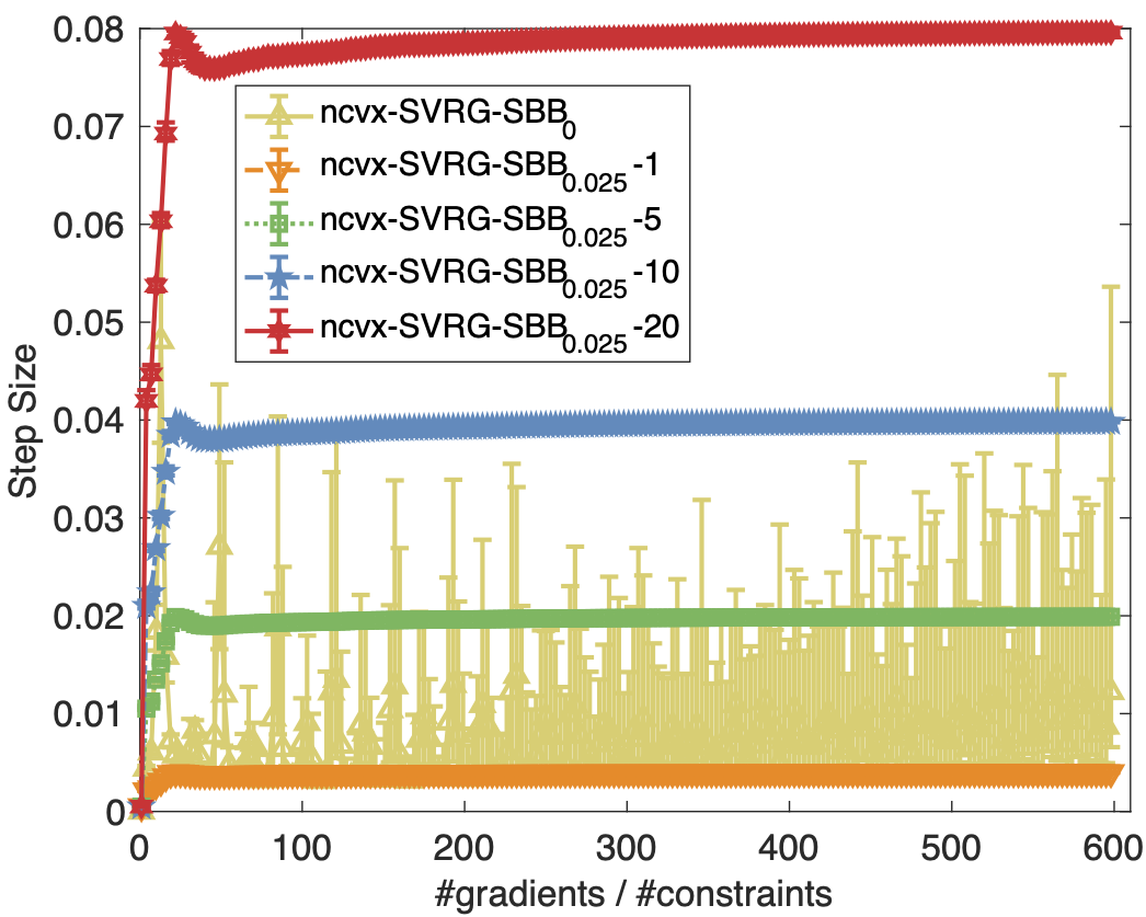
Figure 1: Step sizes along iterations of SVRG-SBB_ϵ on the synthetic data, where the dark yellow curve of ncvx-SVRG-SBB₀ is exactly the varying of the BB step size in this setting.

This paper is an extension of our conference work [25], where we propose the basic SVRG-SBB method which derives the adaptive step size. But there still exist some limitations in our conference method. First, the original SVRG-SBB does not incorporate with mini-batch paradigm which provides a computationally efficient process than single point update. Second, we observe that the well-known “local optimal” of non-convex problem does not have serious impact on the embedding result. The empirical success in non-convex ordinal embedding poses a new problem that under what conditions the non-convex stochastic algorithms may find the global optima effectively. We provide a possible answer of this question with the help of the Polyak-Łojasiewicz (PL) condition. Finally, we summarize the existing ordinal embedding method and propose the generalized ordinal embedding framework which generalizes the existing classification-based methods including GNMDS, CKL and STE/TSTE. We hope the new framework will guide the future research directions.

Organization

The remainder of the paper is organized as follows. In Section 2, we describe the mathematical formulation of the generalized ordinal embedding problem. Section 3 shows the development of the SVRG-SBB algorithm for non-convex ordinal embedding. Section 4 establishes the convergence analysis of the proposed algorithm. Comprehensive experimental validation based on simulated and real-world datasets are demonstrated in Section 5. We conclude this paper in Section 6.

2 Generalized Ordinal Embedding

Throughout the paper, we denote scalars, vectors, matrices and sets as lower case letters ($x$), bold lower case letters ($\boldsymbol{x}$), bold capital letters ($\boldsymbol{X}$) and calligraphy upper case letters ($\mathcal{X}$). $x_{i}$ and $x_{ij}$ denote the $i_{\text{th}}$ element of vector $\boldsymbol{x}$ and $(i,j)$ entry of matrix $\boldsymbol{X}$, respectively. For any $\boldsymbol{x}\in\mathbb{R}^{p}$, $\|\boldsymbol{x}\|_{2}$ denotes its $\ell_{2}$ norm. $\boldsymbol{I}_{n}$ is the identity matrix with size $n\times n$ and the subscript $n$ would be omitted if there is no confusion. For any $\boldsymbol{X}\in\mathbb{R}^{p\times n}$, $\|\boldsymbol{X}\|_{F}$ and $\textit{rank}(\boldsymbol{X})$ denote the Frobenius norm and rank of $\boldsymbol{X}$. $\textit{vec}(\boldsymbol{X})$ is the vectorization operator on $\boldsymbol{X}$ by column. For any square matrix $\boldsymbol{G}\in\mathbb{R}^{n\times n}$, $\textit{tr}(\boldsymbol{G})$ is the trace of $\boldsymbol{G}$. $[n]$ is the set of $\{1,\dots,n\}$. For any $\boldsymbol{X}\in\mathbb{R}^{p\times n}$, $\boldsymbol{G}=\boldsymbol{X}^{\top}\boldsymbol{X}$ is the Gram matrix. For any $(\boldsymbol{x}_{i},\boldsymbol{x}_{j})\in\mathcal{X}\times\mathcal{X}$ where $\mathcal{X}\subset\mathbb{R}^{p}$, $d_{ij}=d(\boldsymbol{x}_{i},\boldsymbol{x}_{j})$ is the distance between $\boldsymbol{x}_{i}$ and $\boldsymbol{x}_{j}$, and $\boldsymbol{D}=\{d^{2}(\boldsymbol{x}_{i},\boldsymbol{x}_{i})\}$ is the squared distance matrix of $\boldsymbol{X}$. Here the distance $d:\mathbb{R}^{p}\times\mathbb{R}^{p}\rightarrow\mathbb{R}_{+}$ depends on the embedded space. In case of the Euclidean space, we adopt the Euclidean distance if not specified. $\mathbb{E}[\cdot]$ represents the expectation.

Let $\mathcal{O}=\{\boldsymbol{o}_{1},\dots,\boldsymbol{o}_{n}\}$ be a collection of objects, $\mathcal{X}\subset\mathbb{R}^{p}$ be a low-dimensional embedded space where $p\ll n$, and $\psi^{*}:\mathcal{O}\times\mathcal{O}\rightarrow\mathbb{R}_{+}$ be a dissimilarity function of $\mathcal{O}$ where $\psi^{*}_{ij}$ is the dissimilarity measure between $o_{i}$ and $o_{j}$. The traditional multi-dimensional scaling (MDS) methods embed $\mathcal{O}$ into $\mathcal{X}$ based on $\Psi^{*}=\{\psi^{*}_{ij},\ i,j\in[n],i\neq j\}$. However, there is always a lack of a dissimilarity function $\psi^{*}$ that can evaluate the objects $\mathcal{O}$ properly for real-world applications, e.g., [15, 18, 26, 27]. As an alternative, ordinal embedding methods incorporate human knowledge into the loop and relax the requirement of $\Psi^{*}$.

By collecting a partially ordered set which assesses dissimilarity on a relative scale by human, ordinal embedding methods establish relative dissimilarity of $\mathcal{X}$ and obtain embedding $\boldsymbol{X}=\{\boldsymbol{x}_{i}:\ \boldsymbol{x}_{i}\in\mathcal{X},\ \boldsymbol{o}_{i}\in\mathcal{O},\ i\in[n]\}$

based on the dissimilarity comparisons. Specifically, given a dissimilarity function $\phi:\mathcal{X}\times\mathcal{X}\rightarrow\mathbb{R}_{+}$ and $\phi_{ij}=\phi(\boldsymbol{x}_{i},\boldsymbol{x}_{j})$ is the dissimilarity between $\boldsymbol{x}_{i}$ and $\boldsymbol{x}_{j}$, we collect a set of quadruplets, that is,

$$\mathcal{Q} = \ \ \left\{q\ |\ q=(i,j,l,k),\ (\phi_{ij},\ \phi_{lk})\in\Phi^{2}\right\},$$ (1)

and define $\Phi^{2}$ as

$$\Phi^{2} = \ \ \left\{(\phi_{ij},\phi_{lk})\ |\ \phi_{ij}<\phi_{lk},\ i,\ j,\ l,\ k\in[n],\right.$$ (2)

$$\ \ \ \ \ \ \ \ \ \ \ \ \ \ \ \ \ \ \ \ \left.i\neq j,\ l\neq k,\ (i,j)\neq(l,k)\right\}.$$

Although the embedding $\boldsymbol{X}$ and $\Phi=\{\phi_{ij}\ |\ i,j\in[n],i\neq j\}$ is unknown, human knowledge can help to determine $\phi_{ij}<\phi_{lk}$ or not and generate $\mathcal{Q}$. The goal of ordinal embedding is to estimate $\boldsymbol{X}$ or $\Phi$ based on $\mathcal{Q}$.

One common class of ordinal embedding methods tries to formulate it as a classification problem (generally, a binary classification problem, say, [19, 20, 21, 28, 9]). Given an ordered quadruplet $q=(i,j,l,k)$ and the associated ordered pair $(\phi_{ij},\phi_{lk})$, the corresponding label $y_{q}$ can be defined as follows

$$y_{q}\left\{\begin{matrix}>0,&\phi_{ij}<\phi_{lk},\\ <0,&\phi_{ij}>\phi_{lk}.\end{matrix}\right.$$ (3)

Here we ignore the multi-class case, e.g. $y_{q}$ could be $\{-1,0,+1\}$ and $y_{q}=0$ indicates that $\phi_{ij}$ and $\phi_{lk}$ have the same value. As it is exceptionally rare in the practical applications and has no obvious improvement of the results whether we include multi-class label or not, we only consider the binary case in our generalized ordinal embedding (GOE) problem.

Let $\mathcal{Y}_{\mathcal{Q}}:=\{y_{q},q\in\mathcal{Q}\}$ be the corresponding label set. Given an embedding candidate $\boldsymbol{X}$ and a classifier $h:\mathbb{R}_{+}\times\mathbb{R}_{+}\rightarrow\mathcal{Y}_{\mathcal{Q}}$, the empirical misclassification error can be defined as follows

$$\mathcal{L}_{\mathcal{Q},\phi,h}(\boldsymbol{X},\mathcal{Y}_{\mathcal{Q}})=\frac{1}{|\mathcal{Q}|}\sum_{q\in\mathcal{Q}}\ell(h(\phi(\boldsymbol{x}_{i},\boldsymbol{x}_{j}),\phi(\boldsymbol{x}_{l},\boldsymbol{x}_{k}),y_{q})),$$ (4)

where $|\mathcal{Q}|$ represents the cardinality of the set $\mathcal{Q}$, and $\ell:\mathbb{R}\times\mathbb{R}\rightarrow\mathbb{R}_{+}\cup\{0\}$ is a specific loss function such as hinge loss or logistic loss. Therefore, the GOE problem can be formulated as the following minimization problem,

$$\underset{\boldsymbol{X}\in\mathbb{R}^{p\times n}}{\min}\ \ \mathcal{L}_{\mathcal{Q},\phi,h}(\boldsymbol{X},\mathcal{Y}_{\mathcal{Q}}).$$ (5)

In practice, the dissimilarity function $\phi$ is generally taken as the squared Euclidean distance $\phi(\boldsymbol{x}_{i},\boldsymbol{x}_{j})=d^{2}_{ij}=\|\boldsymbol{x}_{i}-\boldsymbol{x}_{j}\|_{2}^{2}$, and the empirical loss (4) can be written as

$$\ \ \mathcal{L}_{\mathcal{Q},\phi,h}(\boldsymbol{X},\mathcal{Y}_{\mathcal{Q}})\ =\ \mathcal{L}_{\mathcal{Q},h}(\boldsymbol{D},\mathcal{Y}_{\mathcal{Q}})$$ (6)

$$= \ \ \frac{1}{|\mathcal{Q}|}\sum_{q\in\mathcal{Q}}\ell(h(d^{2}_{ij},d^{2}_{lk},y_{q})),$$

where $\boldsymbol{D}$ is the squared Euclidean distance matrix of $\boldsymbol{X}$.

Besides (5), the following SDP based formulation of the ordinal embedding is commonly used in the literature ([19, 20, 21]). Let $\boldsymbol{G}=\boldsymbol{X^{\top}X}$ be the Gram matrix of $\boldsymbol{X}$. There exists a bijection between the Gram matrix $\boldsymbol{G}\in\mathbb{S}^{n}_{+}$, $\mathbb{S}^{n}_{+}$ is the $n$-dimensional positive semi-definite cone, the set of all symmetric positive semidefinite matrices in $\mathbb{R}^{n\times n}$ and the squared Euclidean distance matrix $\boldsymbol{D}$ as $d^{2}_{ij}\ =\ \|\boldsymbol{x}_{i}-\boldsymbol{x}_{j}\|_{2}^{2}\ =\ g_{ii}-2g_{ij}+g_{jj}$, where $g_{ij}$ is the $(i,j)$ element of $\boldsymbol{G}$.

We change the variable $\boldsymbol{D}$ in empirical loss (6) as $\boldsymbol{G}$

$$\ \ \mathcal{L}_{\mathcal{Q},h}(\boldsymbol{D},\mathcal{Y}_{\mathcal{Q}})\ =\ \mathcal{L}_{\mathcal{Q},h}(\boldsymbol{G},\mathcal{Y}_{\mathcal{Q}})$$ (7)

$$= \ \ \frac{1}{|\mathcal{Q}|}\sum_{q\in\mathcal{Q}}\ell(h(g_{ii}-2g_{ij}+g_{jj},g_{ll}-2g_{lk}+g_{kk},y_{q})).$$

According to (5), (6) and (7), the ordinal embedding problem can be formulated as the following SDP problem with respect to $\boldsymbol{G}$, i.e.,

$${}\underset{\boldsymbol{G}\in\mathbb{S}^{n}_{+},\ \textit{rank}(\boldsymbol{G})\leq p}{\min}\ \ \mathcal{L}_{\mathcal{Q},h}(\boldsymbol{G},\mathcal{Y}_{\mathcal{Q}}),$$ (8)

the positive semi-definite constraint $\boldsymbol{G}\in\mathbb{S}^{n}_{+}$ or $\boldsymbol{G}\succeq 0$ comes from the fact that the Gram matrix $\boldsymbol{G}$ is positive semi-definite matrix; the rank constraint comes from the fact that $\textit{rank}(\boldsymbol{G})\leq\textit{rank}(\boldsymbol{X})\leq\min(n,p)=p$. Note that the formulation (8) is generally convex. However, the computational complexity of such SDP problem is very high, which degrades the scalability of this kind of methods. This motivates us to directly obtain embedding $\boldsymbol{X}$ from (5).

3 Development of SVRG-SBB

Since (5) is an unconstrained optimization problem, SVD and regularization parameter tuning are both avoided. However, without any prior knowledge on $\mathcal{O}$, the sample complexity of $\mathcal{Q}$ is $\boldsymbol{O}(n^{4})$. Because of the expense of full gradients and inverse of Hessian matrix computation in each iteration, the traditional full batch optimization methods, i.e. gradient descent and (quasi-)Newton method, are not suitable for solving such large-scale problem where $n$ would be larger than thousands. Instead of the full-batch methods, we introduce the stochastic algorithm to solve the non-convex problem (5). One open issue in stochastic optimization is how to choose an appropriate step size in practice. Traditional methods include that using a constant step size to track the iterations, adopting a diminishing step size to enforce convergence, or tuning a step size empirically which can be time-consuming. Recently, [23] proposed to use the Barzilai-Borwein (BB) method to automatically compute step sizes in SVRG for strongly convex objective function. Their method is called “SVRG-BB”. In the following part, we will analyze the existing problem of BB method when it is adopted in the non-convex problem. Furthermore, we propose the stabilized Barzilai-Borwein (SBB) step size which alleviates these issues and establish the non-asymptotic convergence analysis of the proposed “SVRG-SBB” algorithm.

3.1 The Existing Problems of Barzilai-Borwein Method

In machine learning and data mining, we often encounter the unconstrained minimization problem (5) as a finite-sum problem. Let $f_{1},\dots,f_{n}$ be a sequence of vector function as $f_{i}:\mathbb{R}^{p}\rightarrow\mathbb{R}$, and our goal is to obtain an approximation solution of the following finite-sum problem

$$\underset{\boldsymbol{x}}{\min}\ f(\boldsymbol{x})=\frac{1}{n}\sum^{n}_{i=1}f_{i}(\boldsymbol{x}),$$ (9)

where $n$ is the training sample size, and each $f_{i}$ is the cost function or loss function corresponding to the $i^{\text{th}}$ training sample. Regardless the convexity of $f$, the choice of step size in stochastic optimization always depends on the Lipschitz constant of $f$, which is usually difficult to estimate in practice. BB step size has been incorporated with SVRG in [23] but it is restricted to the case where their assumptions are each $f_{i}$ is convex, differentiable and $f$ is strongly convex. This assumptions are adopted due to the use of a strongly-convex regularization such as the squared $\ell_{2}$-norm. However, there are many important large-scale non-convex optimization problems, such as neural network.

The original BB method, proposed by Barzilai and Borwein in [24], has been proven to be very effective in solving nonlinear optimization problems via gradient descent. One possible choice of BB step size $\eta_{t}$ is

$$\eta_{t}=\frac{\|\triangle{\boldsymbol{x}}_{t}\|^{2}}{\triangle{\boldsymbol{x}}_{t}^{\top}\triangle{\boldsymbol{y}}_{t}}$$ (10)

where $\triangle{\boldsymbol{x}}_{t}={\boldsymbol{x}}_{t}-{\boldsymbol{x}}_{t-1}$ and $\triangle{\boldsymbol{y}}_{t}=\nabla f({\boldsymbol{x}}_{t})-\nabla f({\boldsymbol{x}}_{t-1})$. Actually BB step size is a possible solution of the so-called “secant equation”.

As the original BB method approximates the inverse of Hessian matrix of $f$ at $\boldsymbol{x}_{t}$ by $\frac{1}{\eta_{t}}\boldsymbol{I}$, there exist some inherent drawbacks toward extending the step size (10) to non-convex optimization problems. If $f$ is differentiable and $\mu$-strongly convex, it holds that

$$\triangle{\boldsymbol{x}}_{t}^{\top}\triangle{\boldsymbol{y}}_{t}\geq\mu\|\triangle{\boldsymbol{x}}_{t}\|^{2}>0$$ (11)

which implies $\eta_{t}$ is always positive. However, if $f$ is differentiable and convex, we have

$$\triangle{\boldsymbol{x}}_{t}^{\top}\triangle{\boldsymbol{y}}_{t}\geq 0$$ (12)

and (10) might approach $\infty$ when the denominator of (10) is extremely small. Furthermore, if the differentiable function $f$ is non-convex, the denominator of (10) might even be negative that makes BB method fail.

Example 1.

given a quadratic optimization problem

$$\underset{{\boldsymbol{x}}\in\mathbb{R}^{p}}{\min}f({\boldsymbol{x}}):=\frac{1}{2}\boldsymbol{x}^{\top}\boldsymbol{A}{\boldsymbol{x}}$$ (13)

where $\boldsymbol{A}$ is a diagonal matrix with $\{\lambda_{i}\}^{p}_{i=1}$ as the diagonal entries, we set $p=3,\lambda_{1}=1,\lambda_{2}=0,\lambda_{3}=-1$. The initial ${\boldsymbol{x}}_{0}=[0,0,1]^{\top}$ and by gradient descent with BB step size, ${\boldsymbol{x}}_{1}={\boldsymbol{x}}_{0}-\eta_{0}\boldsymbol{A}{\boldsymbol{x}}_{0}=[0,0,1+\eta_{0}]$. The corresponding value of (10) is $-1$. If the initial ${\boldsymbol{x}}_{0}=[0,1,0]^{\top}$, the denominator of (10) is $0$.

3.2 SVRG-SBB for Ordinal Embedding

An intuitive way to overcome the flaw of BB step size is to keep the denominator of (10) positive and control the lower bound of $\triangle\boldsymbol{x}_{t}^{\top}\triangle\boldsymbol{y}_{t}$ in each iteration, which leads to our proposed stabilized Barzilai-Borwein (SBB) step size shown as follows

$$\eta_{\epsilon,t}=\frac{\|\triangle{\boldsymbol{x}}_{t}\|^{2}}{|\triangle{\boldsymbol{x}}_{t}^{\top}\triangle{\boldsymbol{y}}_{t}|+\epsilon\|\triangle{\boldsymbol{x}}_{t}\|^{2}}.$$ (14)

Actually, as shown by our latter convergence result, if the Hessian of the objective function $\nabla^{2}f(\boldsymbol{x})$ is nonsingular and the magnitudes of its eigenvalues are lower bounded by some positive constant $\mu$, then we can take $\epsilon=0$. In this case, we call the referred step size SBB₀ henceforth. Even if we have no information about the Hessian of the objective function in practice, the SBB_ϵ step size with an $\epsilon>0$ is just a more conservative version of SBB₀ step size.

From (14), if the gradient $\nabla f_{i}$ is Lipschitz continuous with constant $L>0$ (i.e., $\|\nabla f_{i}({\boldsymbol{x}})-\nabla f_{i}({\boldsymbol{y}})\|\leq L\|{\boldsymbol{x}}-{\boldsymbol{y}}\|,\forall\ {\boldsymbol{x}},{\boldsymbol{y}}\in\mathbb{R}^{p}$), then the SBB_ϵ step size can be bounded as follows

$$\frac{1}{L+\epsilon}\leq\eta_{\epsilon,t}\leq\frac{1}{\epsilon},$$ (15)

where the lower bound is obtained by the $L$-Lipschitz continuity of $\nabla f$, and the upper bound is directly derived by its specific form. Furthermore, if $\nabla^{2}f(\boldsymbol{x})$ is nonsingular and its eigenvalues have a lower bound $\mu>0$, the bound of SBB₀ becomes

$$\frac{1}{L}\leq\eta_{0,t}\leq\frac{1}{\mu}.$$ (16)

The proposed SVRG-SBB algorithm is described in Algorithm 1. As shown in Figure 1, SBB_ϵ step size with a positive $\epsilon$ can make it more stable when SBB₀ step size is unstable and varies dramatically. Moreover, SBB_ϵ step size usually changes significantly only at the initial several epochs, and then quickly gets very stable. This is mainly because there are many iterations in an epoch of SVRG-SBB, and the algorithm might close to a stationary point after only a few epochs. After the initial epochs, the SBB_ϵ step sizes might be very close to the inverse of the objective function curvature as $\epsilon$ is small enough.

The main difference between Algorithm 1 and the former version is that we adopt mini-batch in the inner loop. Mini-batching is a useful strategy for large-scale optimization problem, especially in multi-core and distributed settings as it greatly helps one exploiting parallelism and reducing the communication burden. When the mini-batch size is $1$, Algorithm 1 reduces to our former algorithm. To incorporate mini-batches, we replace single sample gradient update with sampling (with replacement) a subset $\mathcal{I}_{t}\subset[n]$ with its cardinality $|{\cal I}_{t}|=b$, where $b\in\mathbb{N}$ is the mini-batch size. We update the $\boldsymbol{x}^{s}_{t}$ by the modified SBB step size as ${\boldsymbol{x}}^{s}_{t+1}={\boldsymbol{x}}^{s}_{t}-b\eta_{\epsilon,s-1}{\boldsymbol{u}}^{s}_{t}$, where $\eta_{t,s-1}$ is specified in (17) and $\boldsymbol{u}^{s}_{t}$ is defines as

$${\boldsymbol{u}}^{s}_{t}=\frac{1}{b}\underset{i_{t}\in\mathcal{I}_{t}}{\sum}\left(\nabla f_{i_{t}}({\boldsymbol{x}}^{s}_{t})-\nabla f_{i_{t}}(\tilde{{\boldsymbol{x}}}^{s})\right)+\nabla f(\tilde{\boldsymbol{x}}^{s}).$$

Algorithm 1 SVRG-SBB for (9)

0:  $\epsilon\geq 0$, update frequency $m$, mini-batch size $b$, maximal number of iterations $S$, initial step size $\eta_{0}$ (only used in the first epoch), initial point $\tilde{{\boldsymbol{x}}}^{0}\in\mathbb{R}^{p}$, and the number of training samples $n$

  for $s=0$ to $S-1$ do

     

$$\boldsymbol{g}^{s+1}=\nabla f(\tilde{{\boldsymbol{x}}}^{s})=\frac{1}{n}\sum^{n}_{i=1}\nabla f_{i}(\tilde{{\boldsymbol{x}}}^{s})$$

     if $s>0$ then

        

$$\triangle{\boldsymbol{x}}_{s}=\tilde{{\boldsymbol{x}}}^{s}-\tilde{{\boldsymbol{x}}}^{s-1},\ \triangle{\boldsymbol{x}}_{s}=\ \ \ {\boldsymbol{g}}^{s+1}-{\boldsymbol{g}}^{s},$$

$$\eta_{\epsilon,s}=\frac{1}{m}\cdot\frac{\|\triangle{\boldsymbol{x}}_{s}\|^{2}}{|\langle\triangle{\boldsymbol{x}}_{s},\triangle\boldsymbol{y}_{s}\rangle|+\epsilon\|\triangle{\boldsymbol{x}}_{s}\|^{2}}$$ (17)

     end if

     ${\boldsymbol{x}}^{s+1}_{0}=\tilde{{\boldsymbol{x}}}^{s}$

     for $t=0$ to $m-1$ do

        uniformly pick $\mathcal{I}_{t}\subset[n]$ with $|\mathcal{I}_{t}|=b$

        ${\boldsymbol{u}}^{s+1}_{t}=\frac{1}{b}\underset{i_{t}\in\mathcal{I}_{t}}{\sum}\left(\nabla f_{i_{t}}({\boldsymbol{x}}^{s+1}_{t})-\nabla f_{i_{t}}(\tilde{\boldsymbol{x}}^{s})\right)+\boldsymbol{g}^{s+1}$

        ${\boldsymbol{x}}^{s+1}_{t+1}={\boldsymbol{x}}^{s+1}_{t}-b\eta_{\epsilon,s}{\boldsymbol{x}}^{s+1}_{t}$

     end for

     $\tilde{\boldsymbol{x}}^{s+1}={\boldsymbol{x}}^{s+1}_{m}$

  end for

  ${\boldsymbol{x}_{\mathrm{out}}}$ is chosen uniformly from $\{\{\boldsymbol{x}^{s}_{t}\}_{t=1}^{m}\}_{s=1}^{S}$.

4 Convergence Analysis of SVRG-SBB

In this section, we first establish a sublinear rate of convergence (to a stationary point) of the proposed SVRG-SBB under the mild smoothness condition, and then show the linear rate of convergence (i.e., converging exponentially fast to a global optimum) of its modular version under the furthered Polyak-Łojasiewicz (PL) property [29].

4.1 Sublinear convergence under smoothness

Throughout this section, we assume that each $f_{i}$ in (9) is $L$-smoothness with a constant $L>0$, i.e., $f_{i}$ is continuously differentiable and its gradient $\nabla f_{i}$ is $L$-Lipschitz, shown as follows:

$$\|\nabla f_{i}(\boldsymbol{x})-\nabla f_{i}(\boldsymbol{y})\|\leq L\|\boldsymbol{x}-\boldsymbol{y}\|,\ \forall\ \boldsymbol{x},\boldsymbol{y}\in\mathbb{R}^{p}.$$ (18)

The $L$-smoothness assumption is very general to derive the convergence of an algorithm in literature (say, [30], [31], [32], [33]). As shown in the supplementary material, all the loss functions adopted in the experiments for GOE problem are verified to satisfy this assumption.

In the following, we provide a key lemma that illustrates the convergence behavior of the inner loop of Algorithm 1. To state this lemma, we first define several positive constants and sequences which are used in our analysis. Given a positive sequence $\{\beta_{s}\}_{s=0}^{S-1}$, for any $0\leq s\leq S-1$, we define

$$\rho_{s}:=1+b\eta_{\epsilon,s}\beta_{s}+2b\eta_{\epsilon,s}^{2}L^{2},$$ (19)

and for any $t=0,\ldots,m-1$,

$$c_{t,s}:=\rho_{s}c_{t+1,s}+b\eta_{\epsilon,s}^{2}L^{3}$$ (20)

with ${c}_{m,s}=0$, and

$$\Gamma_{t,s}:=b\eta_{\epsilon,s}\left[1-c_{t+1,s}\beta_{s}^{-1}-b\eta_{\epsilon,s}(L+2c_{t+1,s})\right].$$ (21)

Based on these sequences, we present the lemma as follows.

Lemma 1.

Suppose that each $f_{i}$ is $L$-smoothness (i.e., satisfying (18)). Let $\{{\boldsymbol{x}}_{t}^{s+1}\}_{t=1}^{m}$ be a sequence generated by Algorithm 1 at the $s^{\text{th}}$ inner loop, $s=0,\ldots,S-1$. Let $b,m,\epsilon$ and $\beta_{s}$ be chosen such that

$$b\eta_{\epsilon,s}(L+2c_{t+1,s})+c_{t+1,s}\beta_{s}^{-1}<1,\ t=0,\ldots,m-1,$$ (22)

then

$$\mathbb{E}[\|\nabla f({\boldsymbol{x}}_{t}^{s+1})\|^{2}]\leq\frac{{R}_{t,s+1}-{R}_{t+1,s+1}}{{\Gamma}_{t,s}},$$

where ${R}_{t,s+1}:=\mathbb{E}[f({\boldsymbol{x}}_{t}^{s+1})+{c}_{t,s}\|{\boldsymbol{x}}_{t}^{s+1}-\tilde{\boldsymbol{x}}^{s}\|^{2}].$

Lemma 1 shows that the inner loop of SVRG-SBB would decrease along the defined Lyapunov function $R_{t,s}$, which contains the function value sequence itself as well as a proximal term $\|{\boldsymbol{x}}_{t}^{s+1}-\tilde{\boldsymbol{x}}^{s}\|^{2}$. Particularly, $R_{0,s+1}=\mathbb{E}[f(\tilde{\boldsymbol{x}}^{s})]$ and $R_{m,s+1}=\mathbb{E}[f(\tilde{\boldsymbol{x}}^{s+1})]$. This lemma indicates that

$$\mathbb{E}[f(\tilde{\boldsymbol{x}}^{s})]-\mathbb{E}[f(\tilde{\boldsymbol{x}}^{s+1})]\geq\sum_{t=0}^{m-1}\Gamma_{t,s}\mathbb{E}[\|{\boldsymbol{x}}_{t}^{s+1}\|^{2}]\geq 0.$$

If $f$ is lower bounded (say, lower bounded by $0$), the above inequality demonstrates that the function value sequence $\{f(\tilde{\boldsymbol{x}}^{s})\}$ converges in expectation. We present its proof latter in Appendix A for the completeness.

Lemma 1 implies the decreasing property and thus functional value convergence of the outer loop sequence generated by Algorithm 1. In the next, we provide an abstract result on the convergence rate of Algorithm 1, whose proof is presented latter in Appendix B.

Theorem 1.

Suppose that each $f_{i}$ is $L$-smoothness (i.e., satisfying (18)). Let $\{\boldsymbol{x}_{t}^{s}\}(s=0,\ldots S-1,t=0,\ldots,m-1)$ be a sequence generated by Algorithm 1. Let $b,m,\epsilon$ and $\{\beta_{s}\}_{s=0}^{S}$ be chosen such that (22) holds for any $s=0,\ldots,S-1$ and $t=0,1,\ldots,m-1$. There holds

$$\mathbb{E}[\|\nabla f(\boldsymbol{x}_{\mathrm{out}})\|^{2}]\leq\frac{f(\tilde{\boldsymbol{x}}^{0})-f({\boldsymbol{x}}^{*})}{T\gamma_{S}},$$

where $T=mS$ is the total number iterations, $\boldsymbol{x}^{*}$ is an optimal solution to (9), and $\gamma_{S}=\min_{0\leq s\leq S-1}\min_{0\leq t\leq m-1}\Gamma_{t,s}$.

This theorem shows the ${\bf O}(1/T)$ convergence rate of SVRG-SBB method under certain conditions. Such rate is consistent with that of the mini-batch SVRG method studied in [31, Theorem 2] and faster than the convergence rate of SGD as ${\bf O}(1/\sqrt{T})$ established in [34, 31]. Note that the condition (22) is rather technical. In the following, we provide several sufficient conditions of (22). Specifically, we take

$$\beta_{s}=4mb\eta_{\epsilon,s}^{2}L^{3},\ s=0,\ldots,S-1.$$ (23)

Theorem 2.

Let $\{\{{\boldsymbol{x}}_{t}^{s}\}_{t=1}^{m}\}_{s=1}^{S}$ be a sequence generated by Algorithm 1. Suppose that each $f_{i}$ is $L$-smoothness. For any given $\epsilon>0$, if

$$b<\min\left\{\frac{m\epsilon^{2}}{L^{2}\left(1+\sqrt{1+4\epsilon/L}\right)},\frac{m\epsilon}{2L\left(1+\sqrt{1+4L/\epsilon}\right)}\right\},$$ (24)

then for the output ${\boldsymbol{x}}_{\mathrm{out}}$ of Algorithm 1, we have

$$\mathbb{E}[\|\nabla f({\boldsymbol{x}}_{\mathrm{out}})\|^{2}]\leq\frac{4(f(\tilde{\boldsymbol{x}}^{0})-f({\boldsymbol{x}}^{*}))}{Tb\eta_{\epsilon,\min}},$$ (25)

where $\eta_{\epsilon,\min}:=\min_{0\leq s\leq S-1}\eta_{\epsilon,s}$, and $\boldsymbol{x}^{*}$ is a global minimum.

The proof of Theorem 2 is presented in Appendix C. Given an $\epsilon>0$ and an update frequency $m$ (commonly taken as the multiple times of the total sample size $n$), Theorem 2 shows that the proposed SVRG method converges to a stationary point at a sublinear rate if the objective function is $L$-smoothness and the mini-batch size $b$ is less than an upper bound. When $b=1$, the mini-batch version of SVRG-SBB reduces to the stochastic version of SVRG-SBB. By (25), the established rate of SVRG-SBB is the same with that of SVRG studied in [31]. By (25) again, a larger $b$ adopted in the inner loop generally implies faster convergence, which is also verified by our latter experiments. Note that the upper bound of $b$ in (24) is related to $m$ and the ratio $\frac{\epsilon}{L}$, and it is monotone increasing with respect to both $m$ and $\frac{\epsilon}{L}$. Particularly, when $\frac{\epsilon}{L}=1$, then the upper bound of $b$ in (24) is $\frac{m}{2(1+\sqrt{5})}$, and if $m$ is further taken as the multiple times of sample size $n$ (say, $m=2(1+\sqrt{5})n$), in this case, the upper bound of $b$ is the sample size $n$. This implies that the choice of mini-batch size $b$ is generally very flexible when $\frac{\epsilon}{L}\approx 1$. Moreover, if the curvature of the objective function is lower bounded by some $\mu>0$, then according to the proof of Theorem 2 (in Appendix C), the parameter $\epsilon$ emerging in the upper bound of $b$ should be replaced by $\epsilon^{\prime}=\mu+\epsilon$, while when $\mu$ is moderately large, the parameter $\epsilon$ can be even taken as $0$, and in this case, the upper bound of $b$ becomes

$$b<\min\left\{\frac{m}{\kappa^{2}(1+\sqrt{1+4\kappa^{-1}})},\frac{m}{2\kappa(1+\sqrt{1+4\kappa})}\right\},$$

where $\kappa:=\frac{L}{\mu}$ represents the condition number of the objective function. Formally, we state these claims in the following corollary.

Corollary 1.

Under the conditions of Theorem 2, if the Hessian $\nabla^{2}f(\boldsymbol{x})$ exists and $\mu$ is the lower bound of the magnitudes of eigenvalues of $\nabla^{2}f(\boldsymbol{x})$ for any bounded $\boldsymbol{x}$, the convergence rate (25) still holds for Algorithm 1 with $\epsilon$ replaced by $\mu+\epsilon$. In addition, if $\mu>0$, then we can take $\epsilon=0$, and (25) still holds for SVRR-SBB₀ with $\epsilon$ replaced by $\mu$.

4.2 Linear Convergence under PL Property

Algorithm 2 SVRG-SBB for (9) with PL Property

0:  $\epsilon\geq 0$, update frequency $m$, mini-batch size $b$, maximal number of iterations $S$ in every SVRG-SBB module, initial point $\tilde{\boldsymbol{x}}^{0}\in\mathbb{R}^{p}$, and the number of modules $K$

  for $k=1$ to $K$ do

     $\tilde{\boldsymbol{x}}^{k}=\text{SVRG-SBB}(\tilde{\boldsymbol{x}}^{k-1},S,m,\{\eta_{\epsilon,s}\}_{s=0}^{S-1})$

  end for

  $\tilde{\boldsymbol{x}}^{K}$

In the next, we consider the convergence of a modular version of the proposed SVRG-SBB method, that is, let every $S$ iterates of SVRG-SBB be one module, then the output is yielded after running several modules as described in Algorithm 2. Note that the computational complexity of running $K$ modules in Algorithm 2 is the same as that of running $K\times S$ iterations of the original SVRG-SBB, i.e., Algorithm 1. However, by exploiting such modification, we can show latter the linear convergence of Algorithm 2 under the furthered Polyak-Łojasiewicz (PL) property [29], whose definition is stated as follows.

Definition 1.

A continuously differentiable function $f:\mathcal{X}\rightarrow\mathbb{R}$ is said to be $\lambda$-Polyak-Łojasiewicz with some constant $\lambda>0$, if it satisfies the following PL inequality

$$\frac{1}{2}\|\nabla f({\boldsymbol{x}})\|^{2}\geq\lambda(f({\boldsymbol{x}})-f({\boldsymbol{x}}^{*})),\ \forall\ {\boldsymbol{x}}\in\mathcal{X}$$ (26)

where ${\boldsymbol{x}}^{*}=\underset{{\boldsymbol{x}}\in\mathcal{X}}{\arg\min}\ f(\boldsymbol{x})$.

The PL inequality is widely used to derive the linear convergence of the existing methods in literature (say, [35, 31]). Some typical examples satisfying PL inequality include the strongly convex function, the square loss and logistic loss commonly used in machine learning, and some invex functions like $f(x)=x^{2}+3\sin^{2}(x)$ [35]. According to [35], the function $f(x)=x^{2}+3\sin^{2}(x)$ is nonconvex and satisfies the PL inequality with $\lambda=\frac{1}{32}$. For more examples, we refer to [35] and references therein.

Theorem 3.

Let $\{\tilde{\boldsymbol{x}}^{k}\}_{k=1}^{K}$ be a sequence generated by Algorithm 2. Suppose that assumptions in Theorem 2 hold, and further that $f$ satisfies the Polyak-Łojasiewicz inequality (26) for some $\lambda>0$. If $\frac{1}{2}\lambda mSb\eta_{\epsilon,\min}\geq\rho^{-1}$ for some $\rho\in(0,1)$, then we have

$$\mathbb{E}[\|\nabla f(\tilde{\boldsymbol{x}}^{k})\|^{2}]\leq{\rho^{-k}}\|\nabla f({\tilde{\boldsymbol{x}}^{0}})\|^{2},$$ (27)

and

$$\mathbb{E}[f(\tilde{\boldsymbol{x}}^{k})-f(\boldsymbol{x}^{*})]\leq{\rho^{-k}}(f(\tilde{\boldsymbol{x}}^{0})-f(\boldsymbol{x}^{*})).$$ (28)

Theorem 3 shows that Algorithm 2 converges exponentially fast to a global optimum if the objective function satisfies the PL inequality. The proof of this theorem is presented in Appendix D.

5 Experiments

In this section, we conduct a series of comprehensive experiments on synthetic data and real-world data to demonstrate the effectiveness of the proposed algorithms. Four objective functions including GNMDS[19], CKL[20], STE and TSTE[21] are taken into consideration. We notice that some new methods are proposed for ordinal embedding, such as SOE/LOE[28] and MVE[9]. However, our main contribution is the optimization algorithm, SVRG-SBB_ϵ and its mini-batch variant, which can also be applied to solve SOE/LOE and MVE. Moreover, the objective functions of SOE/LOE and MVE are very similar to GNMDS and STE. We compare the performance of stochastic methods (including SGD, SVRG, SVRG-SBB₀, SVRG-SBB_ϵ, and SVRG-SBB_ϵ mini-batch) with that of deterministic method (projection gradient descent) for solving convex and non-convex formulations of these four objective functions.

5.1 Simulations

(a) GNMDS

method	min	mean	max	std
cvx	-	-	-	-
ncvx Batch	4.3760	4.7466	5.4570	0.2966
ncvx SGD	-	-	-	-
ncvx SVRG	6.5280	7.9204	9.5780	0.8233
ncvx SVRG-SBB0	0.5120	0.6398	0.8360	0.0719
ncvx SVRG-SBBϵ-$1$	0.7260	0.9119	1.1550	0.1024
ncvx SVRG-SBBϵ-$5$	0.4210	0.5298	0.6720	0.0615
ncvx SVRG-SBBϵ-$10$	0.4010	0.4810	0.6140	0.0553
ncvx SVRG-SBBϵ-$20$	0.3800	0.4581	0.5730	0.0535
ncvx SVRG-SBBϵ-$50$	0.4423	0.5162	0.6427	0.0548
ncvx SVRG-SBBϵ-$100$	0.7657	1.0431	1.3730	0.1405

(b) CKL

method	min	mean	max	std
cvx	-	-	-	-
ncvx Batch	2.4600	2.5075	2.6490	0.0346
ncvx SGD	1.8360	2.4086	3.4120	0.3210
ncvx SVRG	2.0620	2.4075	2.9720	0.1910
ncvx SVRG-SBB0	0.5130	0.7010	1.1740	0.1183
ncvx SVRG-SBBϵ-$1$	1.0180	1.1720	1.4290	0.0929
ncvx SVRG-SBBϵ-$5$	0.6130	0.7093	0.8680	0.0512
ncvx SVRG-SBBϵ-$10$	0.5490	0.6484	0.7920	0.0499
ncvx SVRG-SBBϵ-$20$	0.5250	0.6176	0.7560	0.0490
ncvx SVRG-SBBϵ-$100$	0.5172	0.6013	0.7433	0.0478
ncvx SVRG-SBBϵ-$200$	1.1380	1.3083	1.7200	0.1120

(c) STE

method	min	mean	max	std
cvx	-	-	-	-
ncvx Batch	3.4520	3.5765	3.7310	0.0676
ncvx SGD	5.8640	6.6043	6.7690	0.2123
ncvx SVRG	2.7930	3.2328	3.9710	0.2521
ncvx SVRG-SBB0	0.4580	0.6644	0.8630	0.0880
ncvx SVRG-SBBϵ-$1$	0.9100	1.0656	1.3040	0.0803
ncvx SVRG-SBBϵ-$5$	0.5350	0.6354	0.7700	0.0492
ncvx SVRG-SBBϵ-$10$	0.4920	0.5814	0.7340	0.0511
ncvx SVRG-SBBϵ-$20$	0.4610	0.5511	0.6740	0.0447
ncvx SVRG-SBBϵ-$100$	0.4600	0.5414	0.6618	0.0501
ncvx SVRG-SBBϵ-$200$	0.9259	1.1346	1.3449	0.0854

(d) TSTE

method	min	mean	max	std
kernel	-	-	-	-
ncvx Batch	6.3860	6.9228	7.6280	0.4334
ncvx SGD	5.7110	7.9055	9.2990	0.9766
ncvx SVRG	2.8340	3.4525	4.3140	0.3741
ncvx SVRG-SBB0	0.4360	0.7962	4.3630	0.8396
ncvx SVRG-SBBϵ-$1$	0.5100	0.5935	0.7660	0.0628
ncvx SVRG-SBBϵ-$5$	0.2930	0.3541	0.4520	0.0362
ncvx SVRG-SBBϵ-$10$	0.3070	0.3590	0.4740	0.0412
ncvx SVRG-SBBϵ-$20$	0.3120	0.4104	0.5310	0.0454
ncvx SVRG-SBBϵ-$50$	0.3319	0.4421	0.5641	0.0468
ncvx SVRG-SBBϵ-$100$	0.4973	0.5802	0.7531	0.0593

TABLE I: Computational complexity (second) comparisons on the synthetic dataset. ‘-’ represents that the generalization error of the method can not be lower than a predefined threshold in our setting, e.g. $\textit{error}_{gen}\leq 0.15$, before the algorithm calls a fixed number of IFO subroutine. As the TSTE adopts the heavy-tail kernel, its objective function is always non-convex. We note the Gram matrix formulation of TSTE as “kernel”. The variants of the mini-batch size verify the theoretical analysis. If the mini-batch size is large than some value, the computational efficiency of the proposed SVRG method will get worse as $b$ increasing.

In this subsection, we use a small-scale synthetic dataset to analyze the performance of these methods in an idealized setting. Here, we provide sufficient ordinal information without noise to construct the embedding $\boldsymbol{X}$ in $\mathbb{R}^{p}$. One metrics are adopted to evaluate the generalization of different algorithms. Furthermore, the computational complexity is evaluated to illustrate the convergence behavior of each optimization method.

Settings. The triplets of this dataset involve $n=100$ points in $10$-dimension Euclidean space as $\{{\boldsymbol{x}}_{i}\}_{i=1}^{100}\subset\mathbb{R}^{10}$. These data points $\{{\boldsymbol{x}}_{i}\}_{i=1}^{100}$ are independent and identically distributed (i.i.d) random variables as ${\boldsymbol{x}}_{i}\sim\mathcal{N}(\boldsymbol{\mu},\frac{1}{20}\boldsymbol{I})$, and $\boldsymbol{I}\in\mathbb{R}^{10\times 10}$ is the identity matrix. As the convex formulation needs the data points to satisfy the “zero mean / centered assumption”: $\sum_{i=1}^{100}{\boldsymbol{x}}_{i}=\boldsymbol{0}$, we set $\boldsymbol{\mu}=\boldsymbol{0}$. The possible triple-wise similarity comparisons are generated based on the Euclidean distances between these samples. As it is known that the generalization error of the estimated Gram matrix $\boldsymbol{G}$ can be bounded if the triplets sample complexity is ${\bf O}(pn\log n)$ [10], we randomly choose $|\mathcal{Q}|=10,000$ triplets as the training set and the test set $\mathcal{Q}^{\prime}$ has the same number of random sampled triplets. The regularization parameter and step size settings for the convex formulation follow the default setting of the STE / TSTE implementation. Note that we do not choose the step size by line search or the halving heuristic for convex formulation. The embedding dimension is selected just to be equal to $p=10$ without variations.

Evaluation Metrics. The metrics that we evaluate various algorithms include the generalization error and running time. We split all triplets into a training set and a test set. Suppose $\mathcal{Y}_{{\mathcal{Q}}^{\prime}}$ is the true label of test set ${\mathcal{Q}}^{\prime}$ and the estimated label set is $\hat{\mathcal{Y}}_{{\mathcal{Q}}^{\prime}}$. We adopt the learned embedding $\boldsymbol{X}$ from partial triple comparisons set $\mathcal{Q}\subset[n]^{3}$ to estimate the partial order of the unknown triplets. The percentage of held-out triplets whose labels $\hat{\mathcal{Y}}_{{\mathcal{Q}}^{\prime}}$ are consistence with the true labels $\hat{\mathcal{Y}}_{{\mathcal{Q}}^{\prime}}$ based on the embedding $\boldsymbol{X}$ is used as the main metric for evaluating the generalization of embedding $\boldsymbol{X}$, $\textit{error}_{gen}=\frac{1}{|{\mathcal{Q}}^{\prime}|}\underset{{q}^{\prime}\in{\mathcal{Q}}^{\prime}}{\sum}\mathbbm{1}_{y_{{q}^{\prime}}\ \neq\ \hat{y}_{{q}^{\prime}}}$. The running time is the time spend to make the test error smaller than $0.15$

Competitors. We evaluate both convex and non-convex formulations of four objective functions. We establish two baselines as :

• the convex objective functions solved by projection gradient descent whose results are denoted as “cvx”,

• the non-convex objection function solved by batch gradient descent whose results are denoted as “ncvx”.

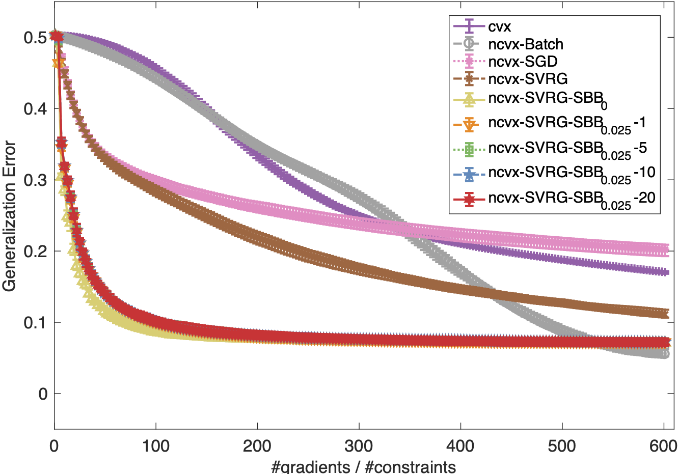
(a) GNMDS

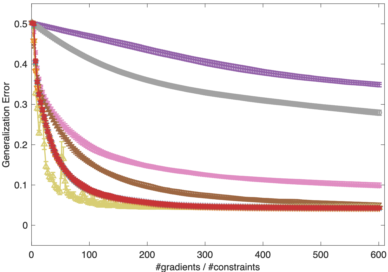
(b) CKL

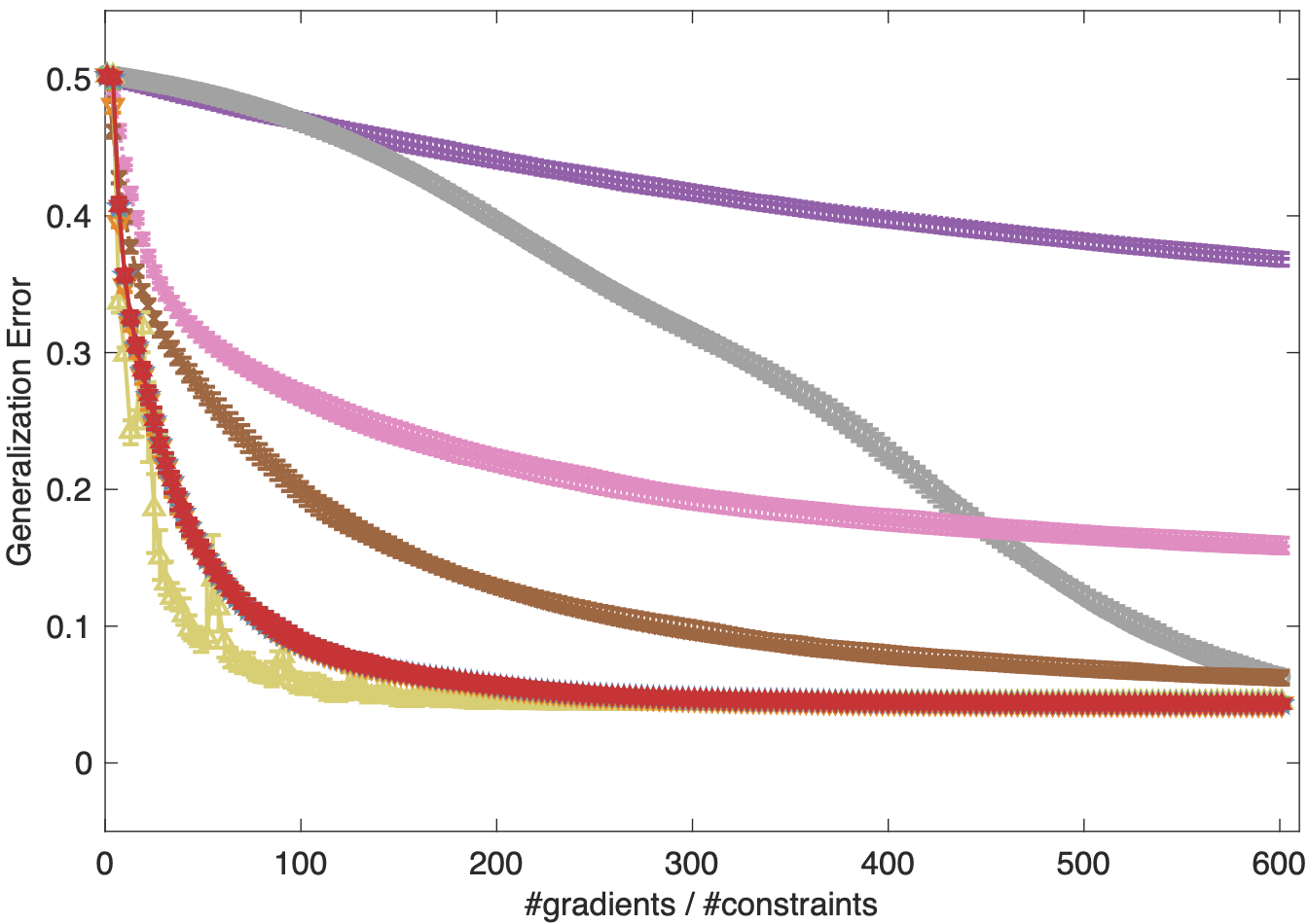
(c) STE

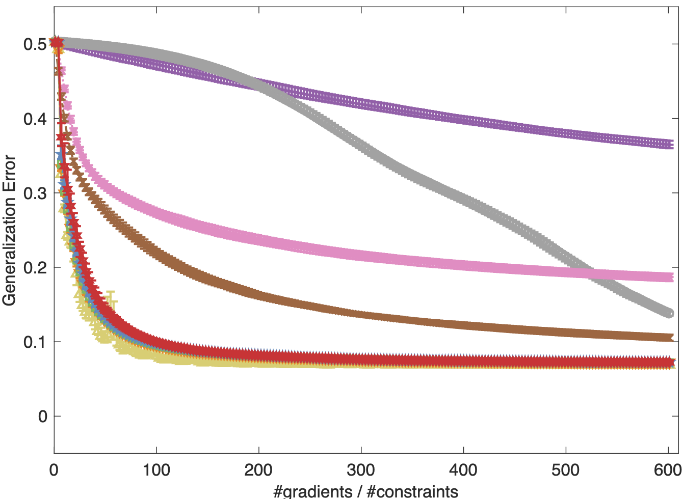
(d) TSTE

Figure 2: Generalization errors of SGD, SVRG, SVRG-SBB and batch methods on the synthetic dataset.

We compare the performance of SVRG-SBB_ϵ and its mini-batch variants with SGD, fixed step size SVRG (called SVRG for short henceforth) as well as the two batch gradient descent methods. We compare these algorithms in the “epoch” sense which means that each method executes the gradient calculation by the same times in every epoch. To be concrete, as SVRG and SVRG-SBB_ϵ evaluate $2m+|\mathcal{Q}|$ times of (sub)gradient in each epoch, the batch and SGD solutions query the same numbers of (sub)gradient. The mini-batch SVRG-SBB_ϵ evaluates $2|\mathcal{I}_{t}|$ gradients in the inner loop where $|\mathcal{I}_{t}|$ is the size of mini-batch. We reduce the inner iteration of the mini-batch SVRG-SBB_ϵ to $m/|\mathcal{I}_{t}|$ for fair comparisons.

Results. In Figure 2, the $x$-axis is the number of gradient calculation divided by the total number of training samples $|\mathcal{Q}|$. We set $m=|\mathcal{Q}|$ for SVRG, SVRG-SBB_ϵ and its min-batch variants. As a consequence, we evaluate the generalization error of each optimization method $3$ times in each epoch. The $y$-axis represents the generalization error. The results are based on $50$ trials with different initialization $\boldsymbol{X}_{0}$. The median of generalization error over $50$ trials with $[0.25,0.75]$ confidence interval are plotted. The whole experiment results, generalization error and the computational complexity are shown in Figure 2 and Table I.

We observe the following phenomena from Figure 2. First of all, due to instability of SBB₀ step size, the SVRG-SBB₀ cause the generalization error to increase. The numerical ‘explosion’ of SBB₀ step size leads to the failure of gradient decent method. This disadvantage of SBB₀ is consistent with our theoretical results and insights. On the other hand, the results of the proposed SBB_ϵ and its mini-batch variant do not vibrate during the whole process. This is the main motivation of the proposed stabilized method. Although the SBB_ϵ method applies the conservative treatment and sacrifices some efficiency, this trade-off is valuable if the objective function does not hold the elegant properties, namely the condition number of Hessian matrix is not too large. Secondly, the SBB_ϵ and its mini-batch variant outperform the SVRG incorporated with fixed step size by clear margins. The SBB_ϵ method can choose more appropriate step size. Thus we can run the algorithm without adding much computational burden by tuning parameter. Just a fixed step size ensures the convergence of non-convex SVRG [31] but this particular step size is related to the Lipschitz constant of the objective function which is hard to obtain in practical problems, especially when the objective functions are non-convex. The SBB_ϵ method is derived from BB step size and the latter one is obtained form the so-called “secant equation” which approximates the inverse of Hessian matrix by the identity matrix multiplied the desired step size. Such an approximation leads to the instability of BB method in stochastic non-convex optimization as the curvature condition (12) does not always hold. A possible future direction is how to preserve the positive-definiteness of the inverse of the Hessian matrix without line search and extremely laborious computation in stochastic paradigm [36]. Moreover, all the stochastic methods including SGD, SVRG and SVRG-SBB_ϵ ($\epsilon=0$ or $\epsilon>0$) converge fast at the initial several epochs and quickly get admissible results in terms of the relatively small generalization error.

Table I shows the computational complexity achieved by batch and stochastic gradient descent with its variants, SGD, SVRR and SVRG-SBB_ϵ for convex and non-convex objective functions. All results are obtained with MATLAB${}^{\text{\textregistered{}}}$ R2016b, on a desktop PC with Windows${}^{\text{\textregistered{}}}$ $7$ SP$1$ $64$ bit, with $3.3$ GHz Intel${}^{\text{\textregistered{}}}$ Xeon${}^{\text{\textregistered{}}}$ E3-1226 v3 CPU, and $32$ GB $1600$ MHz DDR3 memory. It is clear to see that for all objective functions, SVRG-SBB_ϵ ($\epsilon=0$ or $\epsilon>0$) gains speed-up compared to the other methods. The superiority of SVRG-SBB_ϵ mini-batch in terms of the CPU time can also be observed from Table I. Specifically, the speedup of SVRG-SBB_ϵ mini-batch over SVRG is about at least 4 times for all four models.

5.2 Visualization of Eurodist Dataset

The second empirical study is to visualize some objects in $2$d space based on their relative similarity comparisons.

Settings. The “eurodist” dataset describes the “driving” distances (in km) between $21$ cities of Europe, and is available in the stats library of R. In this dataset, there are $21,945$ possible quadruplets (i.e. $(i,j,l,k)$) in total. Here we adopt the “local” setting as only the triplets are utilized where $j=i$. A triplet $(i,j,k)$ represents a partial order as $d^{2}_{ij}<d^{2}_{ik}$, which indicates that “the distance between cities $i$ and $j$ is smaller than the distance between cities $i$ and $k$” and $d^{2}_{ij}$ is the road distance between cities $i$ and $j$ as $i,j\in\{1,...,21\}$. The main task of this dataset is to visualize the embedding of these $21$ cities in $2$-dimensional Euclidean space. We randomly sample $2,000$ triplets as the training set and the left are test set.

(a) Convex Result

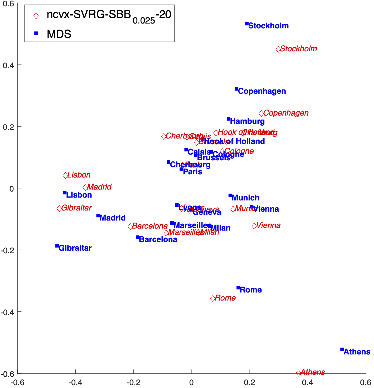
(b) Non-Convex Result

Figure 3: Visualization of the Eurodist dataset.

Competitors. We compare the ordinal embedding results of all four models with the classical metric Multidimensional Scaling (MDS) result. mMDS is also known as Principal Coordinates Analysis (PCoA) or Torgerson–Gower Scaling. It takes an input matrix giving dissimilarities between pairs of objects and outputs a coordinate matrix. Here we employ the road distance between a pair of two cities as their dissimilarities and obtain $2$d coordinates of each cities. Note that there is no perfect embedding in the 2-dimensional space as the given distances are actually geodesic.

Results. Figure 3 displays the Procrustes rotated embedding results of MDS and ordinal embedding. Obviously, the full, explicit distance information helps MDS to gain a better visualization. ODE methods only adopt partial, relative comparisons and their visualizations are inferior to the competitor’s result. However, the non-convex ordinal embedding methods still generate the reasonable representations of these $21$ cities. In the new coordinate system, all the positions are not contrary to geographical knowledge. Furthermore, the stochastic paradigm in SVRG-SBB_ϵ dose not affect the quality of the embedding.

5.3 Music Artists Similarity Comparison

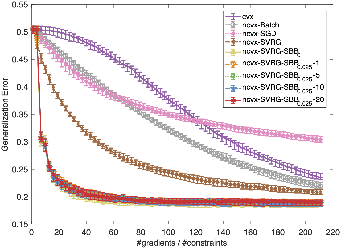
(a) GNMDS

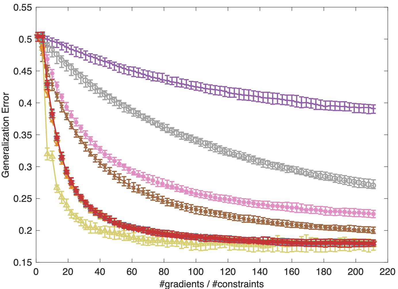
(b) CKL

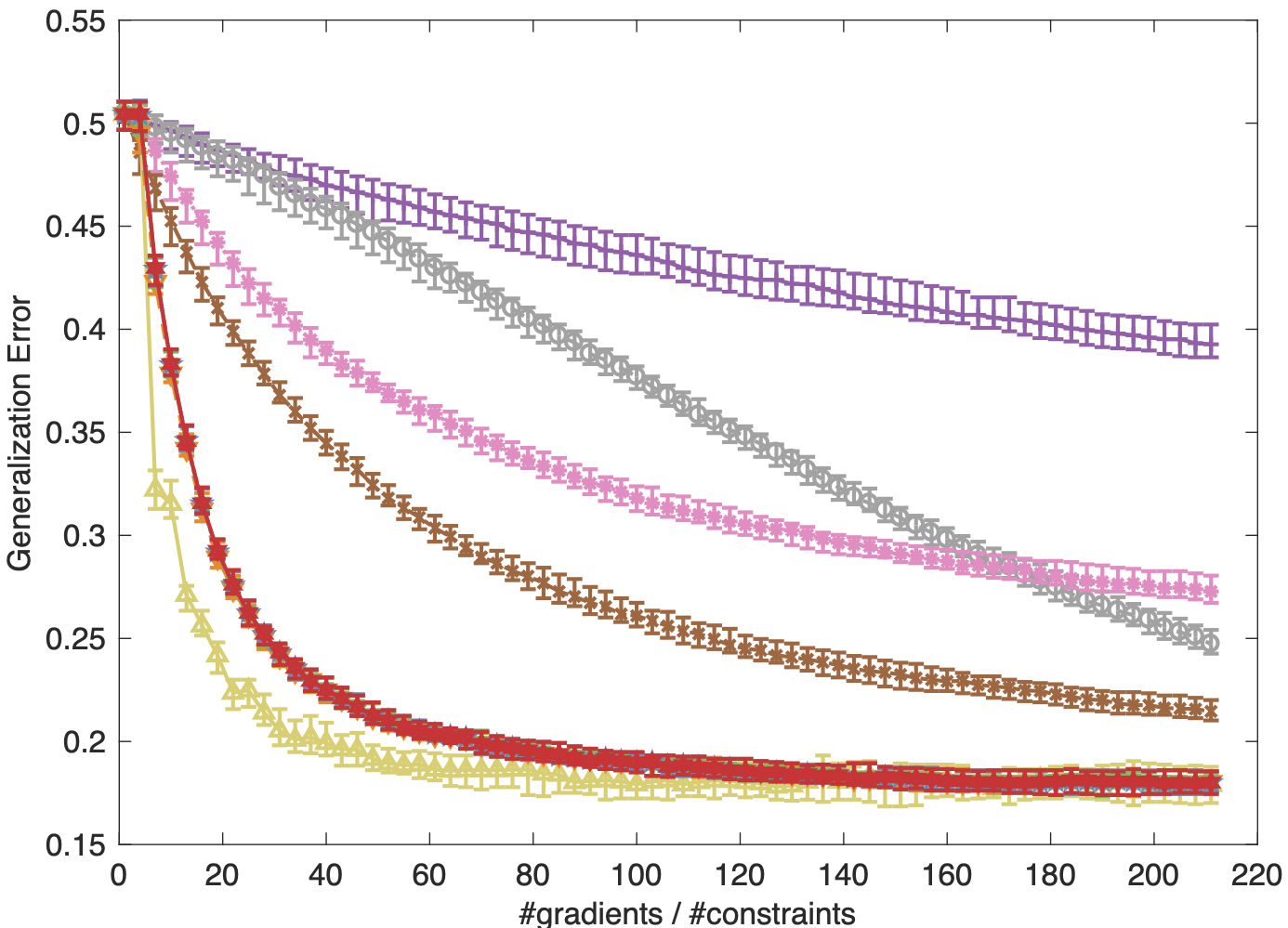
(c) STE

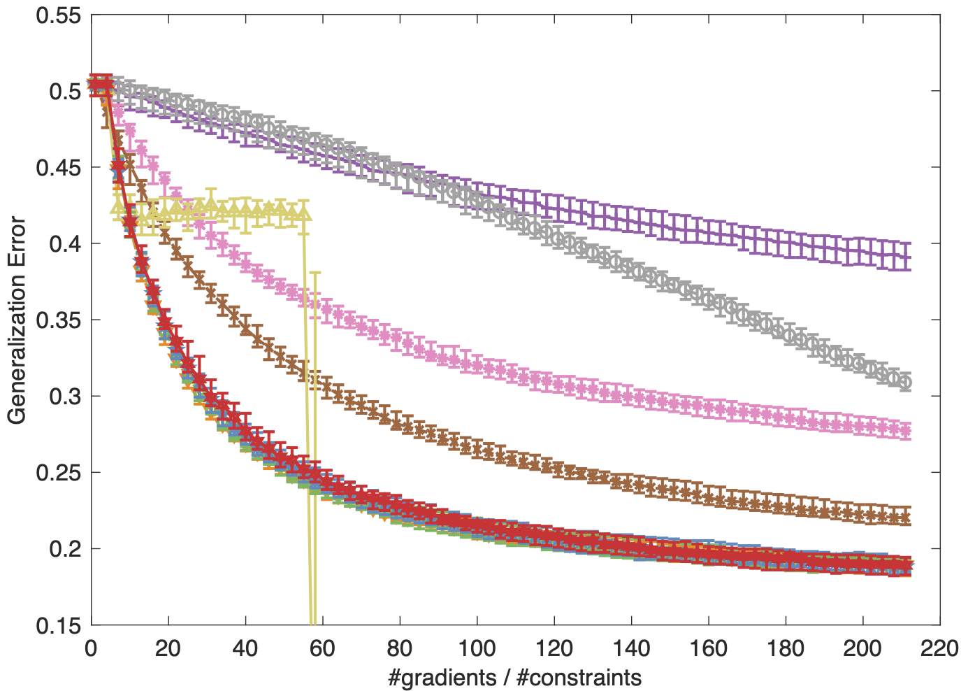
(d) TSTE

Figure 4: Generalization errors of SGD, SVRG, SVRG-SBB and batch methods on the music artists dataset.

We implement all methods on a medium-scale real world dataset, called music artist similarity dataset, which is collected by [37] through a web-based survey.

Settings. In this dataset, there are $412$ music artists involved in triple-wise comparisons based on music genre. The genre labels for all artists are gathered using Wikipedia, to distinguish nine music genres (rock, metal, pop, dance, hip hop, jazz, country, gospel, and reggae). The similarity comparisons are labeled by $1,032$ participants. The number of triplets on the similarity between music artists is $213,472$. A triplet $(i,j,k)$ indicates that “music artist $i$ is more similar to artist $j$ than artist $k$”. Specifically, we use the data pre-processed by [21] via removing the inconsistent triplets from the original dataset. There are $9,107$ triplets for $N=400$ artists. We randomly sample $80$ percent of the comparisons as the training set and the left are the test data. The embedded dimension is $p=9$ as the number of genre category. All methods start with the same initialization $\boldsymbol{X}_{0}$ which is randomly generated.

Results. Each curve in Figure 4 shows the trend of test error of one method with respect to the epoch number. We execute 50 trials of each optimization method for the four objective functions. From Figure 4, SBB_ϵ and its mini-batch variant can significantly speed up SVRG in terms of epoch number. Specially, the test error curves of four SVRG-SBB_ϵ ($\epsilon\geq 0$) methods decay much faster than those of SGD, SVRG and projection gradient descent at the initial epochs. We also observe that the SVRG-SBB₀ tends to failure as the step size is extremely large ($\sim 10^{35}$). The SVRG-SBB_ϵ step size can effectively avoid the occurrence of similar situations.

5.4 Image Retrieval on SUN397

(a) GNMDS

method	5%		10%
	MAP	P	MAP	P
cvx	0.0259	0.0712	0.0255	0.0694
ncvx Batch	0.0474	0.1326	0.0386	0.1119
ncvx SGD	0.3120	0.4606	0.1865	0.3359
ncvx SVRG	0.3460	0.4949	0.2112	0.3631
ncvx SVRG-SBB0	0.4659	0.5783	0.2971	0.4408
ncvx SVRG-SBBϵ-$1$	0.4861	0.5993	0.3085	0.4533
ncvx SVRG-SBBϵ-$5$	0.4861	0.5995	0.3085	0.4536
ncvx SVRG-SBBϵ-$10$	0.4867	0.5998	0.3083	0.4534
ncvx SVRG-SBBϵ-$20$	0.4872	0.6005	0.3085	0.4535

(b) CKL

method	5%		10%
	MAP	P	MAP	P
cvx	0.0258	0.0704	0.0260	0.0711
ncvx Batch	0.0376	0.1087	0.0338	0.0992
ncvx SGD	0.4830	0.5926	0.1765	0.3192
ncvx SVRG	0.5445	0.6450	0.2149	0.3623
ncvx SVRG-SBB0	0.4662	0.5793	0.2037	0.3547
ncvx SVRG-SBBϵ-$1$	0.5645	0.6525	0.2805	0.4270
ncvx SVRG-SBBϵ-$5$	0.5652	0.6532	0.2809	0.4273
ncvx SVRG-SBBϵ-$10$	0.5653	0.6533	0.2810	0.4274
ncvx SVRG-SBBϵ-$20$	0.5653	0.6533	0.2810	0.4274

(c) STE

method	5%		10%
	MAP	P	MAP	P
cvx	0.0257	0.0707	0.0262	0.0722
ncvx Batch	0.0304	0.0881	0.0306	0.0874
ncvx SGD	0.2820	0.4261	0.1948	0.3391
ncvx SVRG	0.5265	0.6302	0.3783	0.5105
ncvx SVRG-SBB0	0.4637	0.5799	0.0070	0.0555
ncvx SVRG-SBBϵ-$1$	0.6387	0.7147	0.4584	0.5730
ncvx SVRG-SBBϵ-$5$	0.6362	0.7129	0.4568	0.5719
ncvx SVRG-SBBϵ-$10$	0.6359	0.7127	0.4566	0.5719
ncvx SVRG-SBBϵ-$20$	0.6358	0.7126	0.4565	0.5717

(d) TSTE

method	5%		10%
	MAP	P	MAP	P
cvx	0.0257	0.0695	0.0261	0.0704
ncvx Batch	0.0270	0.0736	0.0273	0.0751
ncvx SGD	0.3864	0.5074	0.2381	0.3742
ncvx SVRG	0.7198	0.7746	0.5241	0.6221
ncvx SVRG-SBB0	0.0070	0.0555	0.0070	0.0555
ncvx SVRG-SBBϵ-$1$	0.8861	0.9034	0.6859	0.7431
ncvx SVRG-SBBϵ-$5$	0.8898	0.9030	0.6865	0.7437
ncvx SVRG-SBBϵ-$10$	0.8866	0.9000	0.6854	0.7432
ncvx SVRG-SBBϵ-$20$	0.8846	0.8995	0.6847	0.7426

TABLE II: Image retrieval performance (MAP and Precision@60) on SUN397

We apply the ordinal embedding method with the proposed SVRG-SBB algorithm on a real-world dataset, i.e., SUN 397. In the visual search task, we wish to see how the learned representation or embedding characterizes the “relevance” of the same image category and the “discrimination” of different image categories. Hence, we use the image representation obtained by ordinal embedding for image retrieval.

Settings. We evaluate the effectiveness of the ordinal embedding methods for image retrieval on the SUN$397$ dataset. SUN$397$ consists of about $108,000$ images from $397$ scene categories. In SUN$397$, each image has a $1,600$-dimensional feature vector extracted by principle component analysis (PCA) from $12,288$-dimensional Deep Convolution Activation Features [38]. We form the training set by randomly sampling $1,080$ images from $18$ categories with $60$ images in each category. Only the training set is used for learning the representations from ordinal constraints and a nonlinear mapping from the original feature space to the embedded space. We denote the mapping as $\mathcal{M}:\mathbb{R}^{1600}\rightarrow\mathbb{R}^{18}$. The nonlinear mapping $\mathcal{M}$ is used to predict the embedded images in $\mathbb{R}^{18}$, which do not participate in the relative similarity comparisons. We use Regularized Least Square (RLS) and RBF kernel to solve the nonlinear mapping $\mathcal{M}$. The test set consists of $720$ images randomly chosen from $18$ categories with $40$ images in each category. We use labels of training images to generate the similarity comparisons. The ordinal constraints are generated like [16]: we randomly sample two images $i,\ j$ which are from the same category and choose image $k$ from the left categories. As the semantic similarity between $i$ and $j$ in the same class is larger than the similarity between $i$ and $k$ in the different class, a triplet $(i,j,k)$ describes the relative similarity comparison. The total number of such triplets is $70,000$. Wrong triplets are then synthesized to simulate the human error in real-world data. We randomly sample $5\%,10\%$ and $15\%$ triplets to exchange the positions of $j$ and $k$ in each triplet $(i,j,k)$.

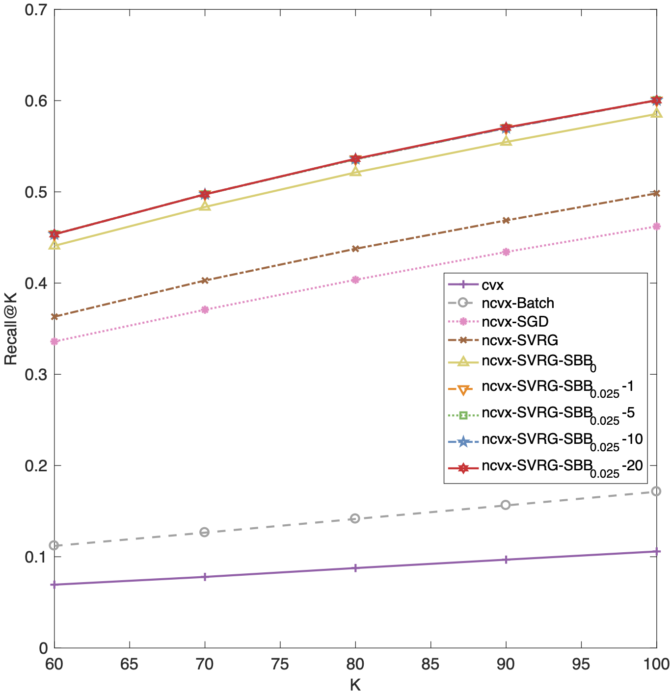
(a) GNMDS

(b) CKL

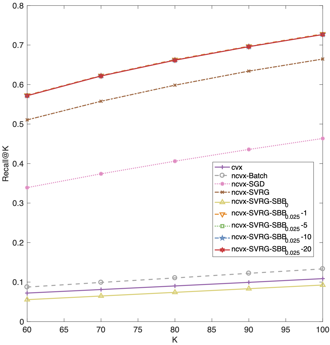
(c) STE

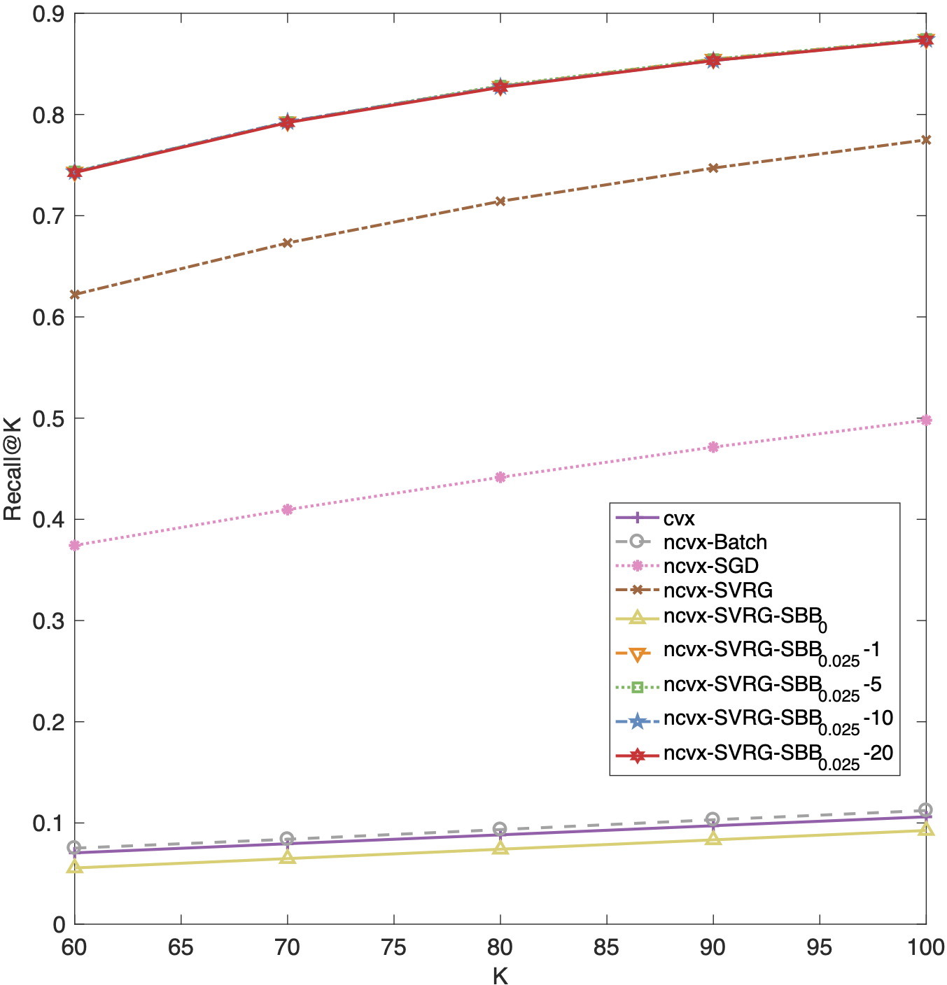
(d) TSTE

Figure 5: Recall@K with $10\%$ noise on SUN397.

Evaluation Metrics. To measure the effectiveness of various ordinal embedding methods for visual search, we consider three evaluation metrics, i.e., precision at top-K positions (Precision@K), recall at top-K positions (Recall@K), and Mean Average Precision (MAP). Given the mapped feature $\boldsymbol{X}=\{\boldsymbol{x}_{1},\boldsymbol{x}_{2},\dots,\boldsymbol{x}_{720}\}\subset\mathbb{R}^{18}$ of test images and an image $i\in[n]$ belonging to the class $c_{i}$ as a query, we sort the images of training set according to the distances between their embedded feature in $\mathbb{R}^{18}$ and $\boldsymbol{x}_{i}$ in an ascending order as $\mathcal{R}_{i}$. True positives ($\textit{TP}^{K}_{i}$) are images correctly labeled as positives, which involve the images belonging to $c_{i}$ and listed within the top K positions in $\mathcal{R}_{i}$. False positives ($\text{FP}^{K}_{i}$) refer to negative examples incorrectly labeled as positives, which are the images belonging to $c_{l}(l\neq i)$ and listed within the top K in $\mathcal{R}_{i}$. True negatives ($\text{TN}^{K}_{i}$) correspond to negatives correctly labeled as negatives, which refer to the images belonging to $c_{l}(l\neq i)$ and listed after the top K in $\mathcal{R}_{i}$. Finally, false negatives ($\text{FN}^{K}_{i}$) refer to positive examples incorrectly labeled as negatives, which are relevant to the images belonging to class $c_{i}$ and listed after the top K in $\mathcal{R}_{i}$. We are able to define Precision@K and Recall@K as: $\text{Precision@}K=\frac{1}{n}\sum_{i}^{n}p_{i}^{K}=\frac{1}{n}\sum_{i}^{n}\frac{\text{TP}^{K}_{i}}{\text{TP}^{K}_{i}+\text{FP}^{K}_{i}}$ and $\text{Recall@}K=\frac{1}{n}\sum_{i}^{n}r_{i}^{K}=\frac{1}{n}\sum_{i}^{n}\frac{\text{TP}^{K}_{i}}{\text{TP}^{K}_{i}+\text{FN}^{K}_{i}}.$ These two measurements are both single-valued metric based on the top K ranking order of training images refered to the query image. It is also desirable to consider the total order of the training images which are in the same category as the query image. By computing precision and recall at every position in the ranked sequence for query $\boldsymbol{x}_{i}$, one can plot a precision-recall curve, plotting precision $p_{i}(r)$ as a function of recall $r_{i}$. Average Precision (AP) computes the average value of $p_{i}(r)$ over the interval from $r_{i}=0$ to $r_{i}=1$: $\text{AP}_{i}=\int_{0}^{1}p_{i}(r_{i})dr_{i},$ which is the area under precision-recall curve. This integral can be replaced with a finite sum over every position $s$ in the ranked sequence of the embedding: $\text{AP}_{i}=\sum_{s=1}^{40}p_{i}(s)\cdot\triangle r_{i}(s),$ where $\triangle r_{i}(s)$ is the change in recall from items $s-1$ to $s$. The MAP used in this paper is defined as $\text{MAP}=\frac{1}{n}\sum_{i=1}^{n}\text{AP}_{i}$.

Results. The experiment results are shown in Table II and Figure 5. With $K$ varying from $40$ to $100$, we observe that non-convex SVRG-SBB_ϵ consistently achieves the superior Precision@K, Recall@K and MAP results against the other methods with the same gradient calculation. The results illustrate that SVRG-SBB_ϵ is more suitable for non-convex objective functions than SVRG-SBB₀. SVRG-SBB_ϵ has a very promising potential in practice, because it generates appropriate step sizes automatically while running the algorithm and the result is robust. Moreover, under our setting, all the ordinal embedding methods achieve reasonable results for image retrieval. It illustrates that high-quality relative similarity comparisons can be used for learning meaningful representation of massive data, thereby making it easier to extract useful information in other applications.

6 Conclusions

In this paper, we propose a stochastic non-convex framework for the ordinal embedding problem. A novel stochastic gradient descent algorithm called SVRG-SBB is applied to solve this non-convex formulation. The proposed SVRG-SBB is a variant of SVRG method. It incorporate with the so-called stabilized BB (SBB) step size, a new, stable and adaptive step size introduced in this paper. The motivation of the SBB step size is to overcome the instability of the original BB step size when the strongly convexity is absent. We also establish the $O(1/T)$ convergence rate of SVRG-SBB. Such a convergence rate is comparable to the existing best convergence results of SVRG in the literature. Furthermore, we derive the analysis to mini-batch variants of SVRG-SBB. We also analyze the PL function on which SVRG-SBB attains linear convergence to the global optimum. A series of simulations and real-world data experiments are implemented to demonstrate the effectiveness of the proposed SVRG-SBB for the ordinal embedding problem. The proposed SVRG-SBB outperforms most of the state-of-the-art methods from the perspective of computational cost.

A. Proof of Lemma 1

To prove Lemma 1, we need the following lemma, which establishes the bound of the norm of variance gradient ${\boldsymbol{u}}_{t}^{s+1}$.

Lemma 2 (Bounded $\mathbb{E}\left(\|{\boldsymbol{u}}_{t}^{s+1}\|^{2}\right)$).

Under assumptions of Lemma 1, the following holds

$$\mathbb{E}\left[\left\|\boldsymbol{x}_{t}^{s+1}\right\|^{2}\right]\leq 2\mathbb{E}\left[\left\|\nabla f(\boldsymbol{x}_{t}^{s+1})\right\|^{2}\right]+\frac{2L^{2}}{b}\mathbb{E}\left[\left\|\boldsymbol{x}_{t}^{s+1}-\tilde{\boldsymbol{x}}^{s}\right\|^{2}\right].$$

Proof.

Let $\boldsymbol{v}_{t}^{s+1}:=\frac{1}{b}\sum_{i_{t}\in{\cal I}_{t}}\left(\nabla f_{i_{t}}\left(\boldsymbol{x}_{t}^{s+1}\right)-\nabla f_{i_{t}}\left(\tilde{\boldsymbol{x}}^{s}\right)\right)$, then $\boldsymbol{u}_{t}^{s+1}={\boldsymbol{v}}_{t}^{s+1}+\nabla f\left(\tilde{\boldsymbol{x}}^{s}\right)$. Thus,

$$\mathbb{E}\left[\left\|{\boldsymbol{u}}_{t}^{s+1}\right\|^{2}\right] = \ \ \ \ \mathbb{E}\left[\left\|{\boldsymbol{v}}_{t}^{s+1}-\left(\nabla f\left({\boldsymbol{x}}_{t}^{s+1}\right)-\nabla f\left(\tilde{\boldsymbol{x}}^{s}\right)\right)+\nabla f\left(\boldsymbol{x}_{t}^{s+1}\right)\right\|^{2}\right]$$

$$\leq \ \ \ \ 2\mathbb{E}\left[\left\|\nabla f(\boldsymbol{x}_{t}^{s+1})\right\|^{2}\right]+2\mathbb{E}\left[\left\|{\boldsymbol{v}}_{t}^{s+1}-\mathbb{E}\left[{\boldsymbol{v}}_{t}^{s+1}\right]\right\|^{2}\right]$$

$$= \ \ \ \ 2\mathbb{E}\left[\left\|\nabla f\left({\boldsymbol{x}}_{t}^{s+1}\right)\right\|^{2}\right]+\frac{2}{b^{2}}\mathbb{E}\left[\left\|\sum_{i_{t}\in{\cal I}_{t}}\left(\nabla f_{i_{t}}\left({\boldsymbol{x}}_{t}^{s+1}\right)-\nabla f_{i_{t}}\left(\tilde{\boldsymbol{x}}^{s}\right)-\mathbb{E}\left({\boldsymbol{v}}_{t}^{s+1}\right)\right)\right\|^{2}\right]$$

$$\leq \ \ \ \ 2\mathbb{E}\left[\left\|\nabla f\left({\boldsymbol{x}}_{t}^{s+1}\right)\right\|^{2}\right]+\frac{2}{b}\mathbb{E}\left[\left\|\nabla f_{i_{t}}\left({\boldsymbol{x}}_{t}^{s+1}\right)-\nabla f_{i_{t}}\left(\tilde{\boldsymbol{x}}^{s}\right)\right\|^{2}\right]$$

$$\leq \ \ \ \ 2\mathbb{E}\left[\left\|\nabla f\left({\boldsymbol{x}}_{t}^{s+1}\right)\right\|^{2}\right]+\frac{2L^{2}}{b}\mathbb{E}\left[\left\|{\boldsymbol{x}}_{t}^{s+1}-\tilde{\boldsymbol{x}}^{s}\right\|^{2}\right],$$

where the first inequality holds for the basic inequality, i.e., $\|\boldsymbol{a}+\boldsymbol{b}\|^{2}\leq 2(\|\boldsymbol{a}\|^{2}+\|\boldsymbol{b}\|^{2})$ for any two vectors of the same sizes, the second inequality holds for the fact that $i_{t}$ are drawn uniformly randomly and independently from $\{1,2,\ldots,n\}$ and noting that for a random variable $\xi$, $\mathbb{E}[\|\xi-\mathbb{E}[\xi]\|^{2}]\leq\mathbb{E}[\|\xi\|^{2}]$, and the final inequality holds for the $L$-smoothness of $f_{i_{t}}$. ∎

Based on this lemma, we prove Lemma 1 as follows.

Proof of Lemma 1.

By the $L$-smoothness of each $f_{i}$ (implying the $L$-smoothness of $f$), there holds

$$\mathbb{E}\left[f\left({\boldsymbol{x}}_{t+1}^{s+1}\right)\right] \leq \ \ \ \mathbb{E}\left[f\left({\boldsymbol{x}}_{t}^{s+1}\right)\right]+\frac{L}{2}\mathbb{E}\left[\left\|{\boldsymbol{x}}_{t+1}^{s+1}-{\boldsymbol{x}}_{t}^{s+1}\right\|^{2}\right]+\mathbb{E}\left[\left\langle\nabla f\left({\boldsymbol{x}}_{t}^{s+1}\right),\ {\boldsymbol{x}}_{t+1}^{s+1}-{\boldsymbol{x}}_{t}^{s+1}\right\rangle\right]$$

$$= \ \ \ \mathbb{E}\left[f\left({\boldsymbol{x}}_{t}^{s+1}\right)\right]-b\eta_{\epsilon,s}\mathbb{E}\left[\left\|\nabla f\left({\boldsymbol{x}}_{t}^{s+1}\right)\right\|^{2}\right]+\frac{Lb^{2}\eta_{\epsilon,s}^{2}}{2}\mathbb{E}\left[\left\|{\boldsymbol{x}}_{t}^{s+1}\right\|^{2}\right],$$

where the equality holds for

$$\mathbb{E}\left[\langle\nabla f\left({\boldsymbol{x}}_{t}^{s+1}\right),{\boldsymbol{x}}_{t+1}^{s+1}-{\boldsymbol{x}}_{t}^{s+1}\rangle\right]=-b\eta_{\epsilon,s}\mathbb{E}\left[\left\langle\nabla f\left({\boldsymbol{x}}_{t}^{s+1}\right),\mathbb{E}\left[{\boldsymbol{x}}_{t}^{s+1}\right]\right\rangle\right]=-b\eta_{\epsilon,s}\mathbb{E}\left[\left\|\nabla f\left({\boldsymbol{x}}_{t}^{s+1}\right)\right\|^{2}\right].$$

Moreover, note that

$$\mathbb{E}\left[\left\|{\boldsymbol{x}}_{t+1}^{s+1}-\tilde{\boldsymbol{x}}^{s}\right\|^{2}\right] = \ \ \ \mathbb{E}\left[\left\|{\boldsymbol{x}}_{t+1}^{s+1}-{\boldsymbol{x}}_{t}^{s+1}+{\boldsymbol{x}}_{t}^{s+1}-\tilde{\boldsymbol{x}}^{s}\right\|^{2}\right]$$

$$= \ \ \ \mathbb{E}\left[\left\|{\boldsymbol{x}}_{t+1}^{s+1}-{\boldsymbol{x}}_{t}^{s+1}\right\|^{2}\right]+\mathbb{E}\left[\left\|{\boldsymbol{x}}_{t}^{s+1}-\tilde{\boldsymbol{x}}^{s}\right\|^{2}\right]+2\mathbb{E}\left[\left\langle{\boldsymbol{x}}_{t+1}^{s+1}-{\boldsymbol{x}}_{t}^{s+1},{\boldsymbol{x}}_{t}^{s+1}-\tilde{\boldsymbol{x}}^{s}\right\rangle\right]$$

$$= \ \ \ \mathbb{E}\left[\left\|{\boldsymbol{x}}_{t}^{s+1}-\tilde{\boldsymbol{x}}^{s}\right\|^{2}\right]+b^{2}\eta^{2}_{\epsilon,s}\mathbb{E}\left[\left\|{\boldsymbol{u}}_{t}^{s+1}\right\|^{2}\right]-2b\eta_{\epsilon,s}\mathbb{E}\left[\left\langle\nabla f\left({\boldsymbol{x}}_{t}^{s+1}\right),{\boldsymbol{x}}_{t}^{s+1}-\tilde{\boldsymbol{x}}^{s}\right\rangle\right]$$

$$\leq \ \ \ \mathbb{E}\left[\left\|{\boldsymbol{x}}_{t}^{s+1}-\tilde{\boldsymbol{x}}^{s}\right\|^{2}\right]+b^{2}\eta^{2}_{\epsilon,s}\mathbb{E}\left[\left\|{\boldsymbol{u}}_{t}^{s+1}\right\|^{2}\right]+2b\eta_{\epsilon,s}\left[\frac{1}{2\beta_{s}}\mathbb{E}\left[\left\|\nabla f({\boldsymbol{x}}_{t}^{s+1})\right\|^{2}\right]+\frac{\beta_{s}}{2}\left\|{\boldsymbol{x}}_{t}^{s+1}-\tilde{\boldsymbol{x}}^{s}\right\|^{2}\right]$$

$$= \ \ \ \left(1+b\eta_{\epsilon,s}\beta_{s}\right)\mathbb{E}\left[\left\|{\boldsymbol{x}}_{t}^{s+1}-\tilde{\boldsymbol{x}}^{s}\right\|^{2}\right]+b\eta_{\epsilon,s}\beta_{s}^{-1}\mathbb{E}\left[\left\|\nabla f({\boldsymbol{x}}_{t}^{s+1})\right\|^{2}\right]+b^{2}\eta^{2}_{\epsilon,s}\mathbb{E}\left[\left\|{\boldsymbol{u}}_{t}^{s+1}\right\|^{2}\right],$$

where the third equality holds for the iterate of the proposed SVRG method, i.e., ${\boldsymbol{x}}_{t+1}^{s+1}={\boldsymbol{x}}_{t}^{s+1}-b\eta_{\epsilon,s}{\boldsymbol{u}}_{t}^{s+1}$, and the inequality holds for the Young’s inequality with some positive constant $\beta_{s}$.

Now consider the Lyapunov function

$$R_{t,s+1}:=\mathbb{E}\left[f\left({\boldsymbol{x}}_{t}^{s+1}\right)\right]+c_{t,s}\mathbb{E}\left[\left\|{\boldsymbol{x}}_{t}^{s+1}-\tilde{\boldsymbol{x}}^{s}\right\|^{2}\right],$$

where $c_{t,s}$ is specified in (20). By (Proof of Lemma 1.) and (Proof of Lemma 1.), there holds

$$R_{t+1,s+1} \leq \ \ \ \left(1+b\eta_{\epsilon,s}\beta_{s}\right)c_{t+1,s}\mathbb{E}\left[\left\|{\boldsymbol{x}}_{t}^{s+1}-\tilde{\boldsymbol{x}}_{s}\right\|^{2}\right]-b\eta_{\epsilon,s}\left(1-c_{t+1,s}\beta_{s}^{-1}\right)\mathbb{E}\left[\left\|\nabla f\left({\boldsymbol{x}}_{t}^{s+1}\right)\right\|^{2}\right]$$

$$\ \ \ +b^{2}\eta^{2}_{\epsilon,s}\left(c_{t+1,s}+\frac{L}{2}\right)\mathbb{E}\left[\left\|{\boldsymbol{u}}_{t}^{s+1}\right\|^{2}\right]+\mathbb{E}\left[f\left({\boldsymbol{x}}_{t}^{s+1}\right)\right].$$

Plugging the bound of $\mathbb{E}\left[\left\|u_{t}^{s+1}\right\|^{2}\right]$ established in Lemma 2 into the above inequality yields

$$R_{t+1,s+1}\leq\mathbb{E}\left[f\left({\boldsymbol{x}}_{t}^{s+1}\right)\right]+c_{t,s}\mathbb{E}\left[\left\|{\boldsymbol{x}}_{t}^{s+1}-\tilde{\boldsymbol{x}}^{s}\right\|^{2}\right]-b\eta_{\epsilon,s}\left[1-\frac{c_{t+1,s}}{\beta_{s}}-2b\eta_{\epsilon,s}\left(c_{t+1,s}+\frac{L}{2}\right)\right]\mathbb{E}\left[\left\|\nabla f\left({\boldsymbol{x}}_{t}^{s+1}\right)\right\|^{2}\right],$$

which concludes this lemma via the definition of $\Gamma_{t,s}$ (21). ∎

B. Proof of Theorem 1

Proof.

By Lemma 1, for any $0\leq s\leq S-1$,

$$\sum_{t=0}^{m-1}\mathbb{E}\left[\left\|\nabla f\left({\boldsymbol{x}}_{t}^{s+1}\right)\right\|^{2}\right]\leq\frac{R_{0,s+1}-R_{m,s+1}}{\gamma_{S}}.$$

Noting that ${\boldsymbol{x}}_{0}^{s+1}=\tilde{\boldsymbol{x}}^{s}$, ${\boldsymbol{x}}_{m}^{s+1}=\tilde{\boldsymbol{x}}^{s+1}$ and $c_{m,s}=0$, the above inequality implies

$$\sum_{t=0}^{m-1}\mathbb{E}\left[\left\|\nabla f\left({\boldsymbol{x}}_{t}^{s+1}\right)\right\|^{2}\right]\leq\frac{\mathbb{E}\left[f\left(\tilde{\boldsymbol{x}}^{s}\right)\right]-\mathbb{E}\left[f\left(\tilde{\boldsymbol{x}}^{s+1}\right)\right]}{\gamma_{S}}.$$

Summing over $s$ from $0$ to $S-1$, the above inequality yields

$$\frac{1}{mS}\sum_{s=0}^{S-1}\sum_{t=0}^{m-1}\mathbb{E}\left[\left\|\nabla f\left({\boldsymbol{x}}_{t}^{s+1}\right)\right\|^{2}\right]\leq\frac{f\left(\tilde{\boldsymbol{x}}^{0}\right)-f\left({\boldsymbol{x}}^{*}\right)}{mS\gamma_{S}}.$$

Using the above inequality and the definition of ${\boldsymbol{x}}_{\mathrm{out}}$ in Algorithm 1, we conclude this theorem. ∎

C. Proof of Theorem 2

To prove this theorem, we need the following lemma.

Lemma 3.

Given some positive integer $l\geq 2$, then for any $0<x\leq\frac{1}{l}$, the following holds $(1+x)^{l}\leq e^{lx}\leq 1+2lx$.

Proof.

Note that $(1+x)^{l}=e^{l\cdot\ln(1+x)}\leq e^{lx}$,where the last inequality holds for $\ln(1+x)\leq x$ for any $x\in(0,1]$. Thus, we get the first inequality. Let $h(z)=1+2z-e^{z}$ for any $z\in(0,1]$. It is easy to check that $h(z)\geq 0$ for any $z\in(0,1]$. Thus we get the second inequality. ∎

Based on this lemma, we show the proof of Theorem 2.

Proof of Theorem 2.

To prove this theorem, it only suffices to show that (22) holds under the choice of $\beta_{s}$ (23) and condition (24) presented in this theorem. To achieve this, we first provide two intermediate conditions implying (22),

$$b\eta_{\epsilon,s}\beta_{s}+2b\eta_{\epsilon,s}^{s}L^{2}\leq\frac{1}{m},$$ (29)

$$b\eta_{\epsilon,s}\beta_{s}+b\eta_{\epsilon,s}L<\frac{1}{2},$$ (30)

and then show that (24) together with the choice of $\beta_{s}$ (23) imply (29)-(30).

(a) Here, we prove that (29) and (30) implies (22). According to (20) and the initial condition ${c}_{m,s}=0$, we can easily check that for $t=m-1,\ldots,1,$

$$c_{t,s}=\frac{(\left(\rho_{s}\right)^{m-t}-1)\eta_{\epsilon,s}L^{3}}{\beta_{s}+2\eta_{\epsilon,s}L^{2}}.$$

Noting that $\rho_{s}>1$ by its definition (19), then for any $t=1,\ldots,m-1$,

$$c_{t,s}\leq c_{1,s}<\frac{(\left(\rho_{s}\right)^{m}-1)\eta_{\epsilon,s}L^{3}}{\beta_{s}+2\eta_{\epsilon,s}L^{2}}.$$ (31)

By (29) and Lemma 3,

$$(\rho_{s})^{m} =\left(1+b\eta_{\epsilon,s}\beta_{s}+2b\eta_{\epsilon,s}^{2}L^{2}\right)^{m}$$

$$\leq 1+2mb\eta_{\epsilon,s}(\beta_{s}+2\eta_{\epsilon,s}L^{2}).$$ (32)

Plugging (32) into (31), and by the definition of (23) imply

$$c_{t,s}<\frac{1}{2}\beta_{s},\ t=1,\ldots,m,\ s=0,\ldots,S-1.$$ (33)

By (33) and (30), there holds

$$b\eta_{\epsilon,s}(L+2c_{t+1,s})+c_{t+1,s}\beta_{s}^{-1}<b\eta_{\epsilon,s}(L+\beta_{s})+1/2<1.$$

This yields (22).

(b) In the next, we show that (24) implies (29) and (30). By the definition of $\eta_{\epsilon,s}$ (17) and the $L$-smoothness of $f$, there holds

$$\frac{1}{mL}<\eta_{\epsilon,s}<\frac{1}{m\epsilon}.$$ (34)

Note that

$$b\eta_{\epsilon,s}\beta_{s}+2b\eta^{2}_{\epsilon,s}L^{2}=4mb^{2}\eta_{\epsilon,s}^{3}L^{3}+2b\eta_{\epsilon,s}^{2}L^{2}\leq\frac{1}{m}\left[\frac{4L^{3}}{\epsilon^{3}}\cdot\left(\frac{b}{m}\right)^{2}+\frac{2L^{2}}{\epsilon^{2}}\cdot\frac{b}{m}\right]<\frac{1}{m},$$

where the first inequality holds for (34), and the final inequality follows from (24) (i.e., $\frac{b}{m}<\frac{\epsilon^{2}}{L^{2}\left(1+\sqrt{1+4\epsilon L^{-1}}\right)}$). The above inequality yields (29). Similarly, note that

$$\ \ b\eta_{\epsilon,s}\beta_{s}+b\eta_{\epsilon,s}L=4mb^{2}\eta_{\epsilon,s}^{3}L^{3}+b\eta_{\epsilon,s}L\leq\frac{4L^{3}}{\epsilon^{3}}\cdot\left(\frac{b}{m}\right)^{2}+\frac{L}{\epsilon}\cdot\left(\frac{b}{m}\right)<\frac{1}{4}<\frac{1}{2},$$ (35)

where the first inequality holds for (34), and the final inequality follows from (24) (i.e., $b/m<\epsilon/2L(1+\sqrt{4L/\epsilon+1})$). The above inequality implies (30).

Furthermore, by (33) and the definitions of $\Gamma_{t,s}$ (21) and $\beta_{s}$ (23), there holds

$$\Gamma_{t,s}\geq b\eta_{\epsilon,s}\left[\frac{1}{2}-b\eta_{\epsilon,s}(L+\beta_{s})\right]\geq\frac{1}{4}b\eta_{\epsilon,s},$$

where the second inequality follows from (35). Thus,

$$\gamma_{S}:=\min_{1\leq t\leq m,0\leq s\leq S-1}\Gamma_{t,s} \geq\frac{1}{4}b\min_{0\leq s\leq S-1}\eta_{\epsilon,s}.$$

By Theorem 1, we conclude (25). ∎

D. Proof of Theorem 3

Proof.

According to Theorem 2, the following holds begin

$$\mathbb{E}[\|\nabla f(\tilde{{\boldsymbol{x}}}^{k})\|^{2}]\leq\frac{4\mathbb{E}[f(\tilde{{\boldsymbol{x}}}^{k-1})-f({\boldsymbol{x}}^{*})]}{mSb\eta_{\epsilon,\min}}\leq\frac{2\mathbb{E}[\|\nabla f(\tilde{\boldsymbol{x}}^{k-1})\|^{2}]}{\lambda mSb\eta_{\epsilon,\min}}\leq\rho\mathbb{E}[\|\nabla f(\tilde{\boldsymbol{x}}^{k-1})\|^{2}]$$ (36)

where the second inequality holds for the PL property. The above inequality implies (27). By the PL property of $f$ again, we have

$$\mathbb{E}[\|\nabla f(\tilde{{\boldsymbol{x}}}^{k})\|^{2}]\geq 2\lambda\mathbb{E}[f(\tilde{{\boldsymbol{x}}}^{k})-f({\boldsymbol{x}}^{*})].$$

This together with (36) yields (28). ∎

Next, we provide some details including the convex and non-convex formulation of GOE, some discussion of the GOE framework and the proof for the lemma, propositions and theorems we proposed in the main paper. The numbering of equations and the reference follows that of the main paper.

E. Convex and Non-convex Formulation of GOE

First, we revise some existing classification based ordinal embedding methods and verify that they are all the specific cases of generalized ordinal embedding (5). As the dissimilarity functions in these method are all adopted as the squared Euclidean distance $\|\cdot\|^{2}_{2}$, we adopt the matrix $\boldsymbol{X}\in\mathbb{R}^{p\times n}$ to represent the embedding $\mathcal{X}$ for description clarity.

First of all, we introduce the Gram matrix $\boldsymbol{G}$ to linearize the distance calculation. We assume the matrix $\boldsymbol{X}=\{\boldsymbol{x}_{1},\dots,\boldsymbol{x}_{n}\}\in\mathbb{R}^{p\times n}$ is centered at the origin as

$$\sum_{i=1}^{n}\ \boldsymbol{x}_{i}=\boldsymbol{0},$$ (37)

and define the centering matrix $\boldsymbol{C}$

$$\boldsymbol{C}=\boldsymbol{I}-\frac{1}{n}\boldsymbol{1}\cdot\boldsymbol{1}^{\top},$$ (38)

where $\boldsymbol{1}$ is a $n$-dimensional all-one column vector. With (37), we immediately have $\boldsymbol{XC}=\boldsymbol{X}$. We call the Gram matrix $\boldsymbol{G}=\boldsymbol{X}^{\top}\boldsymbol{X}$ is also “centered” if $\boldsymbol{X}$ is a centered matrix which satisfies (37), and it holds that

$$\boldsymbol{G}=\boldsymbol{X}^{\top}\boldsymbol{X}=\boldsymbol{C}^{\top}\boldsymbol{X}^{\top}\boldsymbol{XC}=\boldsymbol{C}^{\top}\boldsymbol{GC}.\\$$ (39)

Given a centered matrix $\boldsymbol{X}$, we can establish a bijection between the Gram matrix $\boldsymbol{G}$ and the squared Euclidean distance matrix $\boldsymbol{D}$ as

$$\boldsymbol{G}\ =\ -\frac{1}{2}\boldsymbol{CDC},$$ (40a)

$$\boldsymbol{D}\ =\ \textit{diag}(\boldsymbol{G})\cdot\boldsymbol{1}^{\top}-2\boldsymbol{G}+\boldsymbol{1}\cdot\textit{diag}(\boldsymbol{G})^{\top},$$ (40b)

where the diagonal of $\boldsymbol{G}$ composes of the column vector $\textit{diag}(\boldsymbol{G})$. We refer [39] for the further properties of the squared Euclidean matrix $\boldsymbol{D}$. The bijection (40) indicates that

$$d^{2}(\boldsymbol{x}_{i},\boldsymbol{x}_{j})=g_{ii}-2g_{ij}+g_{jj},$$ (41)

where $\boldsymbol{x}_{i}$ is the $i^{th}$ column of $\boldsymbol{X}$, $g_{ij}$ is the $(i,j)$ element of $\boldsymbol{G}$. Then, we can express the partial order $\{(\phi_{ij},\phi_{lk})\}$ or $\{(d^{2}_{ij},d^{2}_{lk})\}$ as linear inequalities on the Gram matrix:

$$d^{2}_{ij} <d^{2}_{lk}\ \$$ (42a)

$$\Leftrightarrow g_{ii}-2g_{ij}+g_{jj} <g_{ll}-2g_{lk}+g_{kk}.$$ (42b)

Then we rewrite the GOE problem (5) as

$$\underset{\boldsymbol{G}\in\mathbb{S}^{n}_{+},\ \textit{rank}(\boldsymbol{G})\leq p}{\arg\min}\ \mathcal{L}_{\mathcal{Q},h}(\boldsymbol{G},\mathcal{Y}_{\mathcal{Q}}),$$ (8)

where $\mathbb{S}^{n}_{+}$ is the $n$-dimensional positive semi-definite cone, the set of all symmetric positive semidefinite matrices in $\mathbb{R}^{n\times n}$; the rank constraint comes from the fact that $\textit{rank}(\boldsymbol{G})\leq\textit{rank}(\boldsymbol{X})\leq\min(n,p)=p$. With $\boldsymbol{G}=\boldsymbol{X}^{\top}\boldsymbol{X}$, $\boldsymbol{X}$ can be determined if we obtained $\boldsymbol{G}$ up to a unitary transformation. Since the deviation between $d^{2}_{ij}$ and $d^{2}_{lk}$, $d^{2}_{ij}-d^{2}_{lk}$ which is the input of classifier $h$, can be calculated by the linear operations on $\boldsymbol{G}$, and the constraints like (42b) are all linear, (8) is always a convex optimization if we choose the convex classifier $h$ and the convex loss function $\ell$. This is the main advantage of optimizing $\boldsymbol{G}$ instead of $\boldsymbol{X}$. We note

$$\Delta_{q}\boldsymbol{G} = \ \ \langle\boldsymbol{W}_{q},\boldsymbol{G}\rangle=\textit{tr}(\boldsymbol{W}_{q}\boldsymbol{G})$$ (43)

$$= \ \ g_{ii}-2g_{ij}+g_{jj}-g_{ll}+2g_{lk}-g_{kk}$$

where $\boldsymbol{W}_{q}$ is a $n\times n$ matrix and has zero entry everywhere except on the entries corresponding to $q=(i,j,l,k)$ which has the form

$$\boldsymbol{W}_{q}=\blockarray{crrrr}&ijlk\\ \block{c(rrrr)}i1-100\\ j-1100\\ l00-11\\ k001-1\\ \ \ ,$$ (44)

and $\langle\boldsymbol{W}_{q},\boldsymbol{G}\rangle\triangleq\textit{tr}(\boldsymbol{W}_{q}\boldsymbol{G})=\textit{vec}(\boldsymbol{W}_{q})^{\top}\textit{vec}(\boldsymbol{G})$ for any compatible matrices.

The Gram matrix $\boldsymbol{G}$ is introduced by the well-known Generalized Non-metric Multidimensional Scaling (GNMDS) [19]. GNMDS obtains the embedding $\boldsymbol{X}$ by a “SVM”-type algorithm. It adopts the soft-margin classifier and the hinge loss in (8) as

$$\underset{\{\xi_{q}\},\ \boldsymbol{G}}{\text{minimize}} \ \ \underset{q\in\mathcal{Q}}{\sum}\ \xi_{q},$$ (45)

subject to $$\ \ \Delta_{q}\boldsymbol{G}\leq 1-\xi_{q},\ \xi_{q}\geq 0$$

$$\ \ \boldsymbol{G}\succeq 0,\ \textit{rank}(\boldsymbol{G})\leq p,$$

$$\ \sum_{i,j=1}^{n}\ g_{ij}=0,$$

where $\sum_{i,j=1}^{n}\ g_{ij}=0$ is the constraints for the ‘centered’ $\boldsymbol{G}$ as $\boldsymbol{G}=\boldsymbol{X}^{\top}\boldsymbol{X}$ and

$$0=\left(\sum_{i=1}^{n}\boldsymbol{x}_{i}\right)^{\top}\left(\sum_{i=1}^{n}\boldsymbol{x}_{i}\right)=\sum_{i=1}^{n}\sum_{j=1}^{n}\boldsymbol{x}_{i}^{\top}\boldsymbol{x}_{j}=\sum_{i=1}^{n}\sum_{j=1}^{n}g_{ij}.$$ (46)

The Crowd Kernel Learning (CKL) [20], Stochastic Triplet Embedding (STE) and t-Distributed STE (TSTE) [21] solve the GOE problem by employing probabilistic models

$$p^{\text{ckl}}_{q}=\frac{\exp(d^{2}_{lk})}{\exp(d^{2}_{ij})+\exp(d^{2}_{lk})},$$ (47)

$$p^{\text{ste}}_{q}=\frac{\exp(-d^{2}_{ij})}{\exp(-d^{2}_{ij})+\exp(-d^{2}_{lk})},$$ (48)

and

$$p^{\text{tste}}_{q}=\frac{\left(1+\frac{d^{2}_{ij}}{\alpha}\right)^{-\frac{\alpha+1}{2}}}{\left(1+\frac{d^{2}_{ij}}{\alpha}\right)^{-\frac{\alpha+1}{2}}+\left(1+\frac{d^{2}_{lk}}{\alpha}\right)^{-\frac{\alpha+1}{2}}}$$ (49)

with threshold $t=0.5$ as the classifiers and the logistic loss like

$$\underset{\boldsymbol{G}}{\text{minimize}} \ \ \underset{q\in\mathcal{Q}}{\sum}\ \log(1+\text{kernel}(\Delta_{q}\boldsymbol{G}))$$ (50)

subject to $$\ \ \boldsymbol{G}\succeq 0,\ \textit{rank}(\boldsymbol{G})\leq p,$$

$$\ \sum_{i,j=1}^{n}\ g_{ij}=0.$$

where $\text{kernel}(\cdot)$ can be adopted as the Gaussian kernel and the Student-t kernel with $\alpha$ degrees of freedom.

Although the semi-definite positive programming (8) is a convex optimization problem, there exist some disadvantages on obtaining the embedding $\boldsymbol{X}$ from the Gram matrix $\boldsymbol{G}$: (i) the positive semi-definite constraint on Gram matrix, $\boldsymbol{G}\succeq 0$, needs project $\boldsymbol{G}$ onto PSD cone $\mathbb{S}_{+}$, which is performed by the expensive singular value decomposition in each iteration due to the subspace spanned by the non-negative eigenvectors satisfies the constraint, is a computational bottleneck of optimization; (ii) the embedding dimension is $p\ll n$ and we hope that $\textit{rank}(\boldsymbol{G})\leq p$. If $\text{rank}(\boldsymbol{G})\gg p$, the freedom degree of $\boldsymbol{G}$ is much larger than $\boldsymbol{X}$ with over-fitting. Although $\boldsymbol{G}$ is a global optimal solution of (8), the subspace spanned by the largest $p$ eigenvectors of $\boldsymbol{G}$ also produce less accurate embedding. We can tune the regularization parameter $\lambda$ to force $\{\boldsymbol{G}_{t}\},\ t=1,\dots,T$ generated by the optimization algorithms to be low-rank and cross-validation is the most utilized technology. This also needs extra computational cost. In summary, projection and parameter tuning render gradient descent methods computationally prohibitive for learning the embedding $\boldsymbol{X}$ with ordinal information $\mathcal{Q}$. To overcome these challenges, we will exploit the non-convex and stochastic optimization techniques for the ordinal embedding problem. Here the non-convex formulation of ordinal embedding will replace the Gram matrix $\boldsymbol{G}$ with the distance matrix $\boldsymbol{D}$ which directly solving the embedded matrix $\boldsymbol{X}$

$$\underset{\boldsymbol{X}\in\mathbb{R}^{p\times n}}{\arg\min}\ \mathcal{L}_{\mathcal{Q},h}(\boldsymbol{X},\mathcal{Y}_{\mathcal{Q}}),$$ (5)

where the loss and the classifier can be adopted as the same as the convex formulation. The instance for classier $h$ in (5) is $\Delta_{q}\boldsymbol{D}(\boldsymbol{X})$

$$\Delta_{q}\boldsymbol{D}(\boldsymbol{X}) = \ \ d^{2}_{ij}-d^{2}_{lk}$$ (51)

$$= \ \ \|\boldsymbol{x}_{i}-\boldsymbol{x}_{j}\|^{2}_{2}-\|\boldsymbol{x}_{l}-\boldsymbol{x}_{k}\|^{2}_{2}.$$

F. Discussion of GOE

The existed literatures [19, 20, 21, 7, 8, 28, 9] are all obtained the embedding $\mathcal{X}$ in the Euclidean space as it assume that the embedding $\mathcal{X}$ is lack of prior knowledge of $\mathcal{O}$ or the true dissimilarity function $\psi$ is unknown. For fair comparison, we focus on embedding $\mathcal{O}$ into Euclidean space $\mathbb{R}^{p}$ by classifying the instances indexed by $\mathcal{Q}$. That is to say, $\mathcal{X}\subset\mathbb{R}^{p}$ and the dissimilarity function $\phi$ of $\mathcal{X}$ is chosen as the squared Euclidean distance $d^{2}_{ij}=d^{2}(\boldsymbol{x}_{i},\boldsymbol{x}_{j})=\|\boldsymbol{x}_{i}-\boldsymbol{x}_{j}\|^{2}_{2}$. It is a very interesting direction to find helpful constraints in $\mathcal{O}$ or the prior knowledge of the true dissimilarity function $\psi$ in real applications. We leave this as one of our future works.

In practice, the class label set $\mathcal{Y}_{\mathcal{Q}}$ are typically obtained by the crowdsourcing system or questionnaire survey. The comparison results are inferred by combining answers from multiple human annotators. So these ordinal constraints could not be consistence with the true dissimilarity relationship of $\mathcal{O}$, which make $\mathcal{Y}_{\mathcal{Q}}$ contain noise. Here we focus on the problem which is provided single class label $y_{q}$ with a quadruplet $(i,j,l,k)$ to obtain the embedding. Using multiple inconsistence labels $\{y_{q}^{1},\dots,y_{q}^{s}\}$ to estimate the embedding $\mathcal{X}$ is one of our future works.

The desired embedding dimension $p$ is a parameter of the ordinal embedding. It is well known that there exists a perfect embedding $\mathcal{X}$ estimated by any label set $\mathcal{Y}$ on the Euclidean distances in $\mathbb{R}^{n-2}$, even for the noisy constraints. Here we consider the low-dimensional setting where $p\ll n$. The optimal or smallest $p$ for noisy ordinal constraints $\mathcal{Y}_{\mathcal{Q}}$ is another future work. The choices of $p$ in experiment section differ form the applications.

We notice that the label set $\mathcal{Y}_{\mathcal{Q}}$ carries the distance comparison information about $\boldsymbol{D}$, but $\boldsymbol{D}$ is invariant to the so-called similarity transformations, isotonic transformations or Procrustes transformations. It means that the embedding $\boldsymbol{X}\in\mathbb{R}^{p\times n}$ obtained by $\mathcal{Y}_{\mathcal{Q}}$ is not unique as we rotate, reflect, translate, or scale $\boldsymbol{X}$ in Euclidean space and the new matrix ${\boldsymbol{X}}^{\prime}$ also consist with the same constraints $\mathcal{Y}_{\mathcal{Q}}$. Without loss of generality, we assume the points $\boldsymbol{x}_{1},\dots,\boldsymbol{x}_{n}$ are centered at the origin. Even disregarding similarity transformations, the ordinal embedding $\boldsymbol{X}$ is still not unique. Points of the embedding, $\{\boldsymbol{x}_{1},\dots,\boldsymbol{x}_{n}\}$, can be perturbed slightly without changing their distance ordering, and so without violating any constraints. Kleindessner and von Luxburg [7] proved the long-standing conjecture that, under mind conditions, an embedding of a sufficiently large number of objects which preserves the total ordering of pairwise distances between all objects must place all objects to within $\varepsilon$ of their correct positions, where $\varepsilon\to 0$ as $n\to\infty$. However, we focus on the dimension reduction setting as $p\ll n$ and $\mathcal{O}$ is always a finite set in real application. The embedding $\mathcal{X}$ or $\boldsymbol{X}$ could not be unique. Therefore, we adopt the classification metric to evaluate the quality of the estimated embedding.

F. Lipschitz Differentiability of GOE

Note that the Lipschitz differentiability of the objective function is crucial for the establishment of the convergence rate of SVRG-SBB in Theorem 1. In the following, we give a lemma to show that a part of aforementioned objective functions in the GOE problem are Lipschitz differentiable.

Lemma 4.

The ordinal embedding functions are Lipschitz differentiable for any bounded variable $\boldsymbol{X}$.

Proof.

Let

$$\boldsymbol{X}_{q}=\begin{pmatrix}\boldsymbol{X}_{1}\\ \boldsymbol{X}_{2}\end{pmatrix}=\begin{pmatrix}\boldsymbol{x}_{i}\\ \boldsymbol{x}_{j}\\ \boldsymbol{x}_{l}\\ \boldsymbol{x}_{k}\end{pmatrix}$$ (52)

where $\boldsymbol{X}_{1}=[\boldsymbol{x}_{i}^{T},\boldsymbol{x}_{j}^{T}]^{T}$, $\boldsymbol{X}_{2}=[\boldsymbol{x}_{l}^{T},\boldsymbol{x}_{k}^{T}]^{T}$ and

$$\boldsymbol{M}=\left(\begin{array}[]{cc}\boldsymbol{M}_{1}&\\ &\boldsymbol{M}_{2}\\ \end{array}\right)=\left(\begin{array}[]{rrrr}\boldsymbol{I}&-\boldsymbol{I}&&\\ -\boldsymbol{I}&\boldsymbol{I}&&\\ &&-\boldsymbol{I}&\boldsymbol{I}\\ &&\boldsymbol{I}&-\boldsymbol{I}\end{array}\right)$$ (53)

where $\boldsymbol{I}_{d\times d}$ is the identity matrix.

The first-order gradient of STE is

$$\nabla_{q}f^{\text{ste}}(\boldsymbol{X})=2\frac{\exp(d^{2}_{ij}(\boldsymbol{X})-d^{2}_{lk}(\boldsymbol{X}))}{1+\exp(d^{2}_{ij}(\boldsymbol{X})-d^{2}_{lk}(\boldsymbol{X}))}\boldsymbol{MX}_{q}$$ (54)

and the second-order Hessian matrix of STE is

$$\nabla^{2}_{q}f^{\text{ste}}(\boldsymbol{X})=\frac{4\exp(d^{2}_{ij}(\boldsymbol{X})-d^{2}_{lk}(\boldsymbol{X}))}{[1+\exp(d^{2}_{ij}(\boldsymbol{X})-d^{2}_{lk}(\boldsymbol{X}))]^{2}}\boldsymbol{MX}_{q}\boldsymbol{X}^{T}_{q}\boldsymbol{M}+\frac{2\exp(d^{2}_{ij}(\boldsymbol{X})-d^{2}_{lk}(\boldsymbol{X}))}{1+\exp(d^{2}_{ij}(\boldsymbol{X})-d^{2}_{lk}(\boldsymbol{X}))}\boldsymbol{M}.$$ (55)

All elements of $\nabla^{2}_{q}f^{\text{ste}}(\boldsymbol{X})$ are bounded. So the eigenvalues of $\nabla^{2}_{q}f^{\text{ste}}(\boldsymbol{X})$ are bounded. By the definition of Lipschitz continuity, STE has Lipschitz continuous gradient with bounded $\boldsymbol{X}$. As the loss function of CKL is very similar to STE, we omit the derivation of CKL.

The first-order gradient of GNMDS is

$$\nabla_{q}f^{\text{gnmds}}(\boldsymbol{X})=\left\{\begin{array}[]{cl}\boldsymbol{0},&\ \text{if}\ d^{2}_{ij}(\boldsymbol{X})+1-d^{2}_{lk}(\boldsymbol{X})<0,\\ 2\boldsymbol{MX}_{q},&\ \text{otherwise},\end{array}\right.$$ (56)

and the second-order Hessian matrix of GNMDS is

$$\nabla^{2}_{q}f^{\text{gnmds}}(\boldsymbol{X})=\left\{\begin{array}[]{cl}\boldsymbol{0},&\text{if}\ d^{2}_{ij}(\boldsymbol{X})+1-d^{2}_{lk}(\boldsymbol{X})<0,\\ 2\boldsymbol{M},&\ \text{otherwise}.\end{array}\right.$$ (57)

If $d^{2}_{ij}(\boldsymbol{X})+1-d^{2}_{lk}(\boldsymbol{X})\neq 0$ for all $q\in\mathcal{Q}$, $\nabla_{q}f^{\text{gnmds}}(\boldsymbol{X})$ is continuous on $\{\boldsymbol{x}_{i},\boldsymbol{x}_{j},\boldsymbol{x}_{l},\boldsymbol{x}_{k}\}$ and the Hessian matrix $\nabla^{2}_{q}f^{\text{gnmds}}(\boldsymbol{X})$ has bounded eigenvalues. So GNMDS has Lipschitz continuous gradient in some quadruple set as $\{\boldsymbol{x}_{i},\boldsymbol{x}_{j},\boldsymbol{x}_{l},\boldsymbol{x}_{k}\}\subset\mathbb{R}^{p\times 4}$. As the special case of $q=(i,j,l,k)$ which satisfied $d^{2}_{ij}(\boldsymbol{X})+1-d^{2}_{lk}(\boldsymbol{X})=0$ is exceedingly rare, we split the embedding $\boldsymbol{X}$ into pieces $\{\boldsymbol{x}_{i},\boldsymbol{x}_{j},\boldsymbol{x}_{l},\boldsymbol{x}_{k}\}$ and employ SGD, SVRG and SVRG-SBB to optimize the objective function of GNMDS. The empirical results are showed in the experiment section.

Note $s_{ij}=\alpha+d^{2}_{ij}(\boldsymbol{X})$, and the first-order gradient of TSTE is

$$\nabla_{q}f^{\text{tste}}(\boldsymbol{X})=\frac{\alpha+1}{s_{ij}}\left(\begin{array}[]{cc}\boldsymbol{M}_{1}\boldsymbol{X}_{1}&\\ &\boldsymbol{O}\\ \end{array}\right)-\frac{\alpha^{-\alpha}(\alpha+1)}{s_{ij}^{-\frac{\alpha+1}{2}}+s_{lk}^{-\frac{\alpha+1}{2}}}\left(\begin{array}[]{cc}s_{ij}^{-\frac{\alpha+3}{2}}\boldsymbol{M}_{1}\boldsymbol{X}_{1}&\\ &s_{lk}^{-\frac{\alpha+3}{2}}\boldsymbol{M}_{2}\boldsymbol{X}_{2}\\ \end{array}\right)$$ (58)

The second-order Hessian matrix of TSTE is

$$\nabla^{2}_{q}f^{\text{tste}}(\boldsymbol{X}) = \ \ \ \frac{\alpha+1}{s_{ij}^{2}}\left(\begin{array}[]{cc}s_{ij}\boldsymbol{M}_{1}-2\boldsymbol{M}_{1}\boldsymbol{X}_{1}\boldsymbol{X}^{T}_{1}\boldsymbol{M}_{1}&\\ &\boldsymbol{O}\\ \end{array}\right)-\frac{\alpha^{-\alpha}(\alpha+1)}{s_{ij}^{-\frac{\alpha+1}{2}}+s_{lk}^{-\frac{\alpha+1}{2}}}\left(\begin{array}[]{cc}s_{ij}^{-\frac{\alpha+3}{2}}\boldsymbol{M}_{1}&\\ &s_{lk}^{-\frac{\alpha+3}{2}}\boldsymbol{M}_{2}\end{array}\right)$$ (59)

$$+ \ \ \ \frac{\alpha^{-\alpha}(\alpha+1)^{2}}{\left(s_{ij}^{-\frac{\alpha+1}{2}}+s_{lk}^{-\frac{\alpha+1}{2}}\right)^{2}}\left(\begin{array}[]{cc}s_{ij}^{-(\alpha+3)}\boldsymbol{M}_{1}\boldsymbol{X}_{1}\boldsymbol{X}^{T}_{1}\boldsymbol{M}_{1}&\\ &s_{lk}^{-(\alpha+3)}\boldsymbol{M}_{2}\boldsymbol{X}_{2}\boldsymbol{X}^{T}_{2}\boldsymbol{M}_{2}\end{array}\right)$$

$$+ \ \ \ \frac{\alpha^{-\alpha}(\alpha+1)(\alpha+3)}{s_{ij}^{-\frac{\alpha+1}{2}}+s_{lk}^{-\frac{\alpha+1}{2}}}\left(\begin{array}[]{cc}s_{ij}^{-\frac{\alpha+5}{2}}\boldsymbol{M}_{1}\boldsymbol{X}_{1}\boldsymbol{X}_{1}^{T}\boldsymbol{M}_{1}&\\ &s_{lk}^{-\frac{\alpha+5}{2}}\boldsymbol{M}_{2}\boldsymbol{X}_{2}\boldsymbol{X}_{2}^{T}\boldsymbol{M}_{2}\end{array}\right)$$

The boundedness of eigenvalues of The loss function of $\nabla^{2}_{p}f^{\text{tste}}(\boldsymbol{X})$ can infer that the TSTE loss function has Lipschitz continuous gradient with bounded $\boldsymbol{X}$.

We focus on a special case of quadruple comparisons as $i=l$ and $\{i,j,i,k\}\subset[n]^{3}$ in the Experiment section. To verify the Lipschitz continuous gradient of ordinal embedding objective functions with $c=(i,j,i,k)$ as $i=l$, we introduction the matrix $\boldsymbol{A}$ as

$$\boldsymbol{A}=\left(\begin{array}[]{rrrr}\boldsymbol{I}&\boldsymbol{0}&\boldsymbol{0}&\boldsymbol{0}\\ \boldsymbol{0}&\boldsymbol{I}&\boldsymbol{0}&\boldsymbol{I}\\ \boldsymbol{0}&\boldsymbol{0}&\boldsymbol{0}&\boldsymbol{I}\end{array}\right).$$ (60)

By chain rule for computing the derivative, we have

$$\nabla f_{ijk}(\boldsymbol{X}) = \ \ \ \boldsymbol{A}\nabla f_{ijlk}(\boldsymbol{X}),$$ (61)

$$\nabla^{2}f_{ijk}(\boldsymbol{X}) = \ \ \boldsymbol{A}\nabla^{2}f_{ijlk}(\boldsymbol{X})\boldsymbol{A}^{T}.$$

where $l=i$. As $\boldsymbol{A}$ is a constant matrix and $\nabla^{2}f_{ijlk}(\boldsymbol{X})$ is bounded, all elements of the Hessian matrix $\nabla^{2}f_{ijk}(\boldsymbol{X})$ are bounded. So the eigenvalues of $\nabla^{2}f_{ijk}(\boldsymbol{X})$ is also bounded. The ordianl embedding functions of CKL, STE and TSTE with triplewise compsrisons have Lipschitz continuous gradient with bounded $\boldsymbol{X}$. ∎

References

[1]
R. N. Shepard, “The analysis of proximities: Multidimensional scaling with an
unknown distance function. i,” Psychometrika, vol. 27, no. 2, pp.
125–140, 1962.
[2]
——, “The analysis of proximities: Multidimensional scaling with an unknown
distance function. ii,” Psychometrika, vol. 27, no. 3, pp. 219–246,
1962.
[3]
J. B. Kruskal, “Multidimensional scaling by optimizing goodness of fit to a
nonmetric hypothesis,” Psychometrika, vol. 29, no. 1, pp. 1–27,
1964.
[4]
——, “Nonmetric multidimensional scaling: A numerical method,”
Psychometrika, vol. 29, no. 2, pp. 115–129, 1964.
[5]
K. Jamieson and R. Nowak, “Low-dimensional embedding using adaptively selected
ordinal data,” Annual Allerton Conference on Communication, Control,
and Computing, pp. 1077–1084, 2011.
[6]
N. Ailon, “An active learning algorithm for ranking from pairwise preferences
with an almost optimal query complexity,” Journal of Machine Learning
Research, vol. 13, no. 1, pp. 137–164, 2012.
[7]
M. Kleindessner and U. Luxburg, “Uniqueness of ordinal embedding,” The
Conference on Learning Theory, pp. 40–67, 2014.
[8]
E. Arias-Castro, “Some theory for ordinal embedding,” Bernoulli,
vol. 23, no. 3, pp. 1663–1693, 08 2017.
[9]
E. Amid and A. Ukkonen, “Multiview triplet embedding: Learning attributes in
multiple maps,” International Conference on Machine Learning, pp.
1472–1480, 2015.
[10]
L. Jain, K. G. Jamieson, and R. Nowak, “Finite sample prediction and recovery
bounds for ordinal embedding,” Annual Conference on Neural Information
Processing Systems, pp. 2711–2719, 2016.
[11]
B. McFee and G. Lanckriet, “Learning multi-modal similarity,” Journal
of Machine Learning Research, vol. 12, pp. 491–523, 2011.
[12]
K. Jamieson and R. Nowak, “Active ranking using pairwise comparisons,”
Annual Conference on Neural Information Processing Systems, pp.
2240–2248, 2011.
[13]
Y. Lan, J. Guo, X. Cheng, and T. yan Liu, “Statistical consistency of ranking
methods in a rank-differentiable probability space,” Annual Conference
on Neural Information Processing Systems, pp. 1241–1249, 2012.
[14]
H. Heikinheimo and A. Ukkonen, “The crowd-median algorithm,” AAAI
Conference on Human Computation and Crowdsourcing, pp. 69–77, 2013.
[15]
M. Wilber, S. Kwak, and S. Belongie, “Cost-effective hits for relative
similarity comparisons,” AAAI Conference on Human Computation and
Crowdsourcing, pp. 227–233, 2014.
[16]
D. Song, W. Liu, R. Ji, D. A. Meyer, and J. R. Smith, “Top rank supervised
binary coding for visual search,” IEEE International Conference on
Computer Vision, pp. 1922–1930, 2015.
[17]
C. Wah, G. V. Horn, S. Branson, S. Maji, P. Perona, and S. Belongie,
“Similarity comparisons for interactive fine-grained categorization,”
IEEE Conference on Computer Vision and Pattern Recognition, pp.
859–866, 2014.
[18]
M. Wilber, I. Kwak, D. Kriegman, and S. Belongie, “Learning concept embeddings
with combined human-machine expertise,” IEEE International
Conference on Computer Vision, pp. 981–989, 2015.
[19]
S. Agarwal, J. Wills, L. Cayton, G. R. Lanckriet, D. J. Kriegman, and
S. Belongie, “Generalized non-metric multidimensional scaling,”
International Conference on Artificial Intelligence and Statistics,
pp. 11–18, 2007.
[20]
O. Tamuz, C. Liu, O. Shamir, A. Kalai, and S. Belongie, “Adaptively learning
the crowd kernel,” International Conference on Machine Learning, pp.
673–680, 2011.
[21]
L. van der Maaten and K. Weinberger, “Stochastic triplet embedding,”
IEEE International Workshop on Machine Learning for Signal Processing,
pp. 1–6, 2012.
[22]
R. Johnson and T. Zhang, “Accelerating stochastic gradient descent using
predictive variance reduction,” Annual Conference on Neural
Information Processing Systems, pp. 315–323, 2013.
[23]
C. Tan, S. Ma, Y.-H. Dai, and Y. Qian, “Barzilai-borwein step size for
stochastic gradient descent,” Annual Conference on Neural Information
Processing Systems, pp. 685–693, 2016.
[24]
J. Barzilai and J. M. Borwein, “Two-point step size gradient methods,”
IMA journal of numerical analysis, vol. 8, no. 1, pp. 141–148, 1988.
[25]
K. Ma, J. Zeng, J. Xiong, Q. Xu, X. Cao, W. Liu, and Y. Yao, “Stochastic
non-convex ordinal embedding with stabilized barzilai-borwein step size,”
AAAI Conference on Artificial Intelligence, pp. 3738–3745, 2018.
[26]
A. Ukkonen, “Crowdsourced correlation clustering with relative distance
comparisons,” IEEE International Conference on Data Mining, pp.
1117–1122, 2017.
[27]
B. Mason, L. Jain, and R. D. Nowak, “Learning low-dimensional metrics,”
Annual Conference on Neural Information Processing Systems, pp.
4142–4150, 2017.
[28]
Y. Terada and U. Luxburg, “Local ordinal embedding,” International
Conference on Machine Learning, pp. 847–855, 2014.
[29]
B. Polyak, “Gradient methods for the minimization of functionals,” USSR
Computational Mathematics and Mathematical Physics, vol. 3, no. 4, pp. 864
– 878, 1963.
[30]
Y. Nesterov, Introductory lectures on convex optimization: A basic
course. Springer Science & Business
Media, 2004.
[31]
S. J. Reddi, A. Hefny, S. Sra, B. Poczos, and A. Smola, “Stochastic variance
reduction for nonconvex optimization,” International Conference on
Machine Learning, pp. 314–323, 2016.
[32]
K. M. Jinshan Zeng and Y. Yao, “Finding global optima in nonconvex stochastic
semidefinite optimization with variance reduction,” International
Conference on Artificial Intelligence and Statistics, pp. 199–207, 2018.
[33]
——, “On global linear convergence in stochastic nonconvex optimization for
semidefinite programming,” IEEE Transactions on Signal Processing,
vol. 67, no. 16, pp. 4261–4275, 2019.
[34]
A. S. Nemirovsky and D. B. Yudin, Problem complexity and method
efficiency in optimization. Wiley,
1983.
[35]
J. N. Hamed Karimi and M. Schmidt, “Linear convergence of gradient and
proximal-gradient methods under the polyak-łojasiewicz condition,”
Joint European Conference on Machine Learning and Knowledge Discovery
in Databases, vol. 9851, pp. 795–811, 2016.
[36]
X. Wang, S. Ma, D. Goldfarb, and W. Liu, “Stochastic quasi-newton methods for
nonconvex stochastic optimization,” SIAM Journal on Optimization,
vol. 27, no. 2, pp. 927–956, 2017.
[37]
D. P. Ellis, B. Whitman, A. Berenzweig, and S. Lawrence, “The quest for ground
truth in musical artist similarity,” International Society for Music
Information Retrieval Conference, pp. 109–116, 2002.
[38]
Y. Gong, L. Wang, R. Guo, and S. Lazebnik, “Multi-scale orderless pooling of
deep convolutional activation features,” European Conference on
Computer Vision, pp. 392–407, 2014.