Exploring the QCD phase diagram at finite density by the complex Langevin method on a $16^{3}\times 32$ lattice

Abstract:

We explore the QCD phase diagram at finite density with four-flavor staggered fermions using the complex Langevin method, which is a promising approach to overcome the sign problem. In our previous work on an $8^{3}\times 16$ lattice at $\beta=5.7$ with the quark mass $m=0.01$, we have found that the baryon number density has a clear plateau as a function of the chemical potential. In this study, we use a $16^{3}\times 32$ lattice to reduce finite volume effects and find that the plateau structure survives. Moreover, the number of quarks in the plateau region turns out to be 24, which is exactly the same as the one obtained previously on the $8^{3}\times 16$ lattice. We provide a simple interpretation of this number, which suggests that the Fermi sphere is starting to form.

1 Introduction

One of the long-standing problems in QCD is to explore its phase diagram at finite density, which is important in understanding the results of the heavy-ion collision experiments and the interior structure of neutron stars. However, nonperturbative aspects of QCD at finite density remain elusive due to the sign problem, which makes conventional Monte Carlo methods inapplicable.

One of the promising approaches to overcome the sign problem is the complex Langevin method (CLM) [1, 2]. In this method, we consider a fictitious time evolution of the complexified dynamical variables described by the Langevin equation with the drift term given by the gradient of the complex action. If this time evolution reaches a unique equilibrium, physical quantities can be computed as expectation values by extending them holomorphically to functions of the complexified variables. This procedure does not rely on the probabilistic interpretation of the path integral weight, and hence the sign problem can be circumvented. However, the equivalence between the CLM and the path integral formulation is highly nontrivial, and in fact it is known that the method does not always give correct results.

Recently, the condition for justifying the CLM has been clarified [3, 4, 5, 6], and various techniques [7, 8, 9, 10] have been developed to enable stable simulations satisfying these conditions. Thanks to these developments, the CLM has been applied successfully to finite density QCD in the heavy dense limit [8, 11, 12] and at high temperature [13, 14].

In this work, we focus on the low temperature region with reasonably small quark mass. Studies in this direction have been done so far by using the staggered fermions with two [15, 16] or four [17, 18] flavors and by using the Wilson fermions [19]. In our previous work using the staggered fermions with four flavors, we employed an $8^{3}\times 16$ lattice [18], where we have found that the CLM can be justified even at large quark chemical potential $\mu/T\lesssim 8$, without using the deformation technique [9]. As a criterion for justifying the CLM, we used the probability distribution of the drift term [6]. Namely we consider that the results of the CLM are reliable if the probability distribution falls off exponentially or faster. This property of the distribution was indeed observed in some region of the quark chemical potential due to the gap in the Dirac eigenvalue distribution along the real axis [20].

Within the region in which the CLM is reliable, the baryon number density is found to exhibit a plateau as a function of the chemical potential. Since this result is totally different from that of the phase quenched model, the effect of the phase of the fermion determinant, which is expected to be implemented correctly in the CLM, must be playing an important role. However, we did not have a clear physical interpretation of this plateau behavior at that time partly because we thought that the interpretation might be obscured by severe finite volume effects due to large $\beta=5.7$, which was chosen to stabilize the complex Langevin simulation. This motivated us to employ a $16^{3}\times 32$ lattice, which has double the size in each direction compared with the previous study. Based on the results, we provide a clear interpretation of the plateau behavior.

The rest of this paper is organized as follows. In section 2, we briefly review how we apply the CLM to finite density QCD and how we judge the validity of the results. In section 3 we show the results obtained by the CLM on a $16^{3}\times 32$ lattice. In particular, we provide a clear understanding of the plateau observed in the $\mu$-dependence of the quark number. The section 4 is devoted to a summary and discussions.

2 Complex Langevin method for finite density QCD

In this work we investigate finite density QCD with $N_{\mathrm{f}}=4$ flavor staggered fermions. After integrating out fermion fields, the partition function reads

$$Z=\int\prod_{x,\nu}dU_{x,\nu}\,\det M\left[U;\mu\right]e^{-S_{\rm g}[U]}\ ,$$ (1)

where $U_{x,\nu}\in{\rm SU}(3),\,(\nu=1,2,3,4)$ are the link variables with $x=(x_{1},x_{2},x_{3},x_{4})$ being the coordinates of each site. The action $S_{\rm g}[U]$ is defined by

$$S_{\rm g}=-\frac{\beta}{6}\sum_{x}\sum_{\mu<\nu}\mathrm{tr}\Big{(}U_{x,\mu\nu}+U_{x,\mu\nu}^{-1}\Big{)}\ ,\quad U_{x,\mu\nu}=U_{x\mu}U_{x+\hat{\mu},\nu}U_{x+\hat{\nu},\mu}^{-1}U_{x\nu}^{-1}\ .$$ (2)

Since the fermion determinant $\det M[U,\mu]$ becomes complex for nonzero chemical potential, standard Monte Carlo methods suffer from the sign problem.

In order to overcome this problem, we apply the CLM, which is a complex extension of the stochastic quantization based on the Langevin equation. In this method, the link variables $U_{x,\nu}$ are complexified as $\mathcal{U}_{x,\nu}\in{\rm SL}(3,\mathbb{C})$, and accordingly the drift term and the observables, which are functions of $U_{x,\nu}$, have to be extended to functions of $\mathcal{U}_{x,\nu}$ holomorphically. The complexified link variables are updated according to the complex version of the Langevin equation

$$\mathcal{U}_{x,\nu}(t+\epsilon)=\exp\left[i\left(-\epsilon v_{x,\nu}(\mathcal{U}(t))+\sqrt{\epsilon}\eta_{x,\nu}(t)\right)\right]\mathcal{U}_{x,\nu}(t)\ ,$$ (3)

where $t$ is the discretized Langevin time and $\epsilon$ is the stepsize. The drift term $v_{x,\nu}(\mathcal{U})$ in eq. (3) is defined by the holomorphic extension of

$$v_{x,\nu}(U)=\sum_{a}\lambda_{a}\left.\frac{d}{d\alpha}S(e^{i\alpha\lambda_{a}}U_{x,\nu})\right|_{\alpha=0}\ ,$$ (4)

where $S[U]=S_{\rm g}[U]-\ln\det M[U;\mu]$ and $\lambda_{a}\ (a=1,\cdots,8)$ are the generators of SU(3) normalized by $\mathrm{tr}(\lambda_{a}\lambda_{b})=\delta_{ab}$. The noise term $\eta_{x,\nu}(t)$ in eq. (3), which are $3\times 3$ traceless Hermitian matrices, are generated with the Gaussian distribution $\exp\left(-\frac{1}{4}\mathrm{tr}\right\{\eta_{x,\nu}^{2}(t)\left\}\right)$.

The expectation value of the observable $O(U)$ can be obtained as

$$\langle O(U)\rangle=\lim_{T\rightarrow\infty}\frac{1}{T}\int_{t_{0}}^{t_{0}+T}dt\,\langle O(\mathcal{U}(t))\rangle_{\eta}\ ,$$ (5)

where the expectation value $\langle\ \cdot\ \rangle_{\eta}$ on the right-hand side should be taken with respect to the Gaussian noise $\eta$, and $t_{0}$ should be sufficiently large to achieve thermalization. The effect of the complex fermion determinant is supposed to be included through the complex drift term in the above process (3), and there is no need for reweighting unlike the path-deformation based approach such as the generalized Lefschetz-thimble method. The observable we focus on here is the quark number

$$N_{\mathrm{q}}=\frac{1}{L_{\mathrm{t}}}\frac{\partial}{\partial\mu}\ln Z\ ,$$ (6)

where $L_{\mathrm{t}}$ is the number of sites in the temporal direction, which gives the inverse temperature in units of the lattice spacing.

In order to judge whether the obtained results are correct or not, we use the criterion proposed in Ref. [6]. Let us define the magnitude of the drift term as

$$u=\sqrt{\frac{1}{3}\max_{x,\nu}\mathrm{tr}(v_{x,\nu}^{\dagger}v_{x,\nu})}\ ,$$ (7)

and consider its probability distribution $p(u)$. If $p(u)$ falls off exponentially or faster, the result is reliable. Conversely, the CLM is not justified when $p(u)$ shows a power law fall-off. One of the origins of the power law fall-off is referred to as the singular-drift problem [5], which occurs in our case when the Dirac operator acquires near-zero eigenvalues frequently. Another origin is referred to as the excursion problem [3], which occurs when the unitarity norm

$${\cal N}=\frac{1}{12N_{\rm V}}\sum_{x,\nu}\mathrm{tr}(\mathcal{U}_{x,\nu}^{\dagger}\mathcal{U}_{x,\nu}-{\bf 1})$$ (8)

becomes too large, where $N_{\rm V}$ is the number of lattice sites. In order to avoid this problem, we perform the gauge cooling [8]. (See Ref. [6] for justification.) Namely we perform a complexified gauge transformation

$$\mathcal{U}_{x,\nu}\rightarrow g_{x}\mathcal{U}_{x,\nu}g_{x+\hat{\nu}}^{-1}\ ,\quad\mathrm{where~{}}g_{x}\in{\rm SL}(3,C)$$ (9)

in such a way that the unitarity norm is minimized after updating $\mathcal{U}_{x,\nu}$ by the complex Langevin equation (3). We have confirmed that the excursion problem does not occur for the parameter region explored in this work.

3 Results

We have performed simulations on a $16^{3}\times 32$ lattice with $\beta=5.7$ and the quark mass $m=0.01$. The Langevin stepsize is chosen initially as $\epsilon=10^{-4}$ and is reduced adaptively when the magnitude of the drift exceeds a certain threshold [7]. We have made $(5\sim 15)\times 10^{5}$ total Langevin steps for each set of parameters.

Let us first check the validity of the CLM. In Fig. 1, the probability distribution of the drift term $p(u)$ is plotted for various values of $\mu$. We find for $\mu\leq 0.3$ that $p(u)$ shows a clear exponential fall-off and hence the simulations are reliable. For $\mu>0.3$, on the other hand, the distribution $p(u)$ shows a power law fall-off, suggesting that the singular drift problem occurs.

Figure 1: The probability distributions of the drift term for various values of the chemical potential.

In Fig. 2, we plot the quark number against the quark chemical potential $\mu$, where we also plot the previous results obtained on a $8^{3}\times 16$ lattice [18] for comparison. Here we plot only the data that are reliable judging from the probability distribution of the drift term.

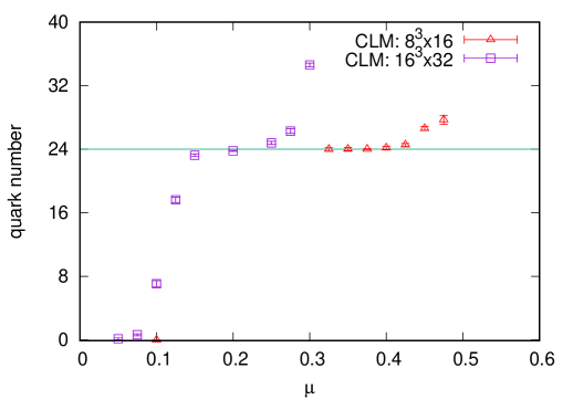
Figure 2: The quark number is plotted against the quark chemical potential $\mu$. The triangles and squares represent the CLM results on $8^{3}\times 16$ and $16^{3}\times 32$ lattices, respectively. We show only the data that are reliable judging from the probability distribution of the drift term.

Surprisingly, for both lattice sizes, we observe a plateau at the height of $N_{\text{q}}=24$, although the plateau region is shifted towards smaller values of $\mu$ for the larger lattice.

Here we provide a physical interpretation of this behavior. The first thing to note is that the spatial size of our lattice is as small as $L_{\text{s}}a\simeq$ 0.36 and 0.73 fm for $L_{\text{s}}=8$ and 16, respectively, since the lattice spacing $a$ is estimated as $a\simeq 0.045$ fm for $\beta=5.7$ and $m=0.01$ with $N_{\mathrm{f}}=4$ staggered fermions. Therefore, the effective gauge coupling is actually small due to the asymptotic freedom, which makes the free fermion picture valid. The energy of a quark is given by $E({\bf p})=\sqrt{{\bf p}^{2}+m^{2}}$ for the discrete momentum ${\bf p}=\frac{2\pi}{L_{\text{s}}}{\bf n}$, where ${\bf n}$ is a three-dimensional integer vector considering the periodic boundary conditions imposed on the spatial directions. At zero temperature and for the quark chemical potential within the region $m\leq\mu\leq\sqrt{(\frac{2\pi}{L_{\text{s}}})^{2}+m^{2}}$, the path integral should be dominated by a state with the maximum number of quarks with zero momentum allowed by the Pauli principle. This number is $4\times 3\times 2=24$, considering the number of flavor, color and spin degrees of freedom. Our results can be qualitatively understood in this way.

In order to have quantitative understanding of our results, we first need to take into account the finite temperature effects considering that the temperature used in our simulation is about $T\simeq$ 270 and 140 MeV for $N_{\text{t}}=$ 16 and 32, respectively. These energy scales are higher than or comparable with the critical temperature $T_{\text{c}}/\sqrt{\sigma}\simeq 0.4$ for $N_{\mathrm{f}}=4$ staggered fermions [21], where $\sigma$ is the string tension. In the forthcoming paper [22], we show that our results can be understood semi-quantitatively by the $\mu$-dependence of the quark number that can be obtained by using the Fermi distribution function for finite temperature. (See Ref. [23] for related work.) Furthermore, the remaining discrepancies can be understood as the effects of the interactions, which is confirmed by calculating the quark number using the lattice perturbation theory.

4 Summary and discussions

In this work we have investigated finite density QCD by the CLM in the low temperature region with reasonably small quark mass using four-flavor staggered fermions on a $16^{3}\times 32$ lattice. In particular, we have found that the quark number exhibits a plateau as a function of the chemical potential. In the plateau region, the quark number turns out to be 24, which is exactly the same as what was found in our previous work on an $8^{3}\times 16$ lattice although the plateau region shifts towards smaller values of $\mu$. We have provided a qualitative understanding of these behaviors based on the free fermion picture at zero temperature. The plateau appears because of the gap in the energy spectrum of fermions due to the finite volume. As the quark chemical potential is increased, only the fermions with zero momentum can be generated. The number 24, which appears as the height of the plateau in the plot of the quark number can be understood as the number of internal degrees of freedom of the fermion. The quark number is expected to jump to the second plateau at $\mu\sim\frac{2\pi}{L_{\text{s}}}$. While this behavior is somewhat obscured by finite temperature effects in our setup, the shift of the plateau region can be understood naturally.

The significance of this result is two-fold. First, the fact that the behaviors observed by the CLM have found a clear physical interpretation confirms further that the method is working and we are getting correct results. While the interpretation shows that we are well within the perturbative regime due to the small spatial extent and the asymptotic freedom, it would be nice to test the method nevertheless in a region in which we can obtain explicit results perturbatively. To our knowledge, the behaviors reported above have never been observed by other methods, which clearly demonstrates the usefulness of the CLM. Second, the condensation of the zero momentum modes may be regarded as the beginning of the formation of the Fermi sphere, which is crucial in color superconductivity. By increasing the lattice size further, the Fermi sphere is expected to grow due to condensation of higher momentum modes. If such behaviors can be observed within the applicability of the CLM, we should be able to study the color superconductivity in the near future.

References

- [1] J. R. Klauder, Phys. Rev. A29, 2036 (1984).
- [2] G. Parisi, Phys. Lett. 131B, 393 (1983).
- [3] G. Aarts, E. Seiler, and I.-O. Stamatescu, Phys. Rev. D81, 054508 (2010), arXiv:0912.3360.
- [4] G. Aarts, F. A. James, E. Seiler, and I.-O. Stamatescu, Eur. Phys. J. C71, 1756 (2011), arXiv:1101.3270.
- [5] J. Nishimura and S. Shimasaki, Phys. Rev. D92, 011501 (2015), arXiv:1504.08359.
- [6] K. Nagata, J. Nishimura, and S. Shimasaki, Phys. Rev. D94, 114515 (2016), arXiv:1606.07627.
- [7] G. Aarts, F. A. James, E. Seiler, and I.-O. Stamatescu, Phys. Lett. B687, 154 (2010), arXiv:0912.0617.
- [8] E. Seiler, D. Sexty, and I.-O. Stamatescu, Phys. Lett. B723, 213 (2013), arXiv:1211.3709.
- [9] Y. Ito and J. Nishimura, JHEP 12, 009 (2016), arXiv:1609.04501.
- [10] F. Attanasio and B. Jager, Eur. Phys. J. C79, 16 (2019), arXiv:1808.04400.
- [11] G. Aarts, L. Bongiovanni, E. Seiler, D. Sexty, and I.-O. Stamatescu, Eur. Phys. J. A49, 89 (2013), arXiv:1303.6425.
- [12] G. Aarts, F. Attanasio, B. Jager, and D. Sexty, JHEP 09, 087 (2016), arXiv:1606.05561.
- [13] D. Sexty, Phys. Lett. B729, 108 (2014), arXiv:1307.7748.
- [14] Z. Fodor, S. D. Katz, D. Sexty, and C. Torok, Phys. Rev. D92, 094516 (2015), arXiv:1508.05260.
- [15] J. B. Kogut and D. K. Sinclair, Phys. Rev. D100, 054512 (2019), arXiv:1903.02622.
- [16] D. K. Sinclair and J. B. Kogut, PoS LATTICE2019, 245 (2019), arXiv:1910.11412.
- [17] K. Nagata, J. Nishimura, and S. Shimasaki, Phys. Rev. D98, 114513 (2018), arXiv:1805.03964.
- [18] Y. Ito et al., PoS LATTICE2018, 146 (2018), arXiv:1811.12688.
- [19] M. Scherzer, Phase transitions in lattice gauge theories:From the numerical sign problem to machine learning., PhD thesis, U. Heidelberg (main), 2019.
- [20] S. Tsutsui et al., JPS Conf. Proc. 26, 024012 (2019).
- [21] J. Engels et al., Phys. Lett. B396, 210 (1997), arXiv:hep-lat/9612018.
- [22] T. Yokota et al., in preparation.
- [23] H. Matsuoka and M. Stone, Phys. Lett. 136B, 204 (1984).