Synchrotron spectra of GRB prompt emission and pulsar wind nebulae

Abstract

Particle acceleration is a fundamental process in many high-energy astrophysical environments and determines the spectral features of their synchrotron emission. We have studied the adiabatic stochastic acceleration (ASA) of electrons arising from the basic dynamics of magnetohydrodynamic (MHD) turbulence and found that the ASA acts to efficiently harden the injected electron energy spectrum. The dominance of the ASA at low energies and the dominance of synchrotron cooling at high energies result in a broken power-law shape of both electron energy spectrum and photon synchrotron spectrum. Furthermore, we have applied the ASA to studying the synchrotron spectra of the prompt emission of gamma-ray bursts (GRBs) and pulsar wind nebulae (PWNe). The good agreement between our theories and observations confirms that the stochastic particle acceleration is indispensable in explaining their synchrotron emission.

1 Introduction

Many cosmic accelerators are huge reservoirs of magnetic energy. The dissipated magnetic energy is converted to energies of particles, accounting for the observed synchrotron emission [1, 2, 3]. In both turbulent and magnetized medium, a proper description of magnetohydrodynamic (MHD) turbulence is crucial for studying the interaction between particles and turbulent magnetic fields and the resulting particle acceleration [4, 5, 6]. Recent theoretical [7, 8] and numerical [9, 10, 11] studies reveal a critical balance between the turbulent motions in the direction perpendicular to the local magnetic field and magnetic wave-like motions parallel to the local magnetic field in MHD turbulence. Accordingly, the turbulent dynamo with magnetic field lines stretched by turbulent motions [12] and the turbulent reconnection of stochastic magnetic fields [8] are also in dynamical balance in MHD turbulence. As a new acceleration mechanism proposed by [13], particles entrained on turbulent magnetic field lines undergo cycles of deceleration in turbulent dynamo regions and acceleration in turbulent reconnection regions, leading to a globally diffusive acceleration process, which we term as “adiabatic stochastic acceleration (ASA)”. The ASA becomes the dominant acceleration process in MHD turbulence when the non-adiabatic resonant scattering of particles by anisotropic MHD turbulence is inefficient [14]. In our recent studies, we applied the ASA to interpreting the Band function spectrum [15] of the prompt emission of gamma-ray bursts (GRBs) [16, 17] and the synchrotron spectra of pulsar wind nebulae (PWNe) [18].

2 Electron energy spectrum resulting from the ASA

The time evolution of the electron energy spectrum $N(E,t)$ is described by

$$\frac{\partial N}{\partial t}=a_{2}\frac{\partial}{\partial E}\Big{(}E\frac{\partial(EN)}{\partial E}\Big{)}+\beta\frac{\partial(E^{2}N)}{\partial E}+Q(E).$$ (1)

The three terms on the RHS correspond to the ASA, radiation losses, and particle injection. The acceleration rate of ASA is

$$a_{2}=\xi\frac{u_{\text{tur}}}{l_{\text{tur}}},$$ (2)

where $l_{\text{tur}}$ and $u_{\text{tur}}$ are the correlation length and speed of turbulence, $\xi=\Delta E/E$ is the cumulative fractional energy change during the trapping of particles within individual turbulent eddies during the eddy turnover time $\tau_{\text{tur}}=l_{\text{tur}}/u_{\text{tur}}$. $\xi$ is of order unity for non-relativistic turbulence and of order $\gamma_{\text{tur}}^{2}$ for relativistic turbulence with $\gamma_{\text{tur}}$ as the turbulence Lorentz factor. In the case of both synchrotron and synchrotron-self-Compton (SSC) losses, $\beta$ is expressed as

$$\beta=\frac{\sigma_{T}cB^{2}(1+Y)}{6\pi(m_{e}c^{2})^{2}},$$ (3)

where $Y$ is the ratio between the powers of SSC and synchrotron radiation and is zero when only synchrotron is considered. Besides, $B$ is the magnetic field strength, $\sigma_{T}$ is the Thomson cross section, $\gamma_{e}$ and $m_{e}$ are the electron Lorentz factor and the electron rest mass, and $c$ is the speed of light. The third term $Q(E)=CE^{-p}$ represents a steady injection of power-law electron spectrum with a power-law index $p$, accounting for other possible instantaneous acceleration processes, e.g., shock acceleration, reconnection acceleration, that generate power-law electron spectra.

In [16, 17], we analytically solved Eq. (1) in the energy range where the ASA dominates over radiation losses. We found that $N(E,t)$ evolves from a spectral shape governed by the injected particle distribution

$$N(E,\tau)=\frac{C^{\prime}\sqrt{\tau}}{\sqrt{\pi}}E^{-p}\exp\Big{(}-\frac{E}{E_{\text{cf}}}\Big{)},$$ (4)

to a hard spectrum under the effect of ASA,

$$N(E,\tau)=\frac{C^{\prime}(E_{u}^{-p+1}-E_{l}^{-p+1})\sqrt{\tau}}{(-p+1)\sqrt{\pi}}E^{-1}\exp\Big{(}-\frac{E}{E_{\text{cf}}}\Big{)},$$ (5)

where $C^{\prime}=C/a_{2}$, $\tau=a_{2}t$, and $E_{l}$ and $E_{u}$ are the lower and upper limits of the energy range of injected electrons. Here $E_{\text{cf}}=a_{2}/\beta$ is the cutoff energy of the ASA, where the acceleration rate equalizes with the cooling rate. This hardening of electron energy spectrum due to the ASA is also illustrated in Fig. 1. It shows that irrespective of the injected spectral form, the ASA leads to diffusive particle acceleration and thus a hard electron energy spectrum with the power-law index approaching $-1$.

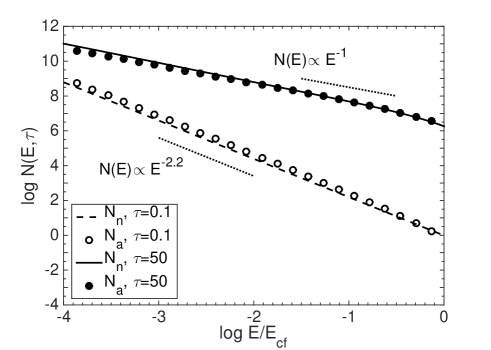
Figure 1: The electron energy spectrum at different times. From [17].

3 Synchrotron spectrum resulting from both ASA and synchrotron cooling

In the energy range $E<E_{\text{cf}}$, the ASA dominates over the synchrotron cooling and leads to the electron energy spectrum as shown in Eq. (5). At higher energies, the synchrotron cooling plays a dominant role in shaping the electron energy spectrum. Depending on the relation between $E_{l}$, $E_{\text{cf}}$, and $E_{c}$, where $E_{c}=1/\beta t$ is the critical cooling energy [19], the electron spectrum and the corresponding synchrotron spectrum exhibit different forms [17], as illustrated in Figs. 2 and 3. The asymptotic functional forms of the flux in different cases are as follows:

Case (i) $E_{l}<E_{\text{cf}}<E_{c}$,

$$F_{\nu}= F_{\nu,\text{max}}\Big{(}\frac{\nu}{\nu_{m}}\Big{)}^{\frac{1}{3}},~{}~{}~{}~{}~{}~{}~{}~{}~{}~{}~{}~{}~{}~{}~{}~{}~{}~{}~{}~{}~{}~{}~{}~{}\nu<\nu_{m},$$ (6a)

$$F_{\nu}= F_{\nu,\text{max}},~{}~{}~{}~{}~{}~{}~{}~{}~{}~{}~{}~{}~{}~{}~{}~{}~{}~{}~{}~{}~{}~{}~{}~{}~{}~{}~{}~{}\nu_{m}<\nu<\nu_{\text{cf}},$$ (6b)

$$F_{\nu}= F_{\nu,\text{max}}\Big{(}\frac{\nu}{\nu_{\text{cf}}}\Big{)}^{-\frac{p-1}{2}},~{}~{}~{}~{}~{}~{}~{}~{}~{}~{}\nu_{\text{cf}}<\nu<\nu_{c},$$ (6c)

$$F_{\nu}= F_{\nu,\text{max}}\Big{(}\frac{\nu_{c}}{\nu_{\text{cf}}}\Big{)}^{-\frac{p-1}{2}}\Big{(}\frac{\nu}{\nu_{c}}\Big{)}^{-\frac{p}{2}},~{}~{}~{}~{}~{}~{}\nu_{c}<\nu.$$ (6d)

Case (ii) $E_{l}<E_{c}<E_{\text{cf}}$,

$$F_{\nu}= F_{\nu,\text{max}}\Big{(}\frac{\nu}{\nu_{m}}\Big{)}^{\frac{1}{3}},~{}~{}~{}~{}~{}~{}~{}~{}~{}~{}~{}~{}~{}~{}~{}~{}~{}~{}~{}~{}~{}~{}~{}~{}\nu<\nu_{m},$$ (7a)

$$F_{\nu}= F_{\nu,\text{max}},~{}~{}~{}~{}~{}~{}~{}~{}~{}~{}~{}~{}~{}~{}~{}~{}~{}~{}~{}~{}~{}~{}~{}~{}~{}~{}~{}~{}\nu_{m}<\nu<\nu_{\text{cf}},$$ (7b)

$$F_{\nu}= F_{\nu,\text{max}}\Big{(}\frac{\nu}{\nu_{\text{cf}}}\Big{)}^{-\frac{p}{2}},~{}~{}~{}~{}~{}~{}~{}~{}~{}~{}~{}~{}~{}~{}~{}~{}~{}~{}~{}~{}~{}~{}\nu_{\text{cf}}<\nu.$$ (7c)

Case (iii) $E_{c}<E_{\text{cf}}<E_{l}$,

$$F_{\nu}= F_{\nu,\text{max}}\Big{(}\frac{\nu}{\nu_{m}}\Big{)}^{\frac{1}{3}},~{}~{}~{}~{}~{}~{}~{}~{}~{}~{}~{}~{}~{}~{}~{}~{}~{}~{}~{}~{}~{}~{}~{}~{}\nu<\nu_{m},$$ (8a)

$$F_{\nu}= F_{\nu,\text{max}},~{}~{}~{}~{}~{}~{}~{}~{}~{}~{}~{}~{}~{}~{}~{}~{}~{}~{}~{}~{}~{}~{}~{}~{}~{}~{}~{}~{}\nu_{m}<\nu<\nu_{\text{cf}},$$ (8b)

$$F_{\nu}= F_{\nu,\text{max}}\Big{(}\frac{\nu}{\nu_{\text{cf}}}\Big{)}^{-\frac{1}{2}},~{}~{}~{}~{}~{}~{}~{}~{}~{}~{}~{}~{}~{}~{}\nu_{\text{cf}}<\nu<\nu_{l},$$ (8c)

$$F_{\nu}= F_{\nu,\text{max}}\Big{(}\frac{\nu_{l}}{\nu_{\text{cf}}}\Big{)}^{-\frac{1}{2}}\Big{(}\frac{\nu}{\nu_{l}}\Big{)}^{-\frac{p}{2}},~{}~{}~{}~{}~{}~{}~{}~{}~{}~{}\nu_{l}<\nu.$$ (8d)

Case (iv) $E_{c}<E_{l}<E_{\text{cf}}$,

$$F_{\nu}= F_{\nu,\text{max}}\Big{(}\frac{\nu}{\nu_{m}}\Big{)}^{\frac{1}{3}},~{}~{}~{}~{}~{}~{}~{}~{}~{}~{}~{}~{}~{}~{}~{}~{}~{}~{}~{}~{}~{}~{}~{}~{}\nu<\nu_{m},$$ (9a)

$$F_{\nu}= F_{\nu,\text{max}},~{}~{}~{}~{}~{}~{}~{}~{}~{}~{}~{}~{}~{}~{}~{}~{}~{}~{}~{}~{}~{}~{}~{}~{}~{}~{}~{}~{}\nu_{m}<\nu<\nu_{\text{cf}},$$ (9b)

$$F_{\nu}= F_{\nu,\text{max}}\Big{(}\frac{\nu}{\nu_{\text{cf}}}\Big{)}^{-\frac{p}{2}},~{}~{}~{}~{}~{}~{}~{}~{}~{}~{}~{}~{}~{}~{}~{}~{}~{}~{}~{}~{}~{}~{}~{}\nu_{\text{cf}}<\nu.$$ (9c)

We note that the low-frequency tail $F_{\nu}\propto\nu^{1/3}$ comes from the synchrotron single-particle emission spectrum [20, 21].

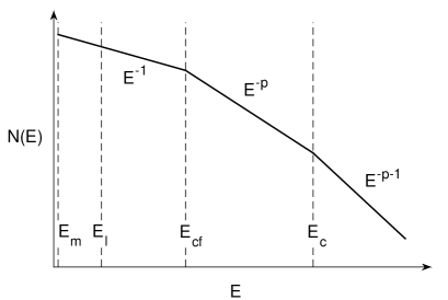
(a) Case (i)

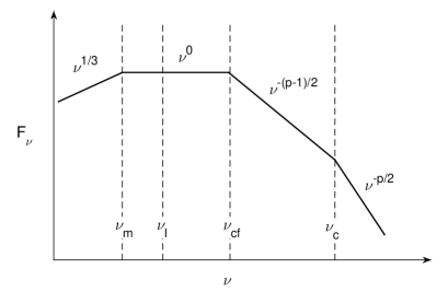
(b) Case (i)

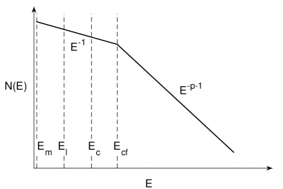
(c) Case (ii)

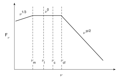
(d) Case (ii)

Figure 2: The electron energy spectrum ((a) and (c)) and the corresponding synchrotron spectrum ((b) and (d)) in Case (i) and in Case (ii). From [17].

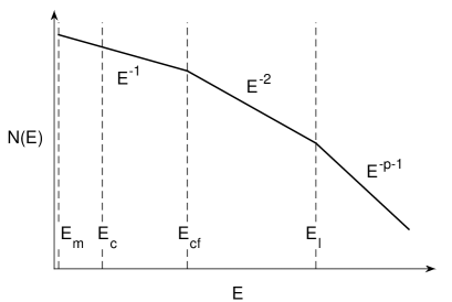
(a) Case (iii)

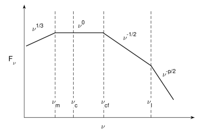
(b) Case (iii)

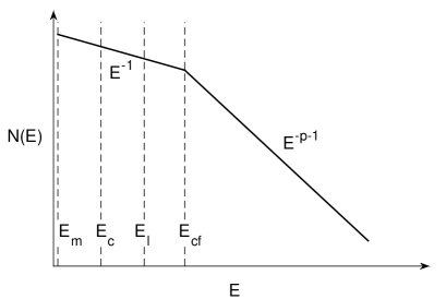
(c) Case (iv)

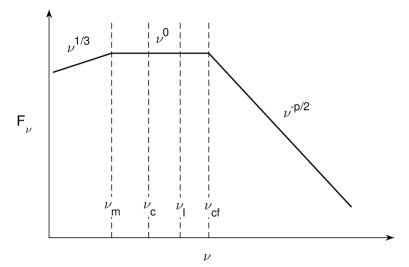
(d) Case (iv)

Figure 3: The electron energy spectrum ((a) and (c)) and the corresponding synchrotron spectrum ((b) and (d)) in Case (iii) and in Case (iv). From [17].

4 Application to the synchrotron spectra of GRB prompt emission

The ASA can generally take place in MHD turbulence and dominate over other stochastic acceleration mechanisms, e.g., gyroresonance, when the pitch-angle scattering is inefficient. Therefore, we have explored the application of the ASA to the stochastic acceleration process in different astrophysical environments, which are both magnetized and turbulent. In this section and §5, we will discuss the ASA in the context of GRBs and PWNe as examples.

The empirical Band spectrum [15] is usually used to describe the time-averaged synchrotron spectrum of GRB prompt emission. It is characterized by a low-energy spectral index $\alpha_{s}$, a break energy $E_{b}$, and a high-energy spectral index $\beta_{s}$. The distributions of $\alpha_{s}$ and $\beta_{s}$ are centered around $-1$ and $-2.25$, respectively, and $E_{b}$ is on the order of $100$ keV [22]. The above spectral features, especially the hard low-energy spectrum, cannot be well explained by either the thermal model [23, 24] or the synchrotron model [25, 21, 26] of GRBs.

In [16, 17], we investigated the ASA in the magnetized and turbulent GRB outflow [1, 2] and found that it can naturally account for the hard low-energy spectrum of GRB prompt emission. The synchrotron spectrum in both Case (ii) and Case (iv) (§3) agrees with the Band spectrum. As a result of the ASA, there is $N(\nu)\propto F_{\nu}/\nu\propto\nu^{-1}$ in the frequency range $(\nu_{m},\nu_{\text{cf}})$. The high-energy synchrotron spectrum is related to the injected electron distribution, and $\beta_{s}=-2.25$ corresponds to $p=2.5$, which can be explained by other first-order Fermi acceleration processes, such as the shock acceleration and the reconnection acceleration [27]. $E_{b}$ is related to $E_{\text{cf}}$. The photon energy corresponding to $E_{\text{cf}}$ in the observer frame is [17],

$$E_{s,\text{cf,obs}}\simeq 385\text{keV}~{}\Big{(}\frac{1+z}{2}\Big{)}^{-1}\Gamma_{2}^{-0.2}L_{52}^{0.6}r_{15}^{-1.2},$$ (10)

where $z$ is the redshift, $\Gamma=100\Gamma_{2}$ is the bulk Lorentz factor, $L=10^{52}$ erg s${}^{-1}L_{52}$ is the total isotropic luminosity, and $r=10^{15}$ cm$r_{15}$ is the radius of the emission region [1]. It has the same order of magnitude as $E_{b}$ that is indicated by observations.

5 Application to the synchrotron spectra of PWNe

In [18], we applied the ASA to explaining the synchrotron spectra of magnetized and turbulent PWNe and found a good agreement between the analytical spectral shapes (§3) and the observed broad-band synchrotron spectra of different PWNe (see Figs. 4 and 5). Moreover, the observed spectral break is related to $E_{\text{cf}}$ and can be used to constrain the acceleration timescale of the ASA $\tau_{\text{acc}}=1/a_{2}$. If the synchrotron spectrum of a PWN falls in Case (ii) or Case (iv), there is

$$\Big{(}\frac{\tau_{\text{acc}}}{1~{}\text{kyr}}\Big{)}\Big{(}\frac{B}{100~{}\mu\text{G}}\Big{)}^{\frac{3}{2}}=26.5\Big{(}\frac{\Gamma}{1}\Big{)}^{\frac{1}{2}}\Big{(}\frac{E_{\text{ph,b}}}{10^{-2}~{}\text{eV}}\Big{)}^{-\frac{1}{2}},$$ (11)

where $B$ is the magnetic field strength in the PWN, $\Gamma$ is the bulk Lorentz factor of the mildly relativistic flow in the PWN, and $E_{\text{ph,b}}$ is the observed energy break of synchrotron spectrum. If the synchrotron spectrum of a PWN falls in Case (i) or Case (iii), there is

$$\Big{(}\frac{\tau_{\text{acc}}}{1~{}\text{kyr}}\Big{)}\Big{(}\frac{B}{100~{}\mu\text{G}}\Big{)}^{\frac{3}{2}}=837.0\Big{(}\frac{\Gamma}{1}\Big{)}^{\frac{1}{2}}\Big{(}\frac{E_{\text{ph,b1}}}{10^{-5}~{}\text{eV}}\Big{)}^{-\frac{1}{2}},$$ (12)

where $E_{\text{ph,b1}}$ is the observed energy break at a lower energy (see Fig. 4). In the case when the spectral shape in the infrared band cannot be well determined, we have

$$26.5\Big{(}\frac{\Gamma}{1}\Big{)}^{\frac{1}{2}}\Big{(}\frac{E_{\text{ph,b}}}{10^{-2}~{}\text{eV}}\Big{)}^{-\frac{1}{2}}\leq\Big{(}\frac{\tau_{\text{acc}}}{1~{}\text{kyr}}\Big{)}\Big{(}\frac{B}{100~{}\mu\text{G}}\Big{)}^{\frac{3}{2}}\leq 837.0\Big{(}\frac{\Gamma}{1}\Big{)}^{\frac{1}{2}}\Big{(}\frac{E_{\text{ph,b1}}}{10^{-5}~{}\text{eV}}\Big{)}^{-\frac{1}{2}},$$ (13)

as illustrated in Fig. 6.

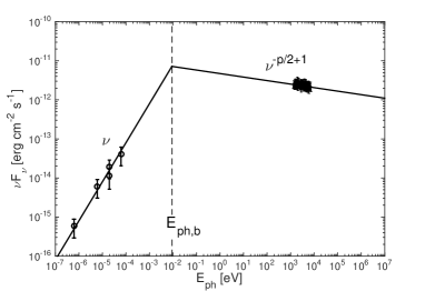
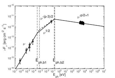
Figure 4: Comparison between analytical spectral shapes and observational data for the Mouse PWN. Circles, square, and dots represent radio, infrared, and X-ray data, respectively. See the original figure and references in [18].

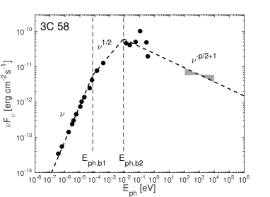
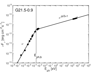
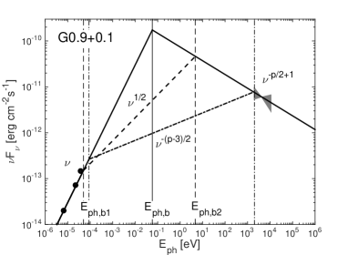
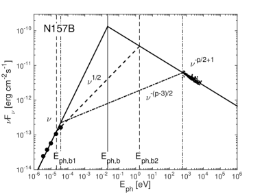
Figure 5: Comparison between analytical spectral shapes and observational data for different PWNe. See the original figures and references in [18].

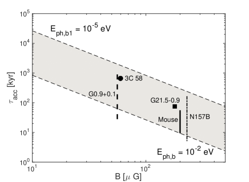
Figure 6: $\tau_{\text{acc}}$ vs. $B_{\text{eq}}$ of the PWNe, where $B_{\text{eq}}$ is the magnetic field strength under the assumption of equipartition between particle and magnetic energies. The shaded region is bounded by Eq. (13). From [18].

6 Summary

As a new stochastic acceleration mechanism, the ASA arises from the basic dynamics of MHD turbulence involving both turbulent dynamo and turbulent reconnection of magnetic fields. Different from other stochastic acceleration mechanisms, it is highly efficient as particles undergo the first-order Fermi process within individual turbulent eddies. It is also not subject to the turbulence anisotropy effect, which makes the gyroresonance with Alfvénic turbulence inefficient.

The ASA naturally hardens the injected electron spectrum and results in a hard electron spectrum in the energy range dominated by the ASA. Under the effects of both ASA and radiation cooling, the electron spectrum exhibits a broken power-law shape. The resulting synchrotron spectrum well explains the synchrotron spectrum of GRB prompt emission, as well as the broad-band synchrotron spectrum of a PWN.

The ASA is a general acceleration mechanism in MHD turbulence. Besides GRBs and PWNe, the application of the ASA to other high-energy astrophysical environments, e.g., radio galaxies, blazars, will be investigated in our future work.

References

- [1] Zhang B and Yan H 2011 ApJ 726 90 (Preprint 1011.1197)
- [2] Deng W, Li H, Zhang B and Li S 2015 ApJ 805 163 (Preprint 1501.07595)
- [3] Lazarian A, Zhang B and Xu S 2018 arXiv: 1801.04061 (Preprint 1801.04061)
- [4] Xu S and Yan H 2013 ApJ 779 140 (Preprint 1307.1346)
- [5] Xu S, Yan H and Lazarian A 2016 ApJ 826 166 (Preprint 1506.05585)
- [6] Xu S and Lazarian A 2018 ApJ 868 36 (Preprint 1810.07726)
- [7] Goldreich P and Sridhar S 1995 ApJ 438 763–775
- [8] Lazarian A and Vishniac E T 1999 ApJ 517 700–718 (Preprint arXiv:astro-ph/9811037)
- [9] Cho J and Vishniac E T 2000 ApJ 539 273–282 (Preprint arXiv:astro-ph/0003403)
- [10] Maron J and Goldreich P 2001 ApJ 554 1175–1196 (Preprint arXiv:astro-ph/0012491)
- [11] Cho J, Lazarian A and Vishniac E T 2002 ApJ 564 291–301 (Preprint arXiv:astro-ph/0105235)
- [12] Xu S and Lazarian A 2016 ApJ 833 215 (Preprint 1608.05161)
- [13] Brunetti G and Lazarian A 2016 MNRAS 458 2584–2595 (Preprint 1603.00458)
- [14] Yan H and Lazarian A 2002 Physical Review Letters 89 B1102+ (Preprint arXiv:astro-ph/0205285)
- [15] Band D, Matteson J, Ford L, Schaefer B, Palmer D, Teegarden B, Cline T, Briggs M, Paciesas W, Pendleton G, Fishman G, Kouveliotou C, Meegan C, Wilson R and Lestrade P 1993 ApJ 413 281–292
- [16] Xu S and Zhang B 2017 ApJL 846 L28 (Preprint 1708.08029)
- [17] Xu S, Yang Y P and Zhang B 2018 ApJ 853 43 (Preprint 1711.03943)
- [18] Xu S, Klingler N, Kargaltsev O and Zhang B 2019 ApJ 872 10 (Preprint 1812.10827)
- [19] Sari R, Piran T and Narayan R 1998 ApJL 497 L17–L20 (Preprint astro-ph/9712005)
- [20] Meszaros P and Rees M J 1993 ApJL 418 L59 (Preprint astro-ph/9309011)
- [21] Katz J I 1994 ApJL 432 L107–L109 (Preprint astro-ph/9312034)
- [22] Preece R D, Briggs M S, Mallozzi R S, Pendleton G N, Paciesas W S and Band D L 2000 ApJS 126 19–36 (Preprint astro-ph/9908119)
- [23] Beloborodov A M 2010 MNRAS 407 1033–1047 (Preprint 0907.0732)
- [24] Deng W and Zhang B 2014 ApJ 785 112 (Preprint 1402.5364)
- [25] Rees M J and Meszaros P 1992 MNRAS 258 41P–43P
- [26] Tavani M 1996 ApJ 466 768
- [27] de Gouveia dal Pino E M and Lazarian A 2005 A&A 441 845–853