On the broad-band synchrotron spectra of pulsar wind nebulae

Abstract

As shown by broad-band observations, pulsar wind nebulae (PWNe) are characterized by a broken power-law spectrum of synchrotron emission. Based on the modern magnetohydrodynamic (MHD) turbulence theories, we investigate the re-acceleration of electrons in the PWN through the adiabatic stochastic acceleration (ASA), which arises from fundamental dynamics of MHD turbulence. The ASA acts to flatten the injected energy spectrum of electrons at low energies, while synchrotron cooling results in a steep spectrum of electrons at high energies. Their dominance in different energy ranges leads to a flat radio spectrum ($F_{\nu}$) and a steep X-ray spectrum. Our analytical spectral shapes generally agree well with the observed synchrotron spectra of radio- and X-ray-bright PWNe. The spectral break corresponding to the balance between the ASA and synchrotron losses provides a constraint on the acceleration timescale of the ASA and the magnetic field strength in the PWN.

1. Introduction

Poynting-flux-dominated pulsar winds (PWs) and their surrounding pulsar wind nebulae (PWNe) serve as a representative example for studying the mechanisms of energy dissipation and particle acceleration in high-energy astrophysical environments. Broad-band observations reveal a broken power law consisting of a flat radio spectrum ($F_{\nu}$) and a steeper X-ray spectrum as a characteristic radiation spectrum of PWNe (e.g.,Chevalier 2005; Gaensler & Slane 2006; Reynolds et al. 2017). Although the multi-wavelength radiation is believed to be synchrotron in radio and X-rays, the broad-band spectral shape is not well understood.

The stochastic nature of turbulent magnetic fields is frequently invoked to model the flat spectrum $F_{\nu}$ of radio emission (e.g., Fleishman & Bietenholz 2007; Tanaka & Asano 2017). Turbulent magnetic fields in PWNe are naturally expected and also indicated by observations (Reynolds & Aller, 1988; Yusef-Zadeh & Gaensler, 2005; Moran et al., 2013; Ma et al., 2016) and simulations (Porth et al., 2014b). Magnetohydrodynamic (MHD) turbulence is a highly nonlinear problem. Recent theoretical studies (Goldreich & Sridhar 1995; Lazarian & Vishniac 1999, hereafter LV99) offer new insights into its nonlinear dynamics. This nonlinear character cannot be captured by a superposition of linear waves, which was traditionally assumed for modeling MHD turbulence (Giacalone & Jokipii, 1999). The updated understanding of fundamental properties of MHD turbulence brings paradigm changes in studying important physical processes, e.g., magnetic reconnection and dissipation (LV99; Zhang & Yan 2011; Deng et al. 2015; Lazarian et al. 2018), particle acceleration and radiation (Pohl et al., 2005; Yan et al., 2008; Brunetti & Lazarian, 2007; Guo et al., 2017; Xu et al., 2016; Xu & Zhang, 2017; Xu et al., 2018; Xu & Lazarian, 2018), related to high-energy astrophysical phenomena.

Alfvén modes dominate the dynamics of MHD turbulence and carry the majority of turbulent kinetic energy (Cho & Lazarian, 2003). The anisotropic scaling of Alfvénic turbulence in the frame of the local magnetic field (LV99) is a direct consequence of its nonlinear dynamics. Due to the turbulence anisotropy, the stochastic particle acceleration via gyroresonance with Alfvénic turbulence is inefficient (Chandran, 2000; Yan & Lazarian, 2002). For relativistic particles that undergo inefficient gyroresonance scattering, a new acceleration mechanism arising from the basic dynamics of Alfvénic turbulence is applicable (Brunetti & Lazarian, 2016). The stochastic dynamo stretching and reconnection shrinking of turbulent magnetic fields lead to a globally diffusive acceleration of particles entrained on field lines. Systematic energy change of particles during the trapping in individual turbulent eddies makes the acceleration highly efficient. Xu & Zhang (2017); Xu et al. (2018) term it as “adiabatic stochastic acceleration (ASA)” to distinguish it from the non-adiabatic stochastic acceleration through gyroresonance scattering and apply it to interpreting the Band function spectrum commonly observed in gamma-ray bursts (GRBs) (Band et al., 1993; Preece et al., 2000). The ASA- and synchrotron cooling-dominated electron energy distributions explain well the hard low-energy spectrum and softer high-energy spectrum of GRB prompt emission, respectively. As the ASA is generally applicable to particle acceleration in turbulent magnetic fields, here we introduce the ASA and examine its effect, together with synchrotron cooling, on shaping the broad-band synchrotron spectra of PWNe. We also consider the turbulent reconnection of magnetic fields in PWs to account for the source of turbulence, as well as the injection of energetic particles for further ASA and synchrotron radiation in PWNe.

Based on the modern understanding of MHD turbulence and its interaction with energetic particles mentioned above, we apply our analytical model for describing the ASA and radiation loss to PWNe and aim at providing a general explanation for their broken power-law spectra. The structure of this paper is as follows. In Section 2, we present our analytical model and elucidate the physical origin of the broken power-law spectrum in the context of a PWN. In Section 3, we take the Mouse PWN and some other PWNe as examples for applying our theoretical model to the observed broad-band synchrotron spectra. Lastly, a discussion and a summary are given in Section 4 and Section 5, respectively.

2. Physical origin of a broken power-law spectrum of a PWN

2.1. Turbulent reconnection in the PW

To facilitate the transition from the Poynting flux-dominated (i.e., high-$\sigma$) pulsar wind (Arons, 2002) to the particle energy flux-dominated (i.e., low-$\sigma$) downstream of the termination shock (Rees & Gunn, 1974; Kennel & Coroniti, 1984; Begelman & Li, 1992; Bogovalov et al., 2005), efficient dissipative processes are necessary to convert the magnetic energy to kinetic energy in the upstream wind or at the termination shock. Magnetic reconnection serves as the required dissipation mechanism (Del Zanna et al., 2016). It can occur in the striped wind with alternating magnetic fields (Coroniti, 1990; Lyubarsky & Kirk, 2001), as well as the kink-unstable polar jet (Begelman, 1998; Pavlov et al., 2003; Mizuno et al., 2011; Mignone et al., 2013).

In resistive MHD theory, the magnetic reconnection depends on the slow resistive diffusion of magnetic fields (Sweet, 1958; Parker, 1957). In the presence of turbulence, turbulent velocities dominate the magnetic field dynamics in the direction perpendicular to the local magnetic field (LV99). The turbulent velocities act to increase the magnetic field gradients along the turbulent energy cascade toward smaller scales, and thus enhance the reconnection and determine the actual reconnection efficiency. In strongly magnetized turbulence, the reconnection rate is given by (LV99)

$$v_{\text{rec}}\approx V_{A}\sqrt{\frac{L_{i}}{L_{x}}}M_{A}^{2},$$ (1)

when the injection scale of turbulence $L_{i}$ is smaller than the length of the current sheet $L_{x}$, and

$$v_{\text{rec}}\approx V_{A}\sqrt{\frac{L_{x}}{L_{i}}}M_{A}^{2}$$ (2)

when $L_{i}>L_{x}$. Here $v_{\text{rec}}$ is the reconnection speed, $V_{A}$ is the Alfvén speed, and $M_{A}$ is the ratio of the turbulent speed at $L_{i}$ to $V_{A}$. Without the constraint imposed by microscopic diffusion process, turbulent reconnection can be highly efficient with $v_{\text{rec}}$ up to $V_{A}$. Numerical experiments in both non-relativistic (Kowal et al., 2009) and relativistic (Takamoto et al., 2015; East et al., 2015; Zrake & East, 2016) plasmas confirm that the turbulent reconnection is universal with respect to microscopic physics, e.g., resistive diffusion.

Magnetic reconnection itself acts as a source of turbulence. The magnetostatic free energy carried by the striped wind can be readily converted to turbulent energy via magnetic reconnection (East et al., 2015; Zrake & East, 2016). The generated turbulence in turn boosts the reconnection efficiency as discussed above (Kowal et al., 2017). This positive feedback can result in a runaway reconnection and explosive release of magnetic energy, accounting for the energy source of observed $\gamma$-ray flares from e.g. the Crab Nebula (Tavani et al., 2011; Abdo et al., 2011). The development of both turbulence and turbulent reconnection of magnetic fields have been observed in numerical simulations of the pulsar striped wind, e.g., Zrake (2016).

Moreover, magnetic reconnection can also efficiently energize particles (de Gouveia dal Pino & Lazarian, 2005; Kowal et al., 2011, 2012; del Valle et al., 2016), which supplies the PWN with a power-law population of energetic electrons. By adopting a simple treatment analogous to that for the first-order Fermi acceleration at shocks, de Gouveia dal Pino & Lazarian (2005) derived a power-law index $2.5$ for the reconnection-accelerated particles. Beyond the termination shock, the spectrum of the accelerated electrons injected into the PWN will be affected by both the ASA and synchrotron cooling in the turbulent magnetic fields downstream.

2.2. ASA in the PWN

Due to the magnetic reconnection in the striped wind, the PWN is expected to be fully turbulent. The Kolmogorov-like magnetic energy spectrum has been found in 3D relativistic MHD simulations of PWNe, e.g., Porth et al. (2014b), which is a typical spectral form of turbulent magnetic fields in strong MHD turbulence (Maron & Goldreich, 2001; Cho & Lazarian, 2003).

In strong MHD turbulence with increased turbulence anisotropy toward smaller scales, the turbulent eddies at the resonant scale of gyroresonance are highly elongated along the magnetic field. With the perpendicular scale of the turbulent eddies much smaller than the parallel resonant scale, particles interact with many uncorrelated turbulent eddies within one gyro orbit, and thus the gyroresonance scattering is inefficient (Chandran, 2000; Yan & Lazarian, 2002). In the absence of efficient scattering, relativistic particles can slide along magnetic field lines. Obviously, the magnetic field variation is slow with respect to the motion of particles. Within the traps of turbulent eddies, the second (longitudinal) adiabatic invariant of the particles bouncing between the “mirror points” applies. As there are statistically distributed reconnection and dynamo regions in strong MHD turbulence (Xu & Lazarian, 2016), after cycles of acceleration in turbulent reconnection regions with shrinking field lines and cycles of deceleration in turbulent dynamo regions with stretched field lines, the particles have a diffusive energy gain (Brunetti & Lazarian, 2016). We term this acceleration process as the “adiabatic stochastic acceleration (ASA)” (Xu & Zhang, 2017; Xu et al., 2018).

The acceleration rate of the ASA is

$$a_{A}=\xi\frac{u_{\text{tur}}}{l_{\text{tur}}},$$ (3)

where $l_{\text{tur}}$ is the characteristic scale of turbulent magnetic fields, $u_{\text{tur}}$ is the turbulent speed at $l_{\text{tur}}$, and their ratio gives the corresponding turbulent eddy-turnover time $\tau_{\text{tur}}$. $\xi$ represents the cumulative fractional energy change during $\tau_{\text{tur}}$. As relativistic particles undergo the first-order Fermi process within individual eddies, given the number of bounces $\sim c/u_{\text{tur}}$ and the energy change per bounce $\sim u_{\text{tur}}/c$, where $c$ is the speed of light, we can easily see that $\xi$ is of order unity. Thus the ASA is a very efficient stochastic acceleration mechanism compared to the second-order Fermi acceleration associated with gyroresonance scattering.

2.3. Synchrotron spectrum under the effects of ASA and synchrotron cooling

The stochastic acceleration generally leads to energy diffusion and a hard energy spectrum of particles. We consider a steady injection of a power-law distribution of electrons originating from the magnetic reconnection sites in the PW (Section 2.1),

$$Q(E)=CE^{-p},~{}~{}E_{l}<E<E_{u}.$$ (4)

At a given reference energy, $C$ is the electron number per unit energy per unit time, $p$ is the power-law index, and $E_{l}$ and $E_{u}$ are the lower and upper energy limits, respectively. Due to the ASA, the energy distribution of electrons spreads out in energy space following (Melrose, 1969)

$$E\sim\exp(\pm 2\sqrt{a_{A}t}).$$ (5)

The injected energy spectrum evolves with time $t$ and approaches a universal form (Xu et al., 2018)

$$N(E,t)=\frac{C(E_{u}^{-p+1}-E_{l}^{-p+1})\sqrt{t}}{(-p+1)\sqrt{\pi a_{A}}}E^{-1}\exp\Big{(}-\frac{E}{E_{\text{cf}}}\Big{)},$$ (6)

$$~{}~{}~{}~{}~{}~{}~{}~{}~{}~{}~{}~{}~{}~{}~{}~{}~{}~{}~{}~{}~{}~{}~{}~{}~{}~{}~{}~{}~{}~{}~{}~{}~{}~{}~{}~{}~{}~{}~{}~{}~{}~{}~{}~{}~{}~{}~{}~{}~{}~{}~{}~{}~{}~{}~{}~{}~{}~{}~{}~{}~{}~{}~{}~{}E_{m}<E<E_{\text{cf}}.$$

The resulting energy spectrum has a minimum energy $E_{m}$. It is smaller than $E_{l}$ as the energy spectrum under the effect of ASA tends to have a larger energy spread than that of the injected electrons (Eq. (5)). $E_{\text{cf}}$ is the cutoff energy of the ASA and has the expression

$$E_{\text{cf}}=\frac{a_{A}}{\beta},$$ (7)

corresponding to the equalization between $a_{A}$ and synchrotron cooling rate. Here the parameter $\beta$ is given by

$$\beta=\frac{P_{\text{syn}}}{E^{2}}=\frac{\sigma_{T}cB^{2}}{6\pi(m_{e}c^{2})^{2}},$$ (8)

where $P_{\text{syn}}$ is the power of synchrotron radiation, $B$ is the magnetic field strength, $\sigma_{T}$ is the Thomson cross section, and $m_{e}$ is the electron rest mass. Different from a steep energy spectrum of electrons, for which the minimum energy is the characteristic electron energy, for a hard electron spectrum in Eq. (6), the upper cutoff energy $E_{\text{cf}}$ dominates the integral,

$$\int_{E_{m}}^{E_{\text{cf}}}EN(E)dE\approx\frac{C(E_{u}^{-p+1}-E_{l}^{-p+1})\sqrt{t}}{(-p+1)\sqrt{\pi a_{A}}}E_{\text{cf}}=\epsilon\dot{E}t,$$ (9)

where we assume $E_{u}<E_{\text{cf}}$ and $E_{m}\ll E_{\text{cf}}$, $\dot{E}$ is the spin-down power of the pulsar, and $\epsilon$ is the fraction of the spin-down energy converted to the particle energy. To confront the above relation to observations, a detailed modeling of the particle acceleration in the PW is needed, which is beyond the scope of the current paper.

We next consider that the injected electrons have sufficiently high energies with $E_{\text{cf}}<E_{u}$. The hard electron energy distribution below $E_{\text{cf}}$ is attributed to the ASA, while the distribution at energies above $E_{\text{cf}}$ is governed by synchrotron cooling effect. By defining the critical cooling energy (Sari et al., 1998)

$$E_{c}=P_{\text{syn}}t=\frac{1}{\beta t},$$ (10)

we see that the injected electrons with $E>E_{c}>E_{\text{cf}}$ cool down to $E_{c}$ within time t. But the electrons with $E<E_{\text{cf}}$ do not cool because of the ASA, irrespective of the value of $E_{c}$. It means that the overall system is always in slow cooling regime.

Given $E_{m}$ and $E_{u}$ as the lower and upper energy limits of the entire electron energy spectrum, depending on the relation between $E_{l}$, $E_{\text{cf}}$, and $E_{c}$, the electron spectrum at $E>E_{\text{cf}}$ can exhibit different forms (Xu et al., 2018).

Case (i): $E_{c}<E_{l}<E_{\text{cf}}$

In the energy range above $E_{\text{cf}}$, the cooled electrons follow a steep spectrum (Kardashev, 1962)

$$N(E)=\frac{CE^{-(p+1)}}{\beta(p-1)}.$$ (11)

Combining Eqs. (6) and (11), we illustrate the asymptotic behavior of the electron spectrum over a broad energy range in Fig. 1(a). The corresponding synchrotron spectrum is

$$\nu F_{\nu}= \nu F_{\nu,\text{max}}\propto\nu,~{}~{}~{}~{}~{}~{}~{}~{}~{}~{}~{}~{}~{}~{}~{}~{}~{}~{}~{}~{}~{}~{}~{}~{}~{}~{}~{}~{}\nu<\nu_{\text{cf}},$$ (12a)

$$\nu F_{\nu}= \nu F_{\nu,\text{max}}\Big{(}\frac{\nu}{\nu_{\text{cf}}}\Big{)}^{-\frac{p}{2}}\propto\nu^{-\frac{p}{2}+1},~{}~{}~{}\nu>\nu_{\text{cf}},$$ (12b)

as displayed in Fig. 1(b), where $\nu_{\text{cf}}$ is the frequency related to $E_{\text{cf}}$, $F_{\nu}$ is the flux density at frequency $\nu$, and $F_{\nu,\text{max}}$ is the maximum value of $F_{\nu}$.

Case (ii): $E_{c}<E_{\text{cf}}<E_{l}$

In the energy range above $E_{l}$, the same steep electron spectrum as in Eq. (11) applies. Moreover, driven by the cooling effect, the injected electron energy distribution extends down to lower energies. In the energy range $E_{\text{cf}}<E<E_{l}$, the electron spectrum is $N(E)\sim E^{-2}$, with the injection and radiation losses of electrons in equilibrium (Melrose, 1969). Accordingly, the entire electron spectrum contains three segments, as shown in Fig. 1(c). The corresponding synchrotron spectrum is (see Fig. 1(d)),

$$\nu F_{\nu}= \nu F_{\nu,\text{max}}\propto\nu,~{}~{}~{}~{}~{}~{}~{}~{}~{}~{}~{}~{}~{}~{}~{}~{}~{}~{}~{}~{}~{}~{}~{}~{}~{}~{}~{}~{}~{}~{}\nu<\nu_{\text{cf}},$$ (13a)

$$\nu F_{\nu}= \nu F_{\nu,\text{max}}\Big{(}\frac{\nu}{\nu_{\text{cf}}}\Big{)}^{-\frac{1}{2}}\propto\nu^{\frac{1}{2}},~{}~{}~{}\nu_{\text{cf}}<\nu<\nu_{l},$$ (13b)

$$\nu F_{\nu}= \nu F_{\nu,\text{max}}\Big{(}\frac{\nu_{l}}{\nu_{\text{cf}}}\Big{)}^{-\frac{1}{2}}\Big{(}\frac{\nu}{\nu_{l}}\Big{)}^{-\frac{p}{2}}\propto\nu^{-\frac{p}{2}+1},$$

$$\nu F_{\nu}= ~{}~{}~{}~{}~{}~{}~{}~{}~{}~{}~{}~{}~{}~{}~{}~{}~{}~{}~{}~{}~{}~{}~{}~{}~{}~{}~{}~{}~{}~{}~{}~{}~{}~{}~{}~{}~{}~{}~{}~{}~{}~{}~{}~{}~{}~{}~{}~{}~{}~{}~{}~{}\nu>\nu_{l},$$ (13c)

where $\nu_{l}$ is related to $E_{l}$.

Case (iii): $E_{l}<E_{c}<E_{\text{cf}}$

As shown in Fig. 2(a), $N(E)$ in this situation has the same form as that in Case (i). The resulting synchrotron spectrum also has the same shape as that in Eq. (12b), which can be seen in Fig. 2(b).

Case (iv): $E_{l}<E_{\text{cf}}<E_{c}$

The cooled electrons at $E>E_{c}$ still follow the spectral shape as in Eq. (11), while the electrons in the energy range $E_{\text{cf}}<E<E_{c}$ are not subjected to the cooling effect, so their original spectral form remains (see Fig. 2(c)). Then the synchrotron spectrum is given by (Fig. 1(d)),

$$\nu F_{\nu}= \nu F_{\nu,\text{max}}\propto\nu,~{}~{}~{}~{}~{}~{}~{}~{}~{}~{}~{}~{}~{}~{}~{}~{}~{}~{}~{}~{}~{}~{}~{}~{}~{}~{}~{}~{}~{}~{}\nu<\nu_{\text{cf}},$$ (14a)

$$\nu F_{\nu}= \nu F_{\nu,\text{max}}\Big{(}\frac{\nu}{\nu_{\text{cf}}}\Big{)}^{-\frac{p-1}{2}}\propto\nu^{-\frac{p-3}{2}},$$

$$\nu F_{\nu}= ~{}~{}~{}~{}~{}~{}~{}~{}~{}~{}~{}~{}~{}~{}~{}~{}~{}~{}~{}~{}~{}~{}~{}~{}~{}~{}~{}~{}~{}~{}~{}~{}~{}~{}~{}~{}~{}~{}~{}~{}~{}~{}\nu_{\text{cf}}<\nu<\nu_{c},$$ (14b)

$$\nu F_{\nu}= \nu F_{\nu,\text{max}}\Big{(}\frac{\nu_{c}}{\nu_{\text{cf}}}\Big{)}^{-\frac{p-1}{2}}\Big{(}\frac{\nu}{\nu_{c}}\Big{)}^{-\frac{p}{2}}\propto\nu^{-\frac{p}{2}+1},$$

$$\nu F_{\nu}= ~{}~{}~{}~{}~{}~{}~{}~{}~{}~{}~{}~{}~{}~{}~{}~{}~{}~{}~{}~{}~{}~{}~{}~{}~{}~{}~{}~{}~{}~{}~{}~{}~{}~{}~{}~{}~{}~{}~{}~{}~{}~{}~{}~{}~{}~{}~{}~{}~{}~{}~{}~{}\nu>\nu_{c},$$ (14c)

where $\nu_{c}$ corresponds to $E_{c}$. It has a similar form to that in Case (ii) (Eq. (13c)) except for the intermediate segment.

In all the above cases, we also expect $\nu F_{\nu}\propto\nu^{4/3}$ at $\nu<\nu_{m}$ (not shown in Figs. 1 and 2), where $\nu_{m}$ corresponds to $E_{m}$. This low-frequency power-law index is a characteristic feature of synchrotron radiation and is independent of the detailed electron energy spectrum (Rybicki & Lightman, 1979; Meszaros & Rees, 1993).

The above analysis shows that the dominance of the ASA at low energies and synchrotron cooling at high energies naturally gives rise to broken power-law electron and synchrotron spectra. Moreover, depending on the relation between $E_{l}$, $E_{\text{cf}}$, and $E_{c}$, the spectrum can have various forms at intermediate energies (frequencies).

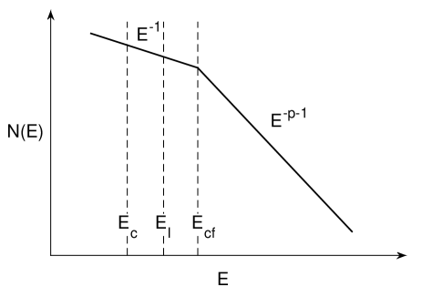
(a) Case (i)

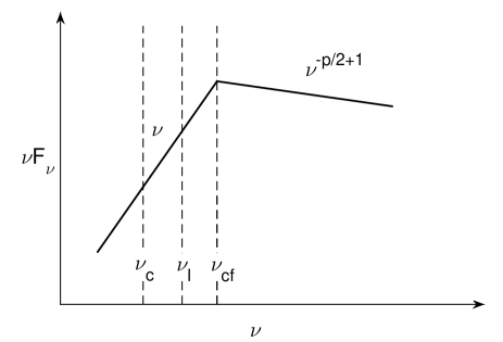
(b) Case (i)

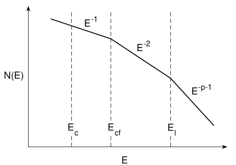
(c) Case (ii)

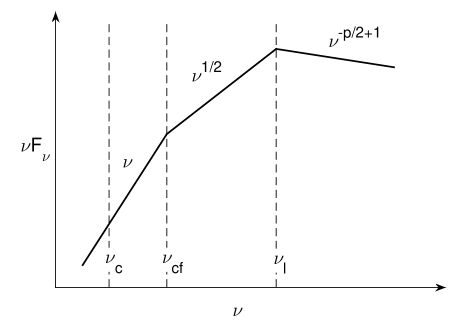
(d) Case (ii)

Figure 1.— The electron energy spectrum ((a) and (c)) under the effects of ASA and synchrotron cooling and the corresponding synchrotron spectrum ((b) and (d)) in Case (i) and Case (ii).

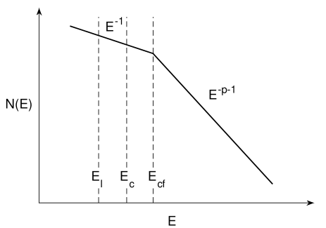
(a) Case (iii)

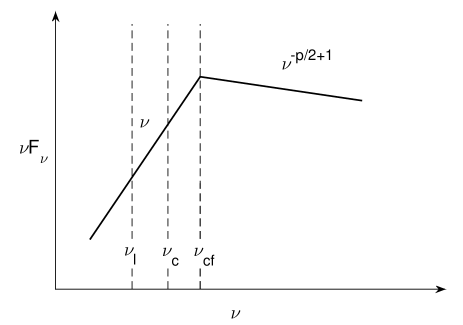
(b) Case (iii)

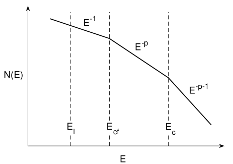
(c) Case (iv)

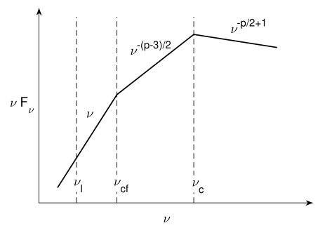
(d) Case (iv)

Figure 2.— The same as Fig. 1 but for Case (iii) and Case (iv).

3. Comparisons between analytical spectral shapes and observed spectra of PWNe

The synchrotron emission of PWNe is characterized by a broad-band spectrum. It typically has a flat radio component with $F_{\nu}\propto\nu^{\alpha}$, where $-0.3\lesssim\alpha\lesssim 0$, and a steep X-ray component with $\alpha\sim-1$ (Chevalier, 2005; Gaensler & Slane, 2006; Reynolds et al., 2017). We apply the above theoretical model to interpreting the spectral shape of the Mouse PWN (Section 3.1) and some other PWNe with well-characterized multi-wavelength spectra (Section 3.2). Here we aim at explaining the overall spectral shapes, rather than providing detailed fits for individual sources.

3.1. Application to the Mouse PWN

Fig. 3 presents the observed multi-wavelength spectrum of G359.23-0.82, a.k.a., the Mouse PWN powered by PSR J1747-2958. Over the radio and X-ray data points taken from Klingler et al. (2018) (hereafter K18), we first assume the spectral shape given in Eq. (12b) corresponding to Case (i) or Case (iii) in Section 2.3. Here we adopt $p=2.18$ according to the fit to the X-ray data in K18. We see that the two spectral segments dominated by the ASA and radiation losses separately match the radio and X-ray data.

The photon energy $E_{\text{ph}}$ is related to the electron Lorentz factor $\gamma_{e}$ by

$$E_{\text{ph}}=\hbar\frac{eB}{m_{e}c}\gamma_{e}^{2}\Gamma,$$ (15)

with $\hbar=h/2\pi$, the Planck constant $h$, the electron charge $e$, the Lorentz factor $\Gamma(\approx 1)$ of the mildly relativistic bulk flow in the PWN (Reynolds et al., 2017). The lowest observed photon energy $E_{\text{ph,m}}=6.2\times 10^{-7}$ eV provides the upper limit of $\gamma_{e,\text{m}}=E_{m}/(m_{e}c^{2})$,

$$\gamma_{e,\text{m,max}}=5.2\times 10^{2}\Big{(}\frac{\Gamma}{1}\Big{)}^{-\frac{1}{2}}\Big{(}\frac{B}{200~{}\mu\text{G}}\Big{)}^{-\frac{1}{2}}\Big{(}\frac{E_{\text{ph,m}}}{6.2\times 10^{-7}~{}\text{eV}}\Big{)}^{\frac{1}{2}}.$$ (16)

Here we adopt the equipartition magnetic field $B\sim 200~{}\mu$G estimated in K18.

The spectral break appears at the photon energy $E_{\text{ph,b}}\approx 9\times 10^{-3}$ eV. It is related to the cutoff electron energy $E_{\text{cf}}=\gamma_{e,\text{cf}}m_{e}c^{2}$ and signifies the balance between acceleration and cooling. So we have

$$\gamma_{e,\text{cf}}=6.2\times 10^{4}\Big{(}\frac{\Gamma}{1}\Big{)}^{-\frac{1}{2}}\Big{(}\frac{B}{200~{}\mu\text{G}}\Big{)}^{-\frac{1}{2}}\Big{(}\frac{E_{\text{ph,b}}}{9\times 10^{-3}~{}\text{eV}}\Big{)}^{\frac{1}{2}}.$$ (17)

It gives the upper limit of the minimum Lorentz factor of injected electrons $\gamma_{e,l}=E_{l}/(m_{e}c^{2})$ in this scenario. It also gives the minimum cooling time for the condition $E_{c}<E_{\text{cf}}$ to be satisfied (Eqs. (8), (10), and (17)),

$$t_{\text{c,min}} =\frac{1}{E_{\text{cf}}\beta}=\frac{1}{\gamma_{e,\text{cf}}m_{e}c^{2}\beta}$$ (18)

$$=9.9\Big{(}\frac{\Gamma}{1}\Big{)}^{\frac{1}{2}}\Big{(}\frac{B}{200~{}\mu\text{G}}\Big{)}^{-\frac{3}{2}}\Big{(}\frac{E_{\text{ph,b}}}{9\times 10^{-3}~{}\text{eV}}\Big{)}^{-\frac{1}{2}}~{}\text{kyr}.$$

Besides, the maximum cooling time $t_{\text{c,max}}$ is given by the spin-down age $t_{\text{sd}}=25.5$ kyr of the pulsar (K18). It corresponds to the electron Lorentz factor (Eqs. (8), (10), and (16)),

$$\gamma_{e,\text{sd}} =\frac{1}{m_{e}c^{2}\beta t_{\text{sd}}}$$ (19)

$$=2.4\times 10^{4}\Big{(}\frac{B}{200~{}\mu\text{G}}\Big{)}^{-2}\Big{(}\frac{t_{\text{sd}}}{25.5~{}\text{kyr}}\Big{)}^{-1} >\gamma_{e,\text{m,max}},$$

implying that the electrons in the Mouse PWN are in the slow cooling regime with $E_{c,\text{min}}>E_{m,\text{max}}$ (see also K18 for the analysis of the cooling regime).

Moreover, $t_{\text{c,min}}$ in Eq. (18) also gives the acceleration timescale of the ASA (Eq. (7)),

$$\tau_{\text{acc}}=a_{A}^{-1}=t_{\text{c,min}}.$$ (20)

We note that $\tau_{\text{acc}}$ in Case (i) or Case (iii) is shorter than $t_{c}$.

Including the tentative infrared point (see Fig. 3 and K18) requires the spectral shape given by Eq. (13c) in Case (ii) or Eq. (14c) in Case (iv). The spectral breaks at lower and higher energies are $E_{\text{ph,b1}}\approx 3.1\times 10^{-4}$ eV, $E_{\text{ph,b2}}\approx 0.15$ eV in Case (ii), and $E_{\text{ph,b1}}\approx 6.9\times 10^{-4}$ eV, $E_{\text{ph,b2}}\approx 0.18$ eV in Case (iv). Similar to the above analysis, these break energies can be used to infer the characteristic $\gamma_{e}$, $t_{\text{c}}$, and $\tau_{\text{acc}}$ (Eqs. (15), (18), and (20)), as shown in Table 1. We see that since the minimum $t_{\text{c}}$ required in Case (ii) is much larger than $t_{\text{sd}}$ of the pulsar, Case (ii) is disfavored.

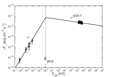
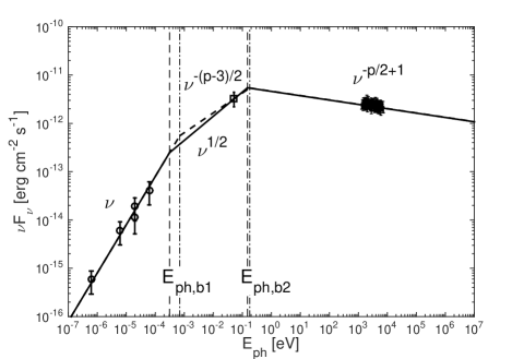
Figure 3.— Our analytical spectral shapes in comparison with the data points of the Mouse PWN taken from K18. Circles, square, and dots represent radio, infrared, and X-ray data, respectively. The spectral shapes are given by Eq. (12b) (solid line) in (a), and Eq. (13c) (solid line) and Eq. (14c) (dashed line) in (b). The vertical lines indicate break energies.

Table 1Characteristic parameters inferred from the spectral breaks of the Mouse PWN

$E_{\text{ph}}$	$E_{\text{ph,m}}$	$E_{\text{ph,b}}$ or $E_{\text{ph,b1}}$	$E_{\text{ph,b2}}$
Case (i) or Case (iii)	$\gamma_{e,\text{m}}\approx 5.2\times 10^{2}$	$\gamma_{e,\text{cf}}=\gamma_{e,l,\text{max}}\approx 6.2\times 10^{4}$, $\tau_{\text{acc}}=t_{\text{c,min}}\approx 9.9$ kyr	—
Case (ii)		$\gamma_{e,\text{cf}}\approx 1.1\times 10^{4}$, $\tau_{\text{acc}}=t_{\text{c,min}}\approx 53.5$ kyr	$\gamma_{e,l}\approx 2.5\times 10^{5}$
Case (iv)		$\gamma_{e,\text{cf}}=\gamma_{e,l,\text{max}}\approx 1.7\times 10^{4}$,$\tau_{\text{acc}}\approx 35.8$ kyr	$t_{\text{c}}\approx 2.2$ kyr

The above comparisons show that our analytical spectral shapes agree well with the observed multi-wavelength spectrum of the Mouse PWN. The ASA and synchrotron cooling in the PWN naturally account for the flatness and steepness of the radio and X-ray spectra ($F_{\nu}$), respectively. More reliable infrared measurements with e.g., HST, JWST, and ALMA are needed to determine the detailed spectral shape at intermediate energies and to distinguish between Case (i) (or Case (iii)) and Case (iv).

3.2. Application to some other PWNe

We next compare our analytical spectral shapes with the synchrotron spectra of some other PWNe to further examine the applicability of our model.

In Fig. 4, we display the synchrotron spectra of 3C 58 (Slane et al., 2008), G21.5-0.9 (Salter et al., 1989), G0.9+0.1 (Tanaka & Takahara, 2011), and N157B (Zhu et al., 2018). We also include the infrared data for 3C 58, but we caution that the observed values are only upper limits (Slane et al., 2008). The X-ray data for G21.5-0.9 and N157B were obtained from Chandra ObsIDs 2873, 3699 3700, 5158, 5159, 5165, 5166, 6070, 6071, 6740, 6741, 8371, 8372 (G21.5–0.9), and 2783 (N157B). The data were reprocessed using the Chandra Interactive Analysis of Observations (CIAO) software version 4.9 and the CXO Calibration Data Base (CALDB) version 4.7.7. All observations were reprocessed with chandra_repro to apply the latest calibrations. We extracted the spectra using specextract and fitted the power-law spectra using the tbabs model of XSPEC (v12.9.1p, which uses absorption cross-sections from Wilms et al. (2000)). For G21.5–0.9 we use a circular $2\farcm 5$ aperture centered on the pulsar, and excluding the bright point source to the South. For N157B, we use a 53^′′ $\times$ 24^′′ extraction region approximately coincident with the brightest radio contour shown in Figure 3 of Chen et al. (2006) and free of thermal supernova remnant (SNR) filaments. In both cases we use background regions located outside the extent of the PWNe/SNRs, and restricted the spectral fits to the 0.5–8 keV range. We verified that our results are not noticeably contaminated by thermal SNR emission by restricting the spectral fits to energies above 2 keV and re-fitting; in both cases the resulting power-law slopes were virtually identical. Our fits to the X-ray data imply $p=1.68$ for G21.5-0.9 and $p=2.6$ for N157B. For 3C 58 and G0.9+0.1, we use $p=2.4$ and $p=2.6$ according to the fits to their X-ray data (Slane et al., 2008; Tanaka & Takahara, 2011).

For 3C 58 and G21.5-0.9, as indicated by the data, we apply the spectral shape in Eq. (13c) (Case (ii)) and that in Eq. (12b) (Case (i) or Case (iii)), respectively. For G0.9+0.1 and N157B, the measurements are insufficient to constrain the detailed spectral form in the intermediate energy range, so we present all possible spectral shapes for comparison with future observations. In all cases, it is clear that the electrons in the PWN should undergo the stochastic acceleration to account for the radio spectrum. The general agreement between our analytical spectral shapes and observed spectra implies the ASA and synchrotron cooling together as a common origin of broad-band synchrotron spectra of PWNe.

The spectral break between radio and X-ray bands or radio and infrared bands is determined by $\tau_{\text{acc}}$ of the ASA. When $\tau_{\text{acc}}$ is sufficiently short for $E_{\text{cf}}$ to be larger than both $E_{c}$ and $E_{l}$, the synchrotron spectrum of a PWN falls in Case (i) or Case (iii). Then we can rewrite Eq. (18) as

$$\Big{(}\frac{\tau_{\text{acc}}}{1~{}\text{kyr}}\Big{)}\Big{(}\frac{B}{100~{}\mu\text{G}}\Big{)}^{\frac{3}{2}}=26.5\Big{(}\frac{\Gamma}{1}\Big{)}^{\frac{1}{2}}\Big{(}\frac{E_{\text{ph,b}}}{10^{-2}~{}\text{eV}}\Big{)}^{-\frac{1}{2}},$$ (21)

and obtain a constraint on $\tau_{\text{acc}}$ and $B$ in the PWN. When $\tau_{\text{acc}}$ is relatively long with $E_{\text{cf}}<E_{l}$ or $E_{\text{cf}}<E_{c}$, the PWN is in Case (ii) or Case (iv). Accordingly, we have

$$\Big{(}\frac{\tau_{\text{acc}}}{1~{}\text{kyr}}\Big{)}\Big{(}\frac{B}{100~{}\mu\text{G}}\Big{)}^{\frac{3}{2}}=837.0\Big{(}\frac{\Gamma}{1}\Big{)}^{\frac{1}{2}}\Big{(}\frac{E_{\text{ph,b1}}}{10^{-5}~{}\text{eV}}\Big{)}^{-\frac{1}{2}}.$$ (22)

If the spectral shape in the infrared band cannot be observationally determined (e.g., G0.9+0.1, N157B), we can still set a constraint on the range of $\tau_{\text{acc}}$ and $B$,

$$26.5\Big{(}\frac{\Gamma}{1}\Big{)}^{\frac{1}{2}}\Big{(}\frac{E_{\text{ph,b}}}{10^{-2}~{}\text{eV}}\Big{)}^{-\frac{1}{2}} \leq\Big{(}\frac{\tau_{\text{acc}}}{1~{}\text{kyr}}\Big{)}\Big{(}\frac{B}{100~{}\mu\text{G}}\Big{)}^{\frac{3}{2}}$$ (23)

$$\leq 837.0\Big{(}\frac{\Gamma}{1}\Big{)}^{\frac{1}{2}}\Big{(}\frac{E_{\text{ph,b1}}}{10^{-5}~{}\text{eV}}\Big{)}^{-\frac{1}{2}}.$$

In Table 2, we list the values of $E_{\text{ph,b}}$ and $E_{\text{ph,b1}}$ of the above PWNe. For G0.9+0.1 and N157B, we can only provide the lower limit of $E_{\text{ph,b1}}$ due to the insufficient data points. By using the estimated magnetic field strength $B_{\text{eq}}$ under the assumption of equipartition between particle and magnetic energies (see Table 2), in Fig. 5 we present the corresponding $\tau_{\text{acc}}$ (Eqs. (21) and (22)) or the range of $\tau_{\text{acc}}$ (Eq. (23)) inferred from the spectral breaks of the PWNe. Empirically, we see that $\tau_{\text{acc}}$ of different PWNe are basically within the range confined by Eq. (23).

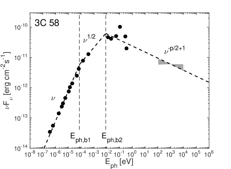
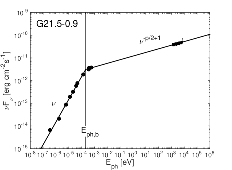
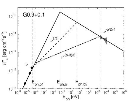
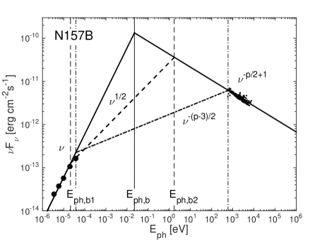
Figure 4.— Our analytical spectral shapes (solid line: Eq. (12b), dashed line: Eq. (13c), dash-dotted line: Eq. (14c)) in comparison with the observed synchrotron spectra of PWNe. Vertical lines indicate break energies.

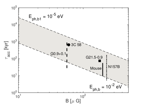
Figure 5.— $\tau_{\text{acc}}$ vs. $B_{\text{eq}}$ of the PWNe. The shaded region is bounded by Eq. (23).

Table 2Parameters of the PWNe

PWNe	Mouse	3C 58	G21.5-0.9	G0.9+0.1	N157B
$E_{\text{ph,b}}$ [eV]	$9.0\times 10^{-3}$	—	$2.1\times 10^{-4}$	$5.8\times 10^{-2}$	$2.2\times 10^{-2}$
$E_{\text{ph,b1,min}}$ [eV]	$3.1\times 10^{-4}$	$7.3\times 10^{-5}$	—	$5.0\times 10^{-5}$	$2.1\times 10^{-5}$
$B_{\text{eq}}$ [$\mu$G]	$200$(1)	$60$(2)	$180$(3)	$56$(4)	$230$(5)

• K18.

• Reynolds & Aller (1988).

• Safi-Harb et al. (2001).

• Dubner et al. (2008).

• Wang et al. (2001)

4. Discussion

Turbulence is believed to be present in PWNe, but its origin and properties are unclear. Besides the magnetic reconnection under consideration here, other possible sources of turbulence include, e.g., the Rayleigh-Taylor instability induced by the interaction between the PWN and the supernova remnant (Chevalier & Gull, 1975; Porth et al., 2014a), the dynamical instability of the PW’s oscillating magnetic field (Zrake, 2016), the Weibel instability (Weibel, 1959; Sironi & Spitkovsky, 2011), the large-scale shear flows in the PWN (Komissarov & Lyubarsky, 2004). For bow-shock PWNe, an additional source of turbulence can be the Richtmyer-Meshkov instability induced by their interaction with interstellar density fluctuations (Giacalone & Jokipii, 2007). As a more general mechanism to generate turbulence, the magnetic reconnection is dynamically coupled with turbulence and naturally converts magnetic energy to turbulent energy. The generated turbulence allows efficient dissipation of magnetic energy through turbulent reconnection in the PW, and further ASA of the electrons in the PWN.

Non-adiabatic stochastic acceleration including the gyroresonance and transit time damping (TTD) can also result in a hard electron spectrum (Melrose, 1969). As is known, the gyroresonance with Alfvén modes is inefficient due to the turbulence anisotropy (Chandran, 2000; Yan & Lazarian, 2002), while TTD with compressive fast and slow modes can be alternative stochastic acceleration mechanisms (Yan & Lazarian, 2008; Xu & Lazarian, 2018). However, only a small fraction of turbulent energy is contained in compressive modes in compressible MHD turbulence (Cho & Lazarian, 2002; Kowal & Lazarian, 2010). Moreover, fast modes are usually subjected to severe plasma damping effects (Yan & Lazarian, 2004), and TTD with slow modes also suffers the turbulence anisotropy (Xu & Lazarian, 2018). We note that the turbulence anisotropy is scale-dependent (Cho & Lazarian, 2003). Even at a low magnetization in outer regions of PWNe, the turbulent eddies at the small resonant scale are still highly anisotropic. Therefore, when the pitch-angle scattering and non-adiabatic stochastic acceleration are inefficient, the ASA can account for the stochastic acceleration in PWNe. Since the largest eddies are most effective in ASA, its efficiency does not depend on the turbulence spectral slope. We find numerical evidence for the ASA in both MHD simulations (Lynn et al., 2012) and kinetic particle-in-cell simulations (Dahlin et al., 2017). Obviously, in a situation where the pitch-angle scattering is efficient and thus the adiabatic invariance is violated, the ASA is suppressed.

The ASA occurs when the Larmor radius $r_{L}$ of electrons is much smaller than the characteristic length scale of turbulent magnetic fields. The largest $r_{L}$ of the stochastically accelerated electrons corresponding to $E_{\text{ph,b}}$ is (Eq. (17))

$$r_{L} =\frac{\gamma_{e,\text{cf}}m_{e}c^{2}}{eB}$$ (24)

$$=1.6\times 10^{12}\Big{(}\frac{\Gamma}{1}\Big{)}^{-\frac{1}{2}}\Big{(}\frac{B}{100~{}\mu\text{G}}\Big{)}^{-\frac{3}{2}}\Big{(}\frac{E_{\text{ph,b}}}{10^{-2}~{}\text{eV}}\Big{)}^{\frac{1}{2}}~{}\text{cm}.$$

It is indeed small compared with the characteristic turbulence scale of the order of $0.1$ pc suggested by polarization observations of PWNe (e.g., Yusef-Zadeh & Gaensler 2005; Moran et al. 2013; Ma et al. 2016). Given the turbulence scale $l_{\text{tur}}$ and $\tau_{\text{acc}}$, we can also estimate the turbulent speed at $l_{\text{tur}}$ (Eqs. (3), (18), and (20))

$$u_{\text{tur}} =\xi^{-1}l_{\text{tur}}\tau_{\text{acc}}^{-1}$$ (25)

$$=3.7\Big{(}\frac{\xi}{1}\Big{)}^{-1}\Big{(}\frac{\Gamma}{1}\Big{)}^{-\frac{1}{2}}\Big{(}\frac{B}{100~{}\mu\text{G}}\Big{)}^{\frac{3}{2}}\Big{(}\frac{E_{\text{ph,b}}}{10^{-2}~{}\text{eV}}\Big{)}^{\frac{1}{2}}$$

$$~{}~{}~{}~{}~{}~{}\Big{(}\frac{l_{\text{tur}}}{0.1~{}\text{pc}}\Big{)}~{}\text{km s${}^{-1}$}.$$

If we assume that the interstellar turbulence driven by supernova explosions has $L_{i}\sim 100$ pc and the turbulent speed $V_{L}\sim 10$ km s^-1 at $L_{i}$ (Kaplan & Pikelner, 1970), then according to the Kolmogorov scaling (Armstrong et al., 1995; Chepurnov & Lazarian, 2010), the turbulent speed in the interstellar medium at $0.1$ pc is $v_{l}=V_{L}(l/L_{i})^{1/3}\sim 1$ km s^-1. It implies that the turbulence level in a PWN can be comparable to the surrounding interstellar turbulence.

We have analyzed the synchrotron spectra of both bow-shock PWN (Mouse) and PWNe supernova remnants (3C 58, G21.5-0.9, G0.9+0.1, N157B). Despite their possibly different interaction with ambient media, all PWNe exhibit broken power-law spectra with a flat radio component ($F_{\nu}$) and a steeper X-ray component. This common feature implies that both stochastic acceleration and synchrotron cooling of electrons generally exist in different types of PWNe. Relativistic MHD simulations of PWNe also support that radio emitting particles undergo a local re-acceleration process in the nebula by the interaction with turbulence (Olmi et al., 2014, 2016).

The ASA is a promising mechanism of particle re-acceleration to explain the flat $F_{\nu}$ spectra of different sources. Besides gamma-ray bursts discussed in earlier studies (Xu & Zhang, 2017; Xu et al., 2018) and PWNe considered here, it can also be applicable to e.g. radio galaxies, blazars, which will be investigated in our future work.

5. Summary

Recent advances in the theoretical understanding of MHD turbulence bring us new insights in basic physical processes related to PWNe.

We suggested that the magnetic reconnection in the PW inevitably falls in the turbulent reconnection regime and thus is efficient in converting the magnetic energy to the particle energy.

We focused on the re-acceleration of particles in the PWN through the mechanism ASA. The ASA acts to flatten the injected energy spectrum of electrons. It results in a flat radio spectrum (in $F_{\nu}$) of the photons radiated downstream of the termination shock. The steeper X-ray spectrum can be simply attributed to synchrotron cooling, which is dominant at high energies. At intermediate energies, the detailed spectral shape depends on the acceleration timescale of the ASA.

Our analytical spectral shapes incorporating both the ASA and synchrotron cooling generally agree well with the observed broad-band synchrotron spectra of PWNe. The spectral breaks can be used to constrain the acceleration timescale of the ASA and the magnetic field strength in the PWN (see Fig. 5). They can also provide valuable information on the cooling time and injected electron energy (see Table 1).

References

- Abdo et al. (2011) Abdo, A. A., et al. 2011, Science, 331, 739
- Armstrong et al. (1995) Armstrong, J. W., Rickett, B. J., & Spangler, S. R. 1995, ApJ, 443, 209
- Arons (2002) Arons, J. 2002, in Astronomical Society of the Pacific Conference Series, Vol. 271, Neutron Stars in Supernova Remnants, ed. P. O. Slane & B. M. Gaensler, 71
- Band et al. (1993) Band, D., et al. 1993, ApJ, 413, 281
- Begelman (1998) Begelman, M. C. 1998, ApJ, 493, 291
- Begelman & Li (1992) Begelman, M. C., & Li, Z.-Y. 1992, ApJ, 397, 187
- Bogovalov et al. (2005) Bogovalov, S. V., Chechetkin, V. M., Koldoba, A. V., & Ustyugova, G. V. 2005, MNRAS, 358, 705
- Brunetti & Lazarian (2007) Brunetti, G., & Lazarian, A. 2007, MNRAS, 378, 245
- Brunetti & Lazarian (2016) —. 2016, MNRAS, 458, 2584
- Chandran (2000) Chandran, B. D. G. 2000, Physical Review Letters, 85, 4656
- Chen et al. (2006) Chen, Y., Wang, Q. D., Gotthelf, E. V., Jiang, B., Chu, Y.-H., & Gruendl, R. 2006, ApJ, 651, 237
- Chepurnov & Lazarian (2010) Chepurnov, A., & Lazarian, A. 2010, ApJ, 710, 853
- Chevalier (2005) Chevalier, R. A. 2005, ApJ, 619, 839
- Chevalier & Gull (1975) Chevalier, R. A., & Gull, T. R. 1975, ApJ, 200, 399
- Cho & Lazarian (2002) Cho, J., & Lazarian, A. 2002, Physical Review Letters, 88, 245001
- Cho & Lazarian (2003) —. 2003, MNRAS, 345, 325
- Coroniti (1990) Coroniti, F. V. 1990, ApJ, 349, 538
- Dahlin et al. (2017) Dahlin, J. T., Drake, J. F., & Swisdak, M. 2017, Physics of Plasmas, 24, 092110
- de Gouveia dal Pino & Lazarian (2005) de Gouveia dal Pino, E. M., & Lazarian, A. 2005, A&A, 441, 845
- del Valle et al. (2016) del Valle, M. V., de Gouveia Dal Pino, E. M., & Kowal, G. 2016, MNRAS, 463, 4331
- Del Zanna et al. (2016) Del Zanna, L., Papini, E., Landi, S., Bugli, M., & Bucciantini, N. 2016, MNRAS, 460, 3753
- Deng et al. (2015) Deng, W., Li, H., Zhang, B., & Li, S. 2015, ApJ, 805, 163
- Dubner et al. (2008) Dubner, G., Giacani, E., & Decourchelle, A. 2008, A&A, 487, 1033
- East et al. (2015) East, W. E., Zrake, J., Yuan, Y., & Blandford, R. D. 2015, Physical Review Letters, 115, 095002
- Fleishman & Bietenholz (2007) Fleishman, G. D., & Bietenholz, M. F. 2007, MNRAS, 376, 625
- Gaensler & Slane (2006) Gaensler, B. M., & Slane, P. O. 2006, ARA&A, 44, 17
- Giacalone & Jokipii (1999) Giacalone, J., & Jokipii, J. R. 1999, ApJ, 520, 204
- Giacalone & Jokipii (2007) —. 2007, ApJ, 663, L41
- Goldreich & Sridhar (1995) Goldreich, P., & Sridhar, S. 1995, ApJ, 438, 763
- Guo et al. (2017) Guo, X., Mao, J., & Wang, J. 2017, ApJ, 843, 23
- Kaplan & Pikelner (1970) Kaplan, S. A., & Pikelner, S. B. 1970, The interstellar medium (Cambridge: Harvard University Press)
- Kardashev (1962) Kardashev, N. S. 1962, AZh, 39, 393
- Kennel & Coroniti (1984) Kennel, C. F., & Coroniti, F. V. 1984, ApJ, 283, 694
- Klingler et al. (2018) Klingler, N., Kargaltsev, O., Pavlov, G. G., Ng, C.-Y., Beniamini, P., & Volkov, I. 2018, ApJ, 861, 5
- Komissarov & Lyubarsky (2004) Komissarov, S. S., & Lyubarsky, Y. E. 2004, MNRAS, 349, 779
- Kowal et al. (2011) Kowal, G., de Gouveia Dal Pino, E. M., & Lazarian, A. 2011, ApJ, 735, 102
- Kowal et al. (2012) —. 2012, Physical Review Letters, 108, 241102
- Kowal et al. (2017) Kowal, G., Falceta-Gonçalves, D. A., Lazarian, A., & Vishniac, E. T. 2017, ApJ, 838, 91
- Kowal & Lazarian (2010) Kowal, G., & Lazarian, A. 2010, ApJ, 720, 742
- Kowal et al. (2009) Kowal, G., Lazarian, A., Vishniac, E. T., & Otmianowska-Mazur, K. 2009, in Revista Mexicana de Astronomia y Astrofisica Conference Series, Vol. 36, Revista Mexicana de Astronomia y Astrofisica Conference Series, 89–96
- Lazarian & Vishniac (1999) Lazarian, A., & Vishniac, E. T. 1999, ApJ, 517, 700
- Lazarian et al. (2018) Lazarian, A., Zhang, B., & Xu, S. 2018, arXiv:1801.04061
- Lynn et al. (2012) Lynn, J. W., Parrish, I. J., Quataert, E., & Chandran, B. D. G. 2012, ApJ, 758, 78
- Lyubarsky & Kirk (2001) Lyubarsky, Y., & Kirk, J. G. 2001, ApJ, 547, 437
- Ma et al. (2016) Ma, Y. K., Ng, C.-Y., Bucciantini, N., Slane, P. O., Gaensler, B. M., & Temim, T. 2016, ApJ, 820, 100
- Maron & Goldreich (2001) Maron, J., & Goldreich, P. 2001, ApJ, 554, 1175
- Melrose (1969) Melrose, D. B. 1969, Ap&SS, 5, 131
- Meszaros & Rees (1993) Meszaros, P., & Rees, M. J. 1993, ApJ, 418, L59
- Mignone et al. (2013) Mignone, A., Striani, E., Tavani, M., & Ferrari, A. 2013, MNRAS, 436, 1102
- Mizuno et al. (2011) Mizuno, Y., Lyubarsky, Y., Nishikawa, K.-I., & Hardee, P. E. 2011, ApJ, 728, 90
- Moran et al. (2013) Moran, P., Shearer, A., Mignani, R. P., Słowikowska, A., De Luca, A., Gouiffès, C., & Laurent, P. 2013, MNRAS, 433, 2564
- Olmi et al. (2014) Olmi, B., Del Zanna, L., Amato, E., Bandiera, R., & Bucciantini, N. 2014, MNRAS, 438, 1518
- Olmi et al. (2016) Olmi, B., Del Zanna, L., Amato, E., Bucciantini, N., & Mignone, A. 2016, Journal of Plasma Physics, 82, 635820601
- Parker (1957) Parker, E. N. 1957, J. Geophys. Res., 62, 509
- Pavlov et al. (2003) Pavlov, G. G., Teter, M. A., Kargaltsev, O., & Sanwal, D. 2003, ApJ, 591, 1157
- Pohl et al. (2005) Pohl, M., Yan, H., & Lazarian, A. 2005, ApJ, 626, L101
- Porth et al. (2014a) Porth, O., Komissarov, S. S., & Keppens, R. 2014a, MNRAS, 443, 547
- Porth et al. (2014b) —. 2014b, MNRAS, 438, 278
- Preece et al. (2000) Preece, R. D., Briggs, M. S., Mallozzi, R. S., Pendleton, G. N., Paciesas, W. S., & Band, D. L. 2000, ApJS, 126, 19
- Rees & Gunn (1974) Rees, M. J., & Gunn, J. E. 1974, MNRAS, 167, 1
- Reynolds & Aller (1988) Reynolds, S. P., & Aller, H. D. 1988, ApJ, 327, 845
- Reynolds et al. (2017) Reynolds, S. P., Pavlov, G. G., Kargaltsev, O., Klingler, N., Renaud, M., & Mereghetti, S. 2017, Space Sci. Rev., 207, 175
- Rybicki & Lightman (1979) Rybicki, G. B., & Lightman, A. P. 1979, Radiative processes in astrophysics
- Safi-Harb et al. (2001) Safi-Harb, S., Harrus, I. M., Petre, R., Pavlov, G. G., Koptsevich, A. B., & Sanwal, D. 2001, ApJ, 561, 308
- Salter et al. (1989) Salter, C. J., Reynolds, S. P., Hogg, D. E., Payne, J. M., & Rhodes, P. J. 1989, ApJ, 338, 171
- Sari et al. (1998) Sari, R., Piran, T., & Narayan, R. 1998, ApJ, 497, L17
- Sironi & Spitkovsky (2011) Sironi, L., & Spitkovsky, A. 2011, ApJ, 741, 39
- Slane et al. (2008) Slane, P., Helfand, D. J., Reynolds, S. P., Gaensler, B. M., Lemiere, A., & Wang, Z. 2008, ApJ, 676, L33
- Sweet (1958) Sweet, P. A. 1958, in IAU Symposium, Vol. 6, Electromagnetic Phenomena in Cosmical Physics, ed. B. Lehnert, 123
- Takamoto et al. (2015) Takamoto, M., Inoue, T., & Lazarian, A. 2015, ApJ, 815, 16
- Tanaka & Asano (2017) Tanaka, S. J., & Asano, K. 2017, ApJ, 841, 78
- Tanaka & Takahara (2011) Tanaka, S. J., & Takahara, F. 2011, ApJ, 741, 40
- Tavani et al. (2011) Tavani, M., et al. 2011, Science, 331, 736
- Wang et al. (2001) Wang, Q. D., Gotthelf, E. V., Chu, Y.-H., & Dickel, J. R. 2001, ApJ, 559, 275
- Weibel (1959) Weibel, E. S. 1959, Physical Review Letters, 2, 83
- Wilms et al. (2000) Wilms, J., Allen, A., & McCray, R. 2000, ApJ, 542, 914
- Xu & Lazarian (2016) Xu, S., & Lazarian, A. 2016, ApJ, 833, 215
- Xu & Lazarian (2018) —. 2018, ApJ, 868, 36
- Xu et al. (2016) Xu, S., Yan, H., & Lazarian, A. 2016, ApJ, 826, 166
- Xu et al. (2018) Xu, S., Yang, Y.-P., & Zhang, B. 2018, ApJ, 853, 43
- Xu & Zhang (2017) Xu, S., & Zhang, B. 2017, ApJ, 846, L28
- Yan & Lazarian (2002) Yan, H., & Lazarian, A. 2002, Physical Review Letters, 89, B1102+
- Yan & Lazarian (2004) —. 2004, ApJ, 614, 757
- Yan & Lazarian (2008) —. 2008, ApJ, 673, 942
- Yan et al. (2008) Yan, H., Lazarian, A., & Petrosian, V. 2008, ApJ, 684, 1461
- Yusef-Zadeh & Gaensler (2005) Yusef-Zadeh, F., & Gaensler, B. M. 2005, Advances in Space Research, 35, 1129
- Zhang & Yan (2011) Zhang, B., & Yan, H. 2011, ApJ, 726, 90
- Zhu et al. (2018) Zhu, B.-T., Zhang, L., & Fang, J. 2018, A&A, 609, A110
- Zrake (2016) Zrake, J. 2016, ApJ, 823, 39
- Zrake & East (2016) Zrake, J., & East, W. E. 2016, ApJ, 817, 89