ST-GRAT: A Novel Spatio-temporal Graph Attention Network for Accurately Forecasting Dynamically Changing Road Speed

Abstract.

Predicting road traffic speed is a challenging task due to different types of roads, abrupt speed change and spatial dependencies between roads; it requires the modeling of dynamically changing spatial dependencies among roads and temporal patterns over long input sequences. This paper proposes a novel spatio-temporal graph attention (ST-GRAT) that effectively captures the spatio-temporal dynamics in road networks. The novel aspects of our approach mainly include spatial attention, temporal attention, and spatial sentinel vectors. The spatial attention takes the graph structure information (e.g., distance between roads) and dynamically adjusts spatial correlation based on road states. The temporal attention is responsible for capturing traffic speed changes, and the sentinel vectors allow the model to retrieve new features from spatially correlated nodes or preserve existing features. The experimental results show that ST-GRAT outperforms existing models, especially in difficult conditions where traffic speeds rapidly change (e.g., rush hours). We additionally provide a qualitative study to analyze when and where ST-GRAT tended to make accurate predictions during rush-hour times.

ACM Reference Format:
Cheonbok Park, Chunggi Lee, Hyojin Bahng, Yunwon Tae, Seungmin Jin, Kihwan Kim, Sungahn Ko, and Jaegul Choo. 2020. ST-GRAT: A Novel Spatio-temporal Graph Attention Network for Accurately Forecasting Dynamically Changing Road Speed. In Proceedings of the 29th ACM International Conference on Information and Knowledge Management (CIKM ’20), October 19–23, 2020, Virtual Event, Ireland. ACM, NY, NY, USA, 10 pages. https://doi.org/10.1145/3340531.3411940

1. Introduction

Predicting traffic speed is a challenging task, as a prediction method needs not only to find innate spatial-temporal dependencies among roads, but also needs to understand how these dependencies change over time and influence other traffic conditions. For example, when a road is congested, there is a high chance that its neighboring roads are also congested. Moreover, roads in residential areas tend to have different traffic patterns compared to those surrounding industrial complexes (Lee et al., 2019).

Numerous deep learning models (Zhao et al., 2017; Pan et al., 2018) have been proposed for traffic speed prediction based on graph convolution neural networks (GCNNs) with recurrent neural networks (RNNs), outperforming conventional approaches (Vlahogianni et al., 2014). For example, a diffusion convolution recurrent neural network (DCRNN) (Li et al., 2018) combines diffusion convolution (Atwood and Towsley, 2016) with an RNN and demonstrates improved prediction accuracy. Graph WaveNet (Wu et al., 2019) adapts diffusion convolution, incorporates a self-adaptive adjacency matrix, and uses dilated convolution for achieving state-of-the-art performance. However, the models assume fixed spatial dependencies among roads, so that they compute spatial dependencies once and use the computed dependencies all the time without considering dynamically changing traffic conditions.

To address this issue, recent models (Zhang et al., 2018; Zheng et al., 2019) utilize multi-head attention (Vaswani et al., 2017) to model spatial dependencies. Despite efforts, they are only partial solutions, as they do not consider overall graph structure information (e.g., distances, connections and directions between nodes), which can play an important role in deciding which road to attend. In summary, any other approaches do not consider both of dynamically adjusting attention weights and the graph structure information.

Many models employ recurrent neural networks (RNNs) for temporal modeling (e.g., DCRNN (Li et al., 2018), GaAN (Zhang et al., 2018)). However, RNNs have a limitation in that they cannot directly access past features in long input sequences, which implies ineffectiveness in modeling temporal dependencies (Wu et al., 2019). Attention-based models can be an alternative to resolve the issue in the RNN-based temporal modeling, directly accessing past information in the long input sequences. However, existing attention models do not consider dynamic temporal dependencies among roads. For example, there are cases where road speed can be best predicted by attending the target roads. However, existing models with attention do not consider these cases, so that they always retrieve new information from neighbor nodes, even in unnecessary cases.

In this work, we propose a novel spatio-temporal graph attention network (ST-GRAT) for predicting traffic speed that addresses aforementioned weaknesses. First, we design a spatial attention module to model the spatial dependencies by capturing both road speed changes and graph structure information, based on our proposed diffusion prior, directed heads, and distance embedding. Second, we encode temporal dependencies by using attention to directly access distant relevant features of input sequences without any restriction and to effectively capture sudden fluctuating temporal dynamics. Third, to avoid attending unrelated roads that are not helpful for prediction, we newly design ‘spatial sentinel’ key and value vectors, motivated by the sentinel mixture model (Merity et al., 2017; Lu et al., 2016). Guided by the sentinel vectors, ST-GRAT dynamically decides to use new information of other roads or focus on existing encoded features. The experimental results indicate that ST-GRAT achieves state-of-the-art performance, especially in short-term prediction. We also confirm that ST-GRAT is better than existing models at predicting traffic speeds in situations where the road speeds are abruptly changing (e.g., rush hours). Moreover, compared to existing methods, our model shows an interptetable ability by using the self-attention mechanism with the sentinel vectors. In the qualitative study, we conduct an interpretation of our trained model by visualizing when and where the model directed its attention based on different traffic conditions. Lastly, we present in-depth alalyses on how the newly designed components dynamically capture spatio-temporal dependencies.

The contributions of this work include:

• ST-GRAT, which consists of entire self-attention mechanisms to dynamically captures both spatial and temporal dependencies of input sequences over time.

• A newly proposed self-attention module with the sentinel vectors that help the model decide to focus on existing encoded features, instead of unnecessary attending other roads,

• A spatial module that uses diffusion prior and directed heads to effectively encode graph structure,

• Quantitative experiments and comparisons with state-of-the art models on the two real-world datasets, including the different time ranges and abruptly changing time ranges (e.g., rush hours), and

• In-depth analysis and interpretation on how ST-GRAT works in varying traffic conditions

2. Related Work

In this section, we review previous approaches regarding traffic prediction and attention models.

2.1. Approaches for Traffic Forecasting

Deep learning models for traffic prediction usually leverage spatial and temporal dependencies of the road traffic. The graph convolution neural network (GCNN) (Kipf and Welling, 2016) have been popular for spatial relationship modeling. Given a road network, it aggregates adjacent node information into features based on convolution coefficients. These coefficients are computed by spatial information (e.g., the distance between nodes). RNNs and their variants are combined with the encoded spatial relationship to model temporal dependencies (e.g., speed sequences) (Yu et al., 2018).

As modeling spatial correlation is a key factor for improving prediction performance, researchers have proposed new approaches for effective spatial correlation modeling. For example, DCRNN  (Li et al., 2018) combines diffusion convolution (Atwood and Towsley, 2016) and recurrent neural networks to model spatial and temporal dependencies. Graph WaveNet (Wu et al., 2019) also adapts diffusion convolution in spatial modeling, but it is different from DCRNN, as it 1) considers both connected and unconnected nodes in the modeling process, and 2) uses dilated convolution (van den Oord et al., [n.d.]) to learn long sequences of data.

Nonetheless, existing approaches use constant coefficients, which are computed once and applied to all traffic conditions. However, the fixed coefficients may result in inaccuracies when spatial correlation is variable (e.g., abrupt speed changes). Compared to existing models, ST-GRAT improves accuracy by dynamically adjusting the coefficients of neighboring nodes based on their present states and more spatial information (e.g., distance, node connectivity, flow direction).

2.2. Attention Models

Attention-based neural networks are widely used for sequence-to-sequence modeling, such as machine translation and natural language processing (NLP) tasks (Cho et al., 2014; Xu et al., 2015; Lin et al., 2017; Seo et al., 2016). Vaswani et al. propose a novel self-attention network called Transformer (Vaswani et al., 2017), which is able to dynamically capture diverse syntactic and semantic features of the given context by using multi-head self-attention heads. The self-attention mechanism has additional advantages compared to conventional long-short-term memory (LSTM) (Hochreiter and Schmidhuber, 1997) in that its process can be easily paralleled, and it directly attends to related input items regardless of the coverage of the receptive field. Due to these advantages, Transformer has contributed to many other NLP tasks for improving accuracy (Radford et al., 2019; Devlin et al., 2019). Another study (Velickovic et al., 2018) used the self-attention network for graph data, demonstrating that the attention networks outperform the GCNN model. Zhang et al. (Zhang et al., 2018) propose a graph attention network, replacing the diffusion convolution operation in DCRNN (Li et al., 2018) with the gating attention. These models show that the graph attention model does not lag behind the GCNN-based model in the spatio-temporal task.

While previous models can be used for replacing GCNN-based spatial modeling, they all have a drawback; they do not consider the information embedded in the graph structure (such as distances, connectivity, and flow directions between nodes) in their spatial dependency modeling processes in deciding when and where to attend. Compared to previous models, ST-GRAT has a novel spatial attention mechanism that can consider all of the mentioned graph structure information.

3. Proposed Approach

In this section, we define the traffic forecasting problem and describe our spatio-temporal graph attention network.

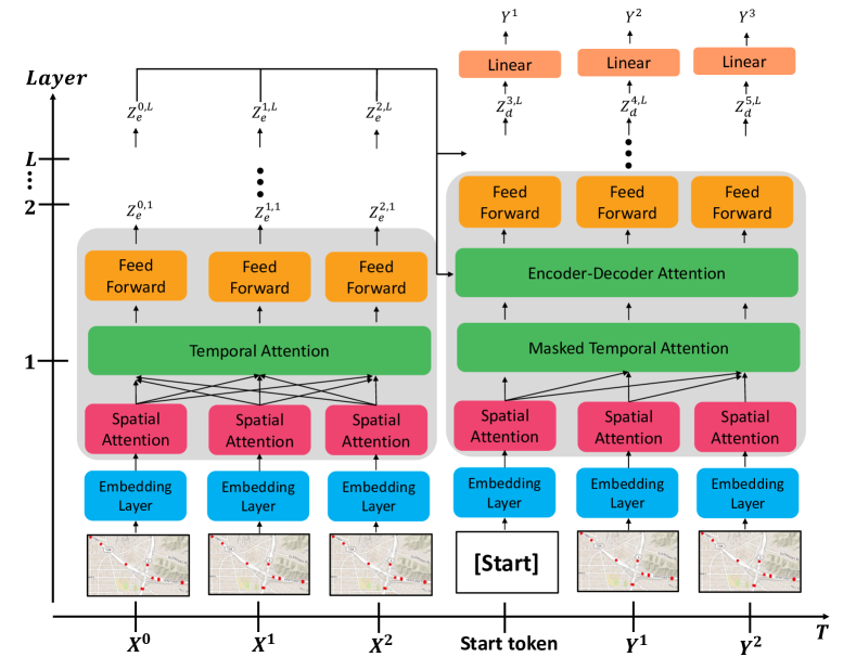
Figure 1. Overall architecture of ST-GRAT. The $x$ and $y$ axes indicate the time and the number of the layers, respectively. The left-half block is the $L$-stacked encoder while the right-half block is the $L$ stacked decoder. We use a special token, ‘[Start]’, to represent the starting point in a decoding stage.

3.1. Problem Setting for Traffic Speed Forecasting

We aim to predict the future traffic speed at each sensor location. We define the input graph as $\mathcal{G}=(\mathcal{V},\mathcal{E},\mathcal{A})$, where $\mathcal{V}$ is the set of all the different sensor nodes, ($|\mathcal{V}|=N$), $\mathcal{E}$ is the set of edges, and $\mathcal{A}\in\mathbb{R}^{N\times N}$ is a weighted adjacency matrix. The matrix $\mathcal{A}$ includes two types of proximity information in the road network: connectivity and edge weights. Connectivity indicates whether two nodes are directly connected or not. Edge weights are comprised of the distance and direction of the edges between two connected nodes. This proximity information refers to the overall structure on a given graph including connectivity, edge directions, and distances of the entire nodes.

We denote $X^{\left(t\right)}\in\mathbb{R}^{N\times 2}$ as the input feature matrix at time $t$, where $N$ is the number of nodes and $2$ is the number of features (the velocity and the timestamp). Following the conventional traffic forecasting problem definition, our problem is to learn a mapping function $f$ that predicts the speed of the next $T$ time steps ($Y=[X^{\left(t+1\right)}_{:,0},\cdots,X^{\left(t+T\right)}_{:,0}]$), given the previous $T$ input speeds in a sequence ($X=[X^{\left(t-T+1\right)},\cdots,X^{\left(t\right)}]$), and graph $\mathcal{G}$, i.e., $Y=f(X,\mathcal{G})$. To solve this sequence-to-sequence learning problem, we utilize an encoder-decoder architecture, as shown in Fig. 1 described in the following sections.

3.2. Encoder Architecture

Given a sequence of observations, $X$, the encoder consists of spatial attention and temporal attention for predicting the future sequence $Y$. As shown in Fig. 1, a single encoder layer consists of three sequential sub-layers: the spatial attention layer, the temporal attention layer, and the point-wise feed-forward neural networks. The spatial attention layer attends to neighbor nodes spatially correlated to the center node at each time-step, while the temporal attention layer attends to individual nodes and focuses on different time steps of a given input sequence. The position-wise feed-forward networks create high-level features that integrate information from the two attention layers. These layers consist of two sequential fully connected networks with GELU (Hendrycks and Gimpel, 2016) activation function.

The encoder has a skip-connection to bypass the sub-layer, and we employ layer normalization (Ba et al., 2016) and dropout after each sub-layer to improve the generalization performance. The overall encoder architecture is a stack of an embedding layer and four ($L=4$) identical encoder layers. The encoder transforms the spatial and temporal dependencies of an input signal into a hidden representation vector, which is used later for attention layers in the decoder.

3.3. Embedding Layer

Unlike GCNN-based models, attention-based GNNs (Velickovic et al., 2018; Zhang et al., 2018) mainly utilize connectivity between nodes. However, conventional models do not consider proximity information in their modeling process. To incorporate the proximity information, the embedding layer in ST-GRAT takes a pre-trained node-embedding vector generated by LINE (Tang et al., 2015). The node-embedding features are used to compute spatial attention, which will be further discussed in the following section.

The embedding layer also performs positional embedding to acquire the order of input sequences. Unlike previous methods that use a recurrent or convolutional layer for sequence modeling, we follow the positional encoding scheme of the Transformer (Vaswani et al., 2017).We apply residual skip connections to prevent the vanishing effect of embedded features that can occur as the number of encoder or decoder layers increases. We concatenate each node embedding result with the node features and then project the concatenated features onto $d_{model}$. Lastly, we add the positional encoding vector to each time step.

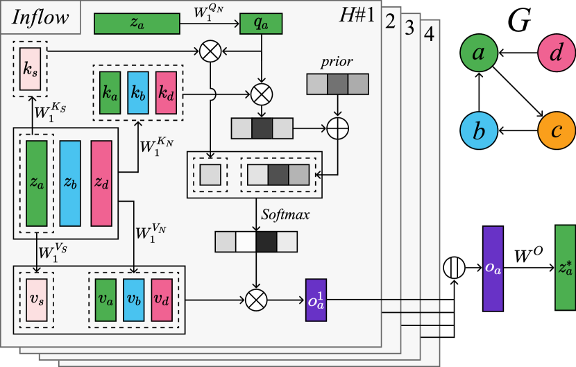
Figure 2. The proposed spatial attention mechanism. In this example, the inflow spatial attention takes query, key, and value vectors, $q$, $k$, and $v$, respectively. $k_{s}$ and $v_{s}$ indicate a sentinel key and value vector. $z^{*}$ represents the output of multi-head attention, and $H\#$ is an indicator of the heads. Lastly, $\oplus$, $\otimes$, and $\parallel$ indicate the element-wise sum, the matrix multiplication, and the concatenation operation, respectively.

3.4. Spatial Attention

Fig. 2 shows the proposed spatial attention, which consists of multiple inflow attention heads (odd head indices) and outflow attention heads (even head indices). Previous attention-based GNNs (Zhang et al., 2018; Velickovic et al., 2018) define spatial correlation in an undirected manner. They calculate attention with respect to all neighbor nodes without considering their direction in a road network. In contrast, our model differentiates neighbor nodes by directions of attention heads. Specifically, we divide the attention heads–i.e., odd indices are responsible for inflow nodes, even indices are responsible for outflow nodes—which allows the model to attend to different information for each of inflow and outflow traffic. Fig. 2 shows the inflow attention head example, which attends only inflow nodes and its node.

We denote the encoder hidden states as $\mathcal{Z}=[z_{i},\cdots,z_{N}]$, where $z_{i}\in\mathcal{R}^{d_{model}}$ is the hidden state of the $i$-th node. We denote the set of the $i$-th node and its neighbor nodes as $\mathcal{N}_{i}$. We define the dimensions of the query, key, and value vectors as $d_{q}=d_{k}=d_{v}=d_{model}/H$, respectively, where $H$ is the number of attention head in multi-head self-attention.

To extract diverse high-level features from multiple attention heads, we project the current node onto a query space and $\mathcal{N}_{i}$ onto the key and value spaces. The output of each attention head is defined as a weighted sum of value vectors, where the weight of each value is computed from a learned similarity function of the corresponding key with the query. However, existing self-attention methods have the constraint that the sum of the weights has to be one. Hence, the query node has to attend to key-value pairs of $\mathcal{N}_{i}$, even in situations where any spatial correlation does not exist among them.

To prevent such unnecessary attention, we add spatial sentinel key and value vectors, which are linear transformations of a query node. For instance, if a query node does not require any information from the key-value pairs of $\mathcal{N}_{i}$, it will attend to the sentinel key and value vectors (i.e., stick to its existing information rather than always attending to the given key and the value information).

Thus, the output feature of the $i$-th node in the $h$-th attention head, $o_{i}^{h}\in\mathcal{R}^{d_{v}}$, is the weighted sum of the spatial sentinel value vector and the value vectors of $\mathcal{N}_{i}$:

$$o_{i}^{h} =\left(1-\sum_{j=\mathcal{N}_{i}}\alpha_{i,j}\right)*\left(z_{i}W_{h}^{V_{s}}\right)+\sum_{j=\mathcal{N}_{i}}\alpha_{i,j}\left(z_{j}W_{h}^{V_{n}}\right),$$

where $W_{h}^{V_{s}}\in\mathcal{R}^{d_{model}\times d_{v}}$ and $W_{h}^{V_{n}}\in\mathcal{R}^{d_{model}\times d_{v}}$ indicate the linear transformation matrices of the sentinel value vector and the value vector of spatial attention, respectively. The attention coefficient, $\alpha_{i,j}$, is computed as

(1) $$\begin{array}[]{r@{}l}\alpha_{i,j}=\frac{\exp\left(e_{i,j}\right)}{e_{i,s}+\sum_{j=\mathcal{N}_{i}}\exp\left(e_{i,j}\right)},\end{array}$$

where $e_{i,j}$ indicates the energy logits, and $e_{i,s}$ represents the sentinel energy logit.

Energy logits are computed by using a scaled dot-product of the query vector of the $i$-th node and the key vector of the $j$-th node, i.e.,

(2) $$\begin{array}[]{r@{}l}e_{i,j}=\frac{\left(z_{i}W_{h}^{Q_{N}}\right)\left(z_{j}W_{h}^{K_{N}}\right)^{T}}{\sqrt{d_{k}}}+P_{h}(\mathcal{A}),\end{array}$$

where parameter matrices $W_{h}^{V_{s}}\in\mathcal{R}^{d_{model}\times d_{q}}$ and $W_{h}^{V_{n}}\in\mathcal{R}^{d_{model}\times d_{k}}$ are the linear transformation matrices of the query vector and the key vector. Moreover, to explicitly provide edge information, we include additional prior knowledge $P_{h}(\mathcal{A})$, called diffusion prior, based on a diffusion process in a graph. The diffusion prior indicates whether the attention head is an inflow attention or an outflow attention, defined as

(3) $$\begin{array}[]{r@{}l}P_{2m+1}(\mathcal{A})=\sum_{k=0}^{K}\beta^{k}_{h}*(D_{I}^{-1}\mathcal{A}^{T})^{k}\\ P_{2m}(\mathcal{A})=\sum_{k=0}^{K}\beta^{k}_{h}*(D_{O}^{-1}\mathcal{A})^{k},\end{array}$$

where $K$ is the number of truncation steps of the diffusion process. $D_{I}$ and $D_{O}$ are the in-coming diagonal matrix and out-going diagonal matrix respectively. $\left(D_{O}^{-1}\mathcal{A}\right)$ and $\left(D_{I}^{-1}\mathcal{A}\right)$ denote the out-going and the in-coming state transition matrices. $\beta^{k}_{h}$ is the weight of the diffusion process at step $k$ in the $h$-th attention head, which is a learnable parameter at each layer of the attention head.

Calculating the sentinel energy logit is similar to other energy logits, but it excludes prior knowledge and uses a sentinel key vector instead. Hence, it is defined as follows:

(4) $$\begin{array}[]{r@{}l}e_{i,s}=\frac{\left(z_{i}W_{h}^{Q_{N}}\right)\left(z_{i}W_{h}^{K_{s}}\right)^{T}}{\sqrt{d_{k}}},\\ \end{array}$$

where $W_{h}^{K_{s}}\in\mathcal{R}^{d_{model}\times d_{k}}$ is a linear transformation matrix of the sentinel key vector. For example, If $e_{i,s}$ is higher than $\sum e_{i,j}$, the model will assign less attention to the nodes in $\mathcal{N}_{i}$ nodes.

After computing the output features $o_{i}^{h}$ on each attention head, they are concatenated and projected as

(5) $$z_{i}^{*}=\mathrm{Concat}(o_{i}^{1},...,o_{i}^{H})W^{O_{N}},$$

where $W^{O}\in\mathcal{R}^{d_{model}\times d_{model}}$ is the projection layer. The projection layer helps the model to combine various aspects of spatial-correlation features and the outputs of the inflow and outflow attention heads.

Table 1. Prediction accuracy on METR-LA

	T	Metric	GCRNN	DCRNN	GaAN	STGCN	Graph WaveNet	HyperST	GMAN	ST-GRAT
METR-LA	15 min	MAE	2.80	2.73	2.71	2.88	2.69	2.71	2.81	2.60
		RMSE	5.51	5.27	5.24	5.74	5.15	5.23	5.55	5.07
		MAPE	7.5%	7.12%	6.99%	7.62%	6.90%	-	7.43%	6.61%
	30 min	MAE	3.24	3.13	3.12	3.47	3.07	3.12	3.12	3.01
		RMSE	6.74	6.40	6.36	7.24	6.26	6.38	6.46	6.21
		MAPE	9.0%	8.65%	8.56%	9.57%	8.37%	-	8.35%	8.15 %
	1 hour	MAE	3.81	3.58	3.64	4.59	3.53	3.58	3.46	3.49
		RMSE	8.16	7.60	7.65	9.40	7.37	7.56	7.37	7.42
		MAPE	10.9%	10.43%	10.62%	12.70%	10.01%	-	10.06%	10.01%
	Average	MAE	3.28	3.14	3.16	3.64	3.09	3.13	3.13	3.03
		RMSE	6.80	6.42	6.41	7.46	6.26	6.39	6.46	6.23
		MAPE	9.13%	8.73%	8.72%	9.96%	8.42%	-	8.61%	8.25%

Table 2. Summary of experiment results on PEMS-Bay datasets.

	T	Metric	DCRNN	STGCN	Graph WaveNet	GMAN	ST-GRAT
PEMS-Bay	15 min	MAE	1.38	1.36	1.30	1.36	1.29
		RMSE	2.95	2.96	2.74	2.93	2.71
		MAPE	2.9%	2.9%	2.73%	2.88%	2.67%
	30 min	MAE	1.74	1.81	1.63	1.64	1.61
		RMSE	3.97	4.27	3.70	3.78	3.69
		MAPE	3.9%	4.17%	3.67%	3.71%	3.63%
	1 hour	MAE	2.07	2.49	1.95	1.90	1.95
		RMSE	4.74	5.69	4.52	4.40	4.54
		MAPE	4.9%	5.79%	4.63%	4.45%	4.64%
	Average	MAE	1.73	1.88	1.63	1.63	1.62
		RMSE	3.88	4.30	3.65	3.70	3.65
		MAPE	3.9%	4.28%	3.67%	3.68%	3.65%

3.5. Temporal Attention

There are two major differences between temporal and spatial attention: 1) temporal attention does not use the sentinel vectors and the diffusion prior, and 2) temporal attention attends to important time steps of each node, while spatial attention attends to important nodes at each time step. However, temporal attention is similar to spatial attention in that it uses multi-head attention to capture the diverse representation in the query, key, and value spaces. We utilize the multi-head attention mechanism, which is proposed in Transformer (Vaswani et al., 2017).

Note that the temporal attention layer can directly attend to features across time steps without any restriction in accessing information in the input sequence, which is different from previous approaches (Li et al., 2018; Zhang et al., 2018) that cannot access features at distant time steps.

3.6. Decoder Architecture

The overall structure of the decoder is similar to that of the encoder. The decoder consists of the embedding layer and four other sub-layers: the spatial attention layer, two temporal attention layers, and the feed-forward neural networks. After each sub-layer, layer normalization is applied. One difference between the encoder and decoder is that the decoder contains two different temporal attention layers–the masked attention layer and the encoder-decoder (E-D) attention layer. The masked attention layer masks future time step inputs to restrict attention to present and past information. The encoder-decoder attention layer extracts features by using the encoded vectors from both the encoder and the masked attention layer. In this layer, the encoder-decoder attention from the encoder is used as both the key and the value, and query features of each node are passed along with the masked self-attention. Finally, the linear layer predicts the future sequence.

4. Evaluation

We present our experimental results on two real-world large-scale datasets–METR-LA and PEMS-BAY released by  (Li et al., 2018).

The METRLA and PEMS-BAY datasets contain speed data for the period of four months from 207 sensors and six months from 325 sensors, gathered on the highways of Los Angeles County and in the Bay area, respectively. We pre-process the data to have a five-minute interval speed and timestamp data, replace missing values with zeros, and apply the z-score and the min-max normalization. We use 70% of the data for training, 10% for validation, and the rest for testing. Our pre-processing follows the approach used in DCRNN (Li et al., 2018) . We present a comprehensive experiment result with the METR-LA dataset, as the LA area’s traffic conditions are more complicated than those in the Bay area (Li et al., 2018).

4.1. Experimental Setup

ST-GRAT predicts the speeds of the next 12 time steps from present time (five-minute intervals, one-hour in total) based on the input speeds of the previous $T=12$ time steps. We train a four-layer spatio-temporal attention model ($H=4$, $d_{model}=128$). To reduce the discrepancy between the training and testing phase, We utilize an inverse sigmoid decay scheduled sampling (Bengio et al., 2015).

For optimization, we apply Adam-warmup optimizer (Vaswani et al., 2017) and set the warmup step size and batch size as 4,000 and 20, respectively. We use dropout (rate: $0.3$) (Srivastava et al., 2014) on the inputs of every sub-layer and on the attention weights. We initialize the parameters by using Xavier initialization (Glorot and Bengio, 2010) and use a uniform distribution, $U(1,6)$, to initialize the weights of the diffusion prior. LINE (Tang et al., 2015) is used for node embedding with dimension 64, which takes two minutes for training with 20 threads. We used a distance between two connected nodes and correlation using Vector Auto-Regression (VAR) (Zivot and Wang, 2006) as an edge weight.

4.2. Experimental Results

we compare the performance of ST-GRAT with six baseline models, including state-of-the-art deep learning models: [Graph Convolution based RNN (GCRNN), DCRNN (Li et al., 2018), GaAN (Zhang et al., 2018), STGCN (Yu et al., 2018), Graph WaveNet (Wu et al., 2019) GMAN (Zheng et al., 2019) and HyeperST (Pan et al., 2018)]. We reproduce DCRNN , Graph Wavenet , and GMAN , using the source codes and hyper parameters published by the authors. When the source code is not available, we use the original results from the paper for comparison. A few papers are not only unavailable to access official codes but also unpublished results in PEMS-Bay(Table 2). In the experiment, we measure the accuracy of the models using absolute error (MAE), root mean squared error (RMSE), and mean absolute percentage error (MAPE). The task is to predict the traffic speed 15, 30 and 60 minutes from present time. We also report average scores of three forecasting horizons on the dataset.

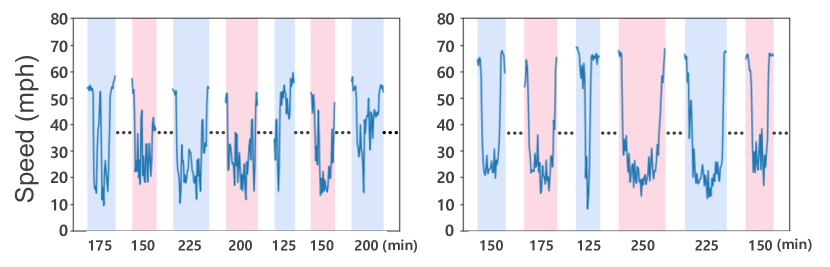
Figure 3. Two examples of the intervals extracted by ruptures with the y-axis showing the speed and the x-axis showing the duration for each interval.

Table 1 and Table 2 show the experimental results of both datasets, where we observe that ST-GRAT achieves state-of-the-art performance in the average scores. In particular, ST-GRAT excels at predicting speed after 15 and 30 minutes. ST-GRAT shows higher accuracy than GaAN, which is based on undirected spatial attention but neglects the proximity information. ST-GRAT also achieves higher performances compared to DCRNN and GraphWavenet, demonstrating that our spatial and temporal attention mechanism is more effective than that of the two models for predicting short-term future sequences.

We further evaluate ST-GRAT from several perspectives. First, we compare the forecasting performance of the models in separate time ranges. We do this because traffic congestion patterns in a city change dynamically over time. For example, some roads around residential areas are congested during regular rush hour periods, while those around industrial complexes are congested from late night to early morning (Lee et al., 2019). Table 3 shows the experimental results for four time ranges (00:00–05:59, 06:00–11:59, 12:00–17:59, and 18:00–23:59) and we find that ST-GRAT performs better than Graph WaveNet.

Secondly, to evaluate how ST-GRAT adapts to speed changes during rush hour times, we extract intervals of speeds from the data where road speeds change rapidly. We use “ruptures” (Truong et al., 2018), an algorithm for computing changing points in a non-stationary signal. Hyper-parameters of ruptures are 10, 1, and 6 for penalty value, jump, and minimum size, respectively. Fig. 3 shows the extracted intervals of two example roads where the y-axis represents speed and the x-axis represents the sequence of intervals. To find the intervals related to traffic congestion, we filter out intervals in which the slowest speeds are slower than 20 mph. Table 3 shows the performance comparison between ST-GRAT, Graph WaveNet and DCRNN, and we observe that our model captures the temporal dynamics of speed better than the others.

Third, we visualize the traffic speed of each model on line charts to illustrates the traffic speed prediction patterns during impeded time intervals in the METR-LA dataset. There is no time lag between ground truth and ST-GRAT prediction, while prediction traffic speed of other baseline models follow ground truth after reduced traffic speed as shown in Figure 4 (A). The ST-GRAT is more accurate with the abruptly changes and impeded interval than baseline models as shown in Figure 4 (B). This is because ST-GRAT exploits the overall graph structure information and effectively encodes temporal dynamics.

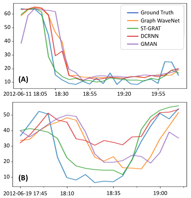
Figure 4. Traffic speed prediction visualization in the impeded intervals. ST-GRAT generates more accurate prediction and is robustness, especially when speeds abruptly change.

Table 3. Experimental results with different time ranges and intervals.

Model / T	15 min			30 min			1 hour			Average
	MAE	RMSE	MAPE	MAE	RMSE	MAPE	MAE	RMSE	MAPE	MAE	RMSE	MAPE
Our Model (00-06)	2.37	3.57	4.30%	2.41	3.67	4.44%	2.45	3.77	4.53%	2.38	3.63	4.37%
Graph WaveNet (00-06)	2.41	3.57	4.38%	2.45	3.68	4.50%	2.52	3.75	4.61%	2.44	3.65	4.47%
DCRNN (00-06)	2.4	3.58	4.36%	2.44	3.72	4.52%	2.48	3.8	4.6%	2.43	3.68	4.47%
GMAN (00-06)	2.39	3.59	4.35%	2.41	3.69	4.43%	2.43	3.75	4.48%	2.40	3.66	4.40%
Our Model (06-12)	2.55	5.31	6.93%	3.07	6.72	8.82%	3.68	8.16	10.93%	3.01	6.51	8.63%
Graph WaveNet (06-12)	2.67	5.43	7.55%	3.19	6.79	9.42%	3.73	8.01	11.28%	3.11	6.55	9.15%
DCRNN (06-12)	2.74	5.67	7.59%	3.28	7.16	9.6%	3.9	8.64	11.68%	3.22	6.95	9.35%
GMAN (06-12)	2.79	5.84	7.78%	3.22	7.00	9.27%	3.69	8.16	10.82%	3.17	6.83	9.09%
Our Model (12-18)	3.14	6.16	9.34%	3.80	7.69	12.02%	4.55	9.29	15.53%	3.72	7.47	11.88%
Graph WaveNet (12-18)	3.29	6.23	10.25%	3.80	7.49	12.41%	4.48	8.85	15.39%	3.77	7.31	12.28%
DCRNN (12-18)	3.33	6.43	10.11%	3.95	7.83	12.58%	4.66	9.33	15.66%	3.80	7.64	12.39%
GMAN (12-18)	3.48	6.87	10.78%	3.96	7.99	12.78%	4.48	9.12	15.26%	3.90	7.81	12.65%
Our Model (18-24)	2.34	4.77	5.69%	2.72	5.86	7.00%	3.21	7.10	8.60%	2.69	5.75	6.91%
Graph WaveNet (18-24)	2.41	4.83	6.09%	2.78	5.87	7.47%	3.19	6.90	8.99%	2.73	5.71	7.33%
DCRNN (18-24)	2.48	5.09	6.24%	2.85	6.19	7.79%	3.27	7.33	9.53%	2.81	6.04	7.66%
GMAN (18-24)	2.52	5.23	6.49%	2.82	6.16	7.78%	3.14	7.07	9.10%	2.78	6.03	7.65%
Our Model (Impeded Interval)	5.82	9.97	29.0%	7.94	13.31	41.20%	10.56	16.92	57.96%	7.81	13.32	41.04%
Graph WaveNet (Impeded Interval)	6.45	10.69	33.19%	8.62	14.10	45.89%	11.14	17.65	62.79%	8.44	14.05	45.49%
DCRNN (Impeded Interval)	6.44	10.41	33.75%	8.39	13.52	45.22%	10.71	16.76	60.93%	8.22	13.45	44.91%
GMAN (Impeded Interval)	6.94	11.55	36.05%	8.76	14.41	46.93%	10.74	17.22	60.38%	8.60	14.29	46.53%

Table 4. Ablation study of ST-GRAT with the METR-LA validation set.

	$L$	$d_{model}$	Embedding	$H$	Range	Directed	Prior	Sentinel	MAE
Our model	4	128	Distance	4	2	✔	✔	✔	2.80
(A)	2								3.02
	3								2.98
(B)		64							2.89
(C)			–						2.97
			Random						2.90
(D)				2					3.01
				8					2.88
(E)					1				2.98
(F)						–			2.87
(G)							–		2.85
(H)								–	2.89

4.3. Ablation Study

We conduct an ablation study to understand the impact of different hyper-parameters. Table 4 shows the experimental results where ${L}$, $d_{model}$, and ${H}$ denote the number of layers, dimension of hidden state features, and number of heads, respectively. “Embedding” and “Range” indicate different embedding methods and attention step sizes. If the range is one, it means that the model only attends nodes within a single step, such as directly connected nodes. If the range is two, it means the model attends nodes within two steps (i.e., directly linked nodes and their neighbors). The hyphens denote excluded parameters. “Directed” indicates that the input graph is a directed graph. Finally, “Prior” and “Sentinel” indicate whether the model uses a diffusion prior and sentinel vector or not. We show the average MAE prediction results from five-mins to one-hour measured by each evaluation metric. Other settings are identical to those used in subsection 4.1.

According to row (A), we observe that the number of layers proportionally affects the performance of our model. A deep model has better performance than a shallow model, because having a small number of layers causes the model to underfit. In row (B), we find that the dimension of the hidden vector also impacts the final performance. When the dimension of the hidden state vector increases, the key and query dimension also increases, allowing more information to be encoded. This motivates the model to better consider the elaborate relation between the query and key, leading to higher performance than a model with a small dimension of hidden vectors. Moreover, as we expected, we observe a positive correlation between the number of heads and the performance of the model in row (D). This is because as the number of heads increases, the model can capture more diverse aspects of spatial dependency than a model with a small number of heads. For example, if the model only has two heads, the first head might only consider the nodes that are experiencing traffic congestion while the second head only focuses on nodes that have light traffic.

Row (C) shows the results of different node embedding settings in comparison to our model, which utilize the distance between nodes as the node-embedding. We remove or add the embedding layer with different strategies as random initialization. Since the removed embedding layer and random initialization embedding does not have proximity information, both embedding layer models improperly perform attention, failing to attend more on close nodes than other distant nodes. By comparing different embedding settings, we observe that proximity information is hardly influencing the performance of our model.

From row (E), we show that the performance is also affected by the range of neighbor nodes that carry out the spatial attention process. The performance of $Range=2$ is better than that of $Range=1$ because the model with $Range=2$ considers more neighbor nodes than the model with $Range=1$. However, as the number of $Range$ increases, the computation cost of nodes (i.e., scaled-dot product operation) also increases.

Row (F) shows the effect of directed attention (inflow and outflow attention). In undirected attention, the spatial attention needs to compare the similarity of the query and key to all in-coming or out-going nodes from a particular node. As a result, even though undirected attention takes more nodes into consideration, its performance is lower than our model which uses directed attention. This experiment shows that our directed attention, which splits the heads into inflow and outflow, is suitable to solve traffic problems. Row (G) indicates whether the model applies the diffusion prior. The base model performance is better than the model that does not apply the diffusion prior. This is because the model adjusts the attention logits by utilizing a diffusion prior.

Row (H) shows the effect of a sentinel key-value vector, which is described in the spatial attention section. We find that the model that uses the sentinel vectors is better than the model that does not use sentinel vectors. This result indicates that the sentinel vectors help the model to improve robustness in the traffic prediction by avoiding unnecessary attentions.

5. Qualitative Analysis

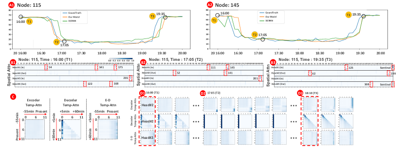
Figure 5. (A) Two line charts of the current node and neighbor node, (B) Spatial-attention heatmaps in different time steps, and (C) Temporal-attention heatmaps in different time steps at METR-LA dataset in impeded interval (2012/06/20 16:05–2012/06/20 20:10).

In this section, we describe how ST-GRAT captures spatio-temporal dependencies within a road network. Fig. 5 (A1) shows speed changes of Node 115, where the x- and y-axes represent time and speed (mph), respectively. As shown in Fig. 5 (A1), this road was congested from 16:50 and congestion was alleviated at approximately 19:35 (i.e., a typical congestion pattern in the evenings). The heatmaps of Fig. 5 (B1–B3) provide information on spatial attention of the last layer at different times (B1–T1, B2–T2, B3–T3). The y-axis at each head (in-out-in-out degrees) represents 12 time sequences, and the x-axis indicates the 207 nodes and the sentinel vector (last column).

First, we find that ST-GRAT gave more attention to six nodes (54, 122, 141, 168, 175, and 201) than others in light traffic (T1 in Fig. 5 (A1)). Then, as time passes from T1 to T2, Nodes 54 and 175 gradually received less attention, and Nodes 52, 111, 145, and 201 gained more attention, as shown in Fig. 5(B2). A notable observation is that ST-GRAT attended to Node 145 and Node 201 (i.e., dark blue bars) more than other nodes. We review speed records of Node 145 (Fig. 5, A2) due to its strong attention and find that the speed of Node 145 tended to precede that of Node 115 by about 30 minutes (Fig. 5 (A2)). In checking the correlations between pairs of nodes based on the VAR, we find that the speed pattern of Node 115 was highly correlated with that of Nodes 145 and 201 (0.59 and 0.56, respectively), while it was less correlated with other nodes (e.g., 0.48 with Node 52). An interesting point here is that the distances from the two nodes to Node 115 are different (0.9 miles from Node 145 and 7.64 miles from Node 201). This result shows that ST-GRAT learned dynamically changing spatial dependencies along with the graph structure information such as correlations and distances.

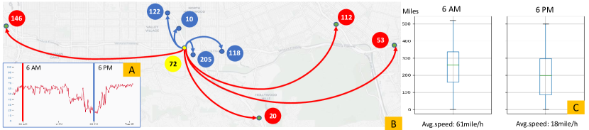
Figure 6. An example spatio-temporal dependency modeling based on node speeds and distance between query and key nodes. (A) Node 72’s speed trend; (B) nodes attended by Node 72 (yellow). Red and blue nodes are attended at 6am (unimpeded) and 6pm (impeded), respectively; and (C) an overall distribution of distances between the query nodes and corresponding key nodes. Node 72 attended the nodes closed to itself as the road became congested (p-value: $\ll 0.01$).

When the traffic congestion was alleviated at 19:35 (Fig. 5, T3), ST-GRAT attended to its sentinel vector of Head#1 (In) and Head#4 (Out), as shown in Fig. 5 (B3). This implies that ST-GRAT decided to utilize the existing features extracted from 18:45 to 19:05 by attending sentinel vector. ST-GRAT also attended to Node 125 (correlation: 0.43) for updating spatial dependency from a neighboring road (2.7 miles away from Node 115). We see a similar behavior in Head#4 (Out)–ST-GRAT focused on the sentinel vector, while attending to a distant Node 168 (correlation: 0.59, 7.8 miles away from Node 115). In the spatial attention, ST-GRAT dynamically uses new features from spatially correlated nodes or preserves existing features.

Next, we analyze the second head of the first layer in the encoder, decoder, and encoder-decoder (E-D) temporal attention (Fig. 5 (D1)). Note that Fig. 5(C) shows how the input and output sequences are mapped with each axis of the attention heatmaps in D1–D3. We see from Fig. 5 D1 that when Node 115 was not congested (T1), the temporal attention of the encoder and the decoder were equally spread out across all time steps. However, it is interesting that the temporal attention of the encoder gradually became divided into two regions (top-left and bottom-right) as the road became congested, as shown in a series of the heatmaps in Fig. 5 (D2). Here, the top-left region represents the information of past unimpeded conditions, while the other region contains information on the current impeded conditions. We believe this divided attention is reasonable, as ST-GRAT needed to consider two possible future directions at the same time–one with static congestion and another with a changing condition, possibly with a recovering speed. It is notable that the first column of the temporal attention of the decoder became darker (D2), which implies that ST-GRAT attended to recent information in the impeded condition. Overall, ST-GRAT uses the attention module in an adaptive manner with evolving traffic conditions for effectively capturing the temporal dynamics of traffic.

5.1. Attention Patterns in Different Traffic Conditions

In order to accurately model the spatial dependencies among roads, models need to dynamically adjust spatial correlations based on different traffic conditions (e.g., impeded condition) and the graph structure information, such as the connectivity, directions, and distances between nodes. However, previous models do not fully utilize the graph structure information in the spatial modeling (Zhang et al., 2018; Zheng et al., 2019). In cotrast, ST-GRAT incorporates graph structure features in the spatial attention by using diffusion priors and distance embedding and directed heads. In this section, we describe how ST-GRAT dynamically adjusts spatial correlations based on road conditions.

Fig. 6 describes an example attention pattern with Node 72. As shown in Fig. 6 (A), Node 72 is not congested early in 6 am (average speed: 61 miles/h), while it is impeded at 6 pm (average speed: 18 miles/h). Fig. 6 (B) shows that during the impeded traffic condition (6 pm), Node 72’s key nodes (blue dots) are much closer to the query Node 72 when compare to the unimpeded traffic condition (6 am) key nodes (red dots). Note that this is an magnified map, and key nodes with attention weights less than 0.1 are filtered out. Fig. 6 (C) shows the overall distance distribution of key nodes of 144 query nodes on June 4, 2012, 6 am and 6 pm. We choose the 144 query nodes that have less than 30 miles/h at the time and pick the longest distance between query and key nodes. We find that query nodes use the information of key nodes at significantly closer distances (average distance: 326.4 miles, STD: 206.7) in the impeded condition, compared to the unimpeded condition(average distance: 414.3, std: 186,3), according to the independent two sample t-test result (t[143]=3.3, p-value$<$0.01). This result shows that ST-GRAT predicts road speeds by considering the road speeds, distances between query and key nodes, and the road network, which leads to a better prediction performance than the existing models.

5.2. Analysis of Sentinel Vectors

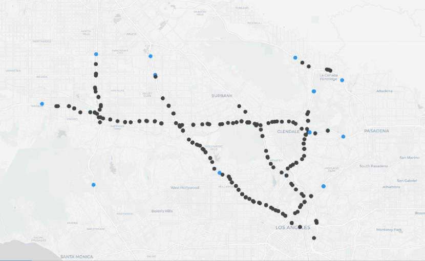
Figure 7. Highly affected nodes by sentinel vectors in METR-LA data. We visualize a sensor distribution of METR-LA dataset. Especially, we mark highly affected nodes by sentinel vector as blue color where sentinel attention weight($\alpha_{i,s}$) of the blue node has more than $0.35$.

To analyze how sentinel vectors work in the speed prediction tasks, we investigate the nodes that extensively utilize the vectors. For this, we first choose the nodes that have a sentinel attention weight ($\alpha_{i,s}$) higher than 0.35 (the upper 10% of the entire nodes), as shown in Fig. 7 as blue nodes. We then find it interesting that the nodes with high sentinel weights tend to be locate on the outskirts of the city. We also observe that they do not have many neighbor nodes compared to those in other areas (e.g., at the center of the city). Thus they do not have a sufficient pool of nodes with high spatial correlations for speed prediction. This means if a model is forced to encode new information based on spatial encoding, it is highly possible that it uses information of few other nodes, which may not be helpful for prediction. We also think that this attention strategy could negatively affect the performance of neighbor nodes that use this node as a key node.

To avoid such situations, ST-GRAT utilizes the sentinel vectors that contain features acquired in previous steps. To measure the effects of the vectors in such nodes, we compare ST-GRAT to its version without the sentinel vectors (ST-GRAT-NoSentinelVector) and find that ST-GRAT shows higher performance on the METR-LA test data (ST-GRAT: 2.27, ST-GRAT-NoSentinelVector: 2.34). As such, we believe that ST-GRAT improves the prediction performance by leveraging the sentinel vectors.

Table 5. The computation times on the METR-LA dataset.

Computation Time	DCRNN	GaAN	Graph Wavenet	GMAN	ST-GRAT
Training (s/epoch)	504.4	1461.4	203.89	552.1	341.7
Inference (s)	34.0	131.10	8.42	50.02	48.67

5.3. Computation Time

In this section, we report the computation costs of the models with the METR-LA dataset, as shown in Table 5. In terms of the training time, we find that ST-GRAT is faster ($O(1)$) than RNN-based models, such as DCRNN and GaAN which have $O(N)$ time complexity (Vaswani et al., 2017). Comparing ST-GRAT to the attention models, we find ST-GRAT is about four and three times faster than GaAN in the training and inference stages, respectively. ST-GRAT is also faster that GMAN which needs to consider more roads, as it does not uses the connectivity information between nodes. The Graph WaveNet performs best because it is a non-autoregressive model. Overall, ST-GRAT is the second best model in terms of the training time cost, and shows an average performance in terms of the inference time. However, ST-GRAT is more robust than other models in the impeded conditions (Table 3), which are more difficult to predict. Also, ST-GRAT provides interpretability (Fig. 5), which is an additional advantage over previous black-box models, such as GCNN-based models.

6. Conclusions

In this work, we presented ST-GRAT with a novel spatial and temporal attention for accurate traffic speed prediction. Spatial attention captures the spatial correlation among roads, utilizing graph structure information, while temporal attention captures the temporal dynamics of the road network by directly attending to features in long sequences. ST-GRAT achieves the state-of-the-art performance compared to existing methods on the METR-LA and the PEMS-BAY datasets, especially when speeds dynamically change in the short-term forecasting. Lastly, we visualize when and where ST-GRAT attends when making predictions during traffic congestion. As future work, we plan to conduct further experiments using ST-GRAT with different spatio-temporal domains and datasets, such as air quality data.

References

- (1)
- Atwood and Towsley (2016) James Atwood and Donald F. Towsley. 2016. Diffusion-Convolutional Neural Networks. In Proc. the Advances in Neural Information Processing Systems (NIPS).
- Ba et al. (2016) Jimmy Ba, Ryan Kiros, and Geoffrey E. Hinton. 2016. Layer Normalization. abs/1607.06450 (2016).
- Bengio et al. (2015) Samy Bengio, Oriol Vinyals, Navdeep Jaitly, and Noam Shazeer. 2015. Scheduled sampling for sequence prediction with recurrent neural networks. In Proc. the Advances in Neural Information Processing Systems (NIPS).
- Cho et al. (2014) Kyunghyun Cho, Dzmitry Bahdanau, Farhadi, and Yoshua Bengio. 2014. Neural Machine Translation by Jointly Learning to Align and Translate. Proc. the International Conference on Learning Representations (ICLR) (2014).
- Devlin et al. (2019) Jacob Devlin, Ming-Wei Chang, Kenton Lee, and Kristina Toutanova. 2019. BERT: Pre-training of Deep Bidirectional Transformers for Language Understanding. In Proc. the Annual Meeting of the Association for Computational Linguistics (ACL).
- Glorot and Bengio (2010) Xavier Glorot and Yoshua Bengio. 2010. Understanding the difficulty of training deep feedforward neural networks. In Proceedings of the Thirteenth International Conference on Artificial Intelligence and Statistics (Proceedings of Machine Learning Research), Vol. 9. PMLR, 249–256.
- Hendrycks and Gimpel (2016) Dan Hendrycks and Kevin Gimpel. 2016. Gaussian Error Linear Units (GELUs). arXiv:1606.08415 (2016).
- Hochreiter and Schmidhuber (1997) Sepp Hochreiter and Jürgen Schmidhuber. 1997. Long short-term memory. Neural computation 9, 8 (1997), 1735–1780.
- Kipf and Welling (2016) Thomas N Kipf and Max Welling. 2016. Semi-Supervised Classification with Graph Convolutional Networks. Proc. the International Conference on Learning Representations (ICLR) (2016).
- Lee et al. (2019) Chunggi Lee, Yeonjun Kim, Seungmin Jin, Dongmin Kim, Ross Maciejewski, David Ebert, and Sungahn Ko. 2019. A Visual Analytics System for Exploring, Monitoring, and Forecasting Road Traffic Congestion. IEEE Transactions on Visualization and Computer (2019).
- Li et al. (2018) Yaguang Li, Rose Yu, Cyrus Shahabi, and Yan Liu. 2018. Diffusion Convolutional Recurrent Neural Network: Data-Driven Traffic Forecasting. Proc. International Conference on Learning Representations (ICLR).
- Lin et al. (2017) Zhouhan Lin, Minwei Feng, Cicero Nogueira dos Santos, Mo Yu, Bing Xiang, Bowen Zhou, and Yoshua Bengio. 2017. A structured self-attentive sentence embedding. Proc. International Conference on Learning Representations (ICLR) (2017).
- Lu et al. (2016) Jiasen Lu, Caiming Xiong, Devi Parikh, and Richard Socher. 2016. Knowing When to Look: Adaptive Attention via a Visual Sentinel for Image Captioning. Proc. the IEEE conference on computer vision and pattern recognition(CVPR) (2016).
- Merity et al. (2017) Stephen Merity, Caiming Xiong, James Bradbury, and Richard Socher. 2017. Pointer Sentinel Mixture Models. Proc. the International Conference on Learning Representations (ICLR) (2017).
- Pan et al. (2018) Zheyi Pan, Yuxuan Liang, Junbo Zhang, Xiuwen Yi, Yingrui Yu, and Yu Zheng. 2018. HyperST-Net: Hypernetworks for Spatio-Temporal Forecasting. Proc. the Association for the Advancement of Artificial ntelligence (AAAI) (2018).
- Radford et al. (2019) Alec Radford, Jeff Wu, Rewon Child, David Luan, Dario Amodei, and Ilya Sutskever. 2019. Language Models are Unsupervised Multitask Learners. OpenAI Blog (2019).
- Seo et al. (2016) Minjoon Seo, Aniruddha Kembhavi, Ali Farhadi, and Hannaneh Hajishirzi. 2016. Bidirectional attention flow for machine comprehension. Proc. the International Conference on Learning Representations (ICLR) (2016).
- Srivastava et al. (2014) Nitish Srivastava, Geoffrey Hinton, Alex Krizhevsky, Ilya Sutskever, and Ruslan Salakhutdinov. 2014. Dropout: A Simple Way to Prevent Neural Networks from Overfitting. Journal of Machine Learning Research (JMLR) (2014).
- Tang et al. (2015) Jian Tang, Meng Qu, Mingzhe Wang, Ming Zhang, Jun Yan, and Qiaozhu Mei. 2015. Line: Large-scale information network embedding. In Proc. the International Conference on World Wide Web (WWW). 1067–1077.
- Truong et al. (2018) Charles Truong, Laurent Oudre, and Nicolas Vayatis. 2018. ruptures: change point detection in Python. arXiv preprint arXiv:1801.00826 (2018).
- van den Oord et al. ([n.d.]) Aäron van den Oord, Sander Dieleman, Heiga Zen, Karen Simonyan, Oriol Vinyals, Alex Graves, Nal Kalchbrenner, Andrew Senior, and Koray Kavukcuoglu. [n.d.]. WaveNet: A Generative Model for Raw Audio. In 9th ISCA Speech Synthesis Workshop. 125–125.
- Vaswani et al. (2017) Ashish Vaswani, Noam Shazeer, Niki Parmar, Jakob Uszkoreit, Llion Jones, Aidan N. Gomez, Lukasz Kaiser, and Illia Polosukhin. 2017. Attention Is All You Need. In Proc. the Advances in Neural Information Processing Systems (NIPS).
- Velickovic et al. (2018) Petar Velickovic, Guillem Cucurull, Arantxa Casanova, Adriana Romero, Pietro Lió, and Yoshua Bengio. 2018. Graph Attention Networks. Proc. International Conference on Learning Representations (ICLR) abs/1710.10903 (2018).
- Vlahogianni et al. (2014) Eleni I Vlahogianni, Matthew G Karlaftis, and John C Golias. 2014. Short-term traffic forecasting: Where we are and where we’re going. Transportation Research Part C: Emerging Technologies 43, Part 1 (2014), 3–19.
- Wu et al. (2019) Zonghan Wu, Shirui Pan, Guodong Long, Jing Jiang, and Chengqi Zhang. 2019. Graph WaveNet for Deep Spatial-Temporal Graph Modeling. In Proc. the International Joint Conference on Artificial Intelligence (IJCAI).
- Xu et al. (2015) Kelvin Xu, Jimmy Ba, Ryan Kiros, Kyunghyun Cho, Aaron C. Courville, Ruslan R. Salakhutdinov, Richard S. Zemel, and Yoshua Bengio. 2015. Show, Attend and Tell: Neural Image Caption Generation with Visual Attention. In Proc. the International Conference on Machine Learning (ICML).
- Yu et al. (2018) Bing Yu, Haoteng Yin, and Zhanxing Zhu. 2018. Spatio-temporal Graph Convolutional Networks: A Deep Learning Framework for Traffic Forecasting. In Proc. the International Joint Conference on Artificial Intelligence (IJCAI).
- Zhang et al. (2018) Jiani Zhang, Xingjian Shi, Junyuan Xie, Hao Ma, Irwin King, and Dit-Yan Yeung. 2018. GaAN: Gated Attention Networks for Learning on Large and Spatiotemporal Graphs. In Proc. the conference on uncertainty in artificial intelligence (UAI).
- Zhao et al. (2017) Zheng Zhao, Weihai Chen, Xingming Wu, Peter CY Chen, and Jingmeng Liu. 2017. LSTM network: a deep learning approach for short-term traffic forecast. IET Intelligent Transport Systems 11, 2 (2017), 68–75.
- Zheng et al. (2019) Chuanpan Zheng, Xiaoliang Fan, Cheng Wang, and Jianzhong Qi. 2019. Gman: A graph multi-attention network for traffic prediction. Proc. the Association for the Advancement of Artificial ntelligence (AAAI) (2019).
- Zivot and Wang (2006) Eric Zivot and Jiahui Wang. 2006. Vector autoregressive models for multivariate time series. Modeling Financial Time Series with S-Plus® (2006).