The Color Dipole Picture and extracting the ratio of structure functions at small $x$

Abstract

We present a set of formulas to extract the ratio $F_{L}(x,Q^{2})/F_{2}(x,Q^{2})$ and $R(x,Q^{2})$ from the proton structure function parameterized in the next-to-next-to-leading order of the perturbative theory at low $x$ values. The behavior of these ratios are considered with respect to the power-law behavior of the proton structure function. The results are compared with experimental data and the color dipole model bounds. These ratios are in good agreement with the HERA data throughout the fixed value of the invariant mass. The behavior of these ratios controlled by the nonlinear corrections at low values of $Q^{2}$. These results and comparison with HERA data demonstrate that the suggested method for the ratio of structure functions can be applied in analyses of the LHeC and FCC-eh projects.

.1 1. Introduction

Deep inelastic scattering (DIS) can be described in terms of the imaginary part of forward Compton-scattering amplitude. The inclusive deep inelastic scattering measurements are of importance to understanding the substructure of proton. It is known that the dominate source for distribution functions is the gluon density at low values of the Bjorken variable $x$. At low values of $Q^{2}$ (i.e. $Q^{2}\ll M^{2}_{Z}$) the contribution of Z exchange is negligible. The reduced cross section in terms of the structure function $F_{2}$ and the longitudinal structure function $F_{L}$ is defined in the following form:

$${\sigma_{r}}(x,Q^{2}) = \frac{d^{2}\sigma}{dxdQ^{2}}.\frac{Q^{4}x}{2{\pi}\alpha^{2}Y_{+}}$$ (1)

$$=F_{2}(x,Q^{2})[1-\frac{y^{2}}{Y_{+}}\frac{F_{L}(x,Q^{2})}{F_{2}(x,Q^{2})}],$$

where $Y_{+}=1+(1-y)^{2}$ and $\alpha$ is the fine structure constant. The reduced cross section depends on the square $s$ of the center-of-mass energy and the inelasticity variable $y=Q^{2}/(xs)$ where $Q^{2}$ refers to the photon virtuality. At high values of $y$ a characteristic bending of the reduced cross section is observed. It is attributed to the contribution caused by the longitudinal structure function. The structure functions (i.e., $F_{2}$ and $F_{L}$) can be written in terms of the $\gamma^{*}p$ total cross section as

$$F_{2}(x,Q^{2}) = \frac{Q^{2}}{4\pi^{2}\alpha}[\sigma_{L}^{\gamma^{*}p}(x,Q^{2})+\sigma_{T}^{\gamma^{*}p}(x,Q^{2})],$$

$$\mathrm{and}~{}~{}~{}~{}~{}~{}~{}~{}~{}~{}~{}~{}~{}~{}~{}~{}~{}$$

$$F_{L}(x,Q^{2}) = \frac{Q^{2}}{4\pi^{2}\alpha}\sigma_{L}^{\gamma^{*}p}(x,Q^{2}),$$ (2)

where the subscript $L$ and $T$ refer to the transverse and longitudinal polarization state of the exchanged boson. The ratio of the longitudinal to transverse cross sections is termed

$$R(x,Q^{2})=\frac{\sigma_{L}(x,Q^{2})}{\sigma_{T}(x,Q^{2})}=\frac{F_{L}}{F_{2}-F_{L}}.$$ (3)

The longitudinal structure function is directly sensitive to the gluon density. Beyond the parton model the $F_{L}$ effects can be sizable, hence it can not be longer neglected. Also, the longitudinal structure function is predominant in cosmic neutrino-hadron cross section scattering. This behavior for the longitudinal structure function will check at the Large Hadron electron Collider (LHeC) project which runs to beyond a TeV in center-of-mass energy [1-3]. It is a high-energy lepton-proton and lepton-nucleus collider based at CERN. The LHeC center-of-mass energy is $\sqrt{s}\simeq 1.3~{}\mathrm{TeV}$ which it is about 30 times the center of mass energy range of ep collisions at hadron electron ring accelerator (HERA). The kinematics in the ($x,Q^{2}$) plane of the LHeC for electron and positron neutral-currents reaches $\simeq 1\mathrm{TeV}^{2}$ and $\simeq 10^{-6}$ for $Q^{2}$ and $x$ respectively.
The Future Circular Collider (FCC) programme is developing designs for a higher luminosity particle collider [3]. In this collider the FCC-eh with $50~{}\mathrm{TeV}$ proton beams colliding with 60 GeV electrons which the center-of-mass energy is $3.5~{}\mathrm{TeV}$. These colliders (i.e., LHeC and FCC-eh) lead into a region of high parton densities at small Bjorken $x$. Deep inelastic scattering measurements at FCC-eh and LHeC will allow the determination of the longitudinal structure function which its determination was so difficult at HERA.
We known that HERA have been combined the neutral current (NC) interaction data for $0.045\leq Q^{2}\leq 50,000~{}\mathrm{GeV}^{2}$ and $6\times 10^{-7}\leq x\leq 0.65$ at values of the inelasticity $0.005\leq y\leq 0.95$ [4]. The highest center-of-mass energy in deep inelastic scattering of electrons on protons was $\sqrt{s}\simeq 320~{}\mathrm{GeV}$. These data that collected from 1992 until 2015 are listed in Table I. The final measurement of $F_{L}$ at HERA was determined in Ref.[5]. HERA collected $ep$ collision data with the H1 detector at a electron beam energy of $27.6~{}\mathrm{GeV}$ and proton beam energies of $920,575$ and $460~{}\mathrm{GeV}$, which allowed a measurement of structure functions at $x$ values $6.5{\times}10^{-4}{\leq}x{\leq}0.65$ and $Q^{2}$ values $35~{}\mathrm{GeV}^{2}{\leq}Q^{2}{\leq}800~{}\mathrm{GeV}^{2}$. The variation in inelasticity $y$ was achieved at HERA by comparing high statistics data at highest energy, $E_{p}=920~{}\mathrm{GeV}$, with about $13\mathrm{pb}^{-1}$ of data at $460~{}\mathrm{GeV}$ and $7\mathrm{pb}^{-1}$ at $575~{}\mathrm{GeV}$.
This continues the path of deep inelastic scattering is the best tool to probe the ratio $F_{L}/F_{2}$ into unknown areas of physics at very low-$x$ values and new colliders kinematics. In this region, the gluon distribution has a nonlinear behavior. The nonlinear effects are provided by a multiple gluon interaction which lead to the nonlinear terms in the derivation of the linear DGLAP evolution equations. Therefore the standard linear DGLAP evolution equations have been modified by the nonlinear corrections. Indeed the origin of the shadowing correction, in pQCD interactions, is primarily considered as the gluon recombination ($g+g\rightarrow g$) which is simply the inverse process of gluon splitting ($g\rightarrow g+g$). Gribov, Levin, Ryskin, Mueller and Qiu (GLR-MQ) [6] performed a detailed study of these recombination processes. This widely known as the GLR-MQ equation and involves the two-gluon distribution per unit area of the hadron. This equation predicts a saturation behavior of the gluon distribution at very small $x$ [7-9]. A closer examination of the small $x$ scattering is resummation powers of $\alpha_{s}\ln(1/x)$ where leads to the $k_{T}$-factorization form [10]. In the $k_{T}$-factorization approach the large logarithms $\ln(1/x)$ are relevant for the unintegrated gluon density in a nonlinear equation. Solution of this equation develops a saturation scale where tame the gluon density behavior at low values of $x$ and this is an intrinsic characteristic of a dense gluon system.
The paper is organized as follows. In sect.2, we give a summary about the ratio of structure functions based on the color dipole picture. We will study the ratio $F_{L}/F_{2}$ with respect to the $F_{2}$ parameterization in section 3. Then we introduce a method to calculate the ratio $F_{L}/F_{2}$ applying the effective exponents behavior. In sect.4 we utilize obtained solution to calculate the nonlinear behavior of the ratio $F_{L}/F_{2}$ at hot-spot point. Section 5 contains the results and discussions. The behavior of the ratio $F_{L}/F_{2}$ and $R$ are compared with H1 data at fixed value of invariant mass in this section. Finally, we give our conclusions in sect.6.

.2 2. A Short Theoretical Input

In this section we briefly present the theoretical part of our analysis. The reader can be refereed to the Refs.[11-16] for more details. At low $x$ (i.e., $x\ll 1$ where $x\simeq\frac{Q^{2}}{W^{2}}$ and $W$ refers to the photon-proton center-of-mass energy), the virtual spacelike photon fluctuates on the proton are defined into on-shell quark-antiquark, $q\overline{q}$, vector state. In this process photon interact with the proton via coupling of two gluons to the $q\overline{q}$ color dipole. This formalism called the color-dipole picture (CDP) of low-$x$ DIS [11-13]. The mass of $q\overline{q}$ dipole, in terms of the transverse momentum $\overrightarrow{k_{\bot}}$ is realized by $M^{2}_{q\overline{q}}=\frac{\overrightarrow{k_{\bot}}^{2}}{z(1-z)}$. Here $\overrightarrow{k_{\bot}}$ define as to the photon direction and variable $z$, with $0\leq z\leq 1$, characterizes the distribution of the momenta between quark and antiquark. The lifetime of the $q\overline{q}$ dipole is defined by $\tau=\frac{W^{2}}{Q^{2}+M^{2}_{q\overline{q}}}\gg\frac{1}{M_{p}}$. This lifetime is much longer than interaction time with the target at small $x$. This condition not only restricts the kinematical range of the color dipole model to the region $x\ll 1$ but also saturate the $\gamma^{*}$-proton cross section with $x\leq 0.1$ [14-16].
In the dipole picture, the total deep inelastic cross-section can be factorized in the following form

$$\sigma_{L,T}^{\gamma^{*}p}(x,Q^{2}) = \int dzd^{2}\mathbf{r}_{\bot}|\Psi_{\gamma}^{L,T}(\mathbf{r}_{\bot},z(1-z),Q^{2})|^{2}$$ (4)

$${\times}\sigma_{q\overline{q}}(\mathbf{r}_{\bot},z(1-z),W^{2}),$$

where $\Psi_{\gamma}^{L,T}$ are the appropriate spin averaged light-cone wave functions of the photon and $\sigma_{q\overline{q}}(r,z,W^{2})$ is the dipole cross-section which it related to the imaginary part of the $(q\overline{q})p$ forward scattering amplitude. The square of the photon wave function describes the probability for the occurrence of a $(q\overline{q})$ fluctuation. Here the transverse size related to the photon polarization [13-16,17].
The ratio of structure functions is expressed in terms of the longitudinal-to-transverse ratio of the photo absorption cross sections. This ratio has been defined by

$$\frac{F_{L}(x,Q^{2})}{F_{2}(x,Q^{2})}=\frac{R(x,Q^{2})}{1+R(x,Q^{2})}.$$ (5)

In Refs.[11-15], authors show that at large $Q^{2}$ (i.e., $Q^{2}\gg\Lambda_{sat}^{2}(W^{2})$), the ratio of photo absorption cross sections is given by the theoretically preferred value of $\rho$ which

$$R(W^{2},Q^{2})|_{Q^{2}\gg\Lambda^{2}_{sat}(W^{2})} = \frac{1}{2\rho},$$

$$\mathrm{and}~{}~{}~{}\rho_{W}=\rho=\frac{4}{3}.$$ (6)

The structure function $F_{2}(x,Q^{2})$ has been defined by the color-dipole cross sections [11], as the leading contribution is given by the following form

$$F_{2}(x,Q^{2}) = \frac{Q^{2}}{4\pi^{2}\alpha}\sigma^{\gamma^{*}p}(W^{2},Q^{2})=\frac{Q^{2}}{4\pi^{2}\alpha}(\sigma_{L}^{\gamma^{*}p}(W^{2},Q^{2})$$ (7)

$$+\sigma_{T}^{\gamma^{*}p}(W^{2},Q^{2})),$$

which at large-$Q^{2}$ limit, the equation becomes [12]

$$F_{2}(x,Q^{2}) = \frac{R_{e^{+}e^{-}}}{36\pi^{2}}(T(W^{2})+\frac{1}{2}L(W^{2})),$$ (8)

where $R_{e^{+}e^{-}}=10/3$ for even active flavor number.
In Refs.[11, 12] as to some assumptions about the sea-quark and gluon distribution behavior into the kinematic variable $W^{2}$ one obtained that

$$T(W^{2})=\rho L(W^{2}).$$ (9)

The structure function $F_{2}$ in (8) has been defined by

$$F_{2}(x,Q^{2}) = \frac{R_{e^{+}e^{-}}}{36\pi^{2}}T(W^{2})(1+\frac{1}{2\rho}).$$ (10)

Indeed the longitudinal-to-transverse ratio of the photoabsorbtion cross sections related to $\rho\equiv\rho(x,Q^{2})$ as

$$R(x,Q^{2})=\frac{\sigma_{L}^{\gamma^{*}p}(W^{2},Q^{2})}{\sigma_{T}^{\gamma^{*}p}(W^{2},Q^{2})}=\frac{1}{2\rho(x,Q^{2})}.$$ (11)

The ratio $F_{L}/F_{2}$ is expressed in terms of $\rho$ as we have it:

$$\frac{F_{L}(x,Q^{2})}{F_{2}(x,Q^{2})}=\frac{1}{1+2\rho(x,Q^{2})}.$$ (12)

Factor $2$ originates from the difference between the transverse and longitudinal photon wave function. Also factor $\rho$ is associated with different interaction of photons into $q\overline{q}$ pairs, $\gamma^{*}_{L,T}\rightarrow q\overline{q}$. The value of $\rho$ predicted to be $1$ in Ref.[11] or $\frac{4}{3}$ in Refs.[12, 13]. A similar relation based on the fit to the experimental data around $\rho=1$ was found in Ref.[11] in the form

$$\overline{\sigma}_{(q\overline{q})_{T}^{J=1}}(\overrightarrow{l}_{\bot}^{\prime 2},W^{2})=\overline{\sigma}_{(q\overline{q})_{L}^{J=1}}(\overrightarrow{l}_{\bot}^{\prime 2},W^{2}),$$ (13)

where they are related to the color-dipole cross sections concerning the gauge-theory structure as

$${\sigma}_{(q\overline{q})_{p}}(\overrightarrow{r}_{\bot},W^{2}) = \int d^{2}{l}_{\bot}\overline{\sigma}_{(q\overline{q})_{p}}(\overrightarrow{l}_{\bot}^{2},W^{2})$$ (14)

$$\times(1-e^{-i\overrightarrow{l}_{\bot}\overrightarrow{r}_{\bot}}).$$

For the specific value $\rho=1$ (i.e., helicity independent) the ratio of cross sections $R(W^{2},Q^{2})$ is found to be $R(W^{2},Q^{2})=0.5$. Therefore the ratio of structure functions was obtained to be $F_{L}(W^{2},Q^{2})/F_{2}(W^{2},Q^{2})=1/3=0.333$.
In Refs.[12, 13] the relation between the $q\overline{q}$-proton interactions (i.e., Eq.13) was derived by a proportionality factor $\rho$,

$$\overline{\sigma}_{(q\overline{q})_{T}^{J=1}}(\overrightarrow{l}_{\bot}^{\prime 2},W^{2})=\rho\overline{\sigma}_{(q\overline{q})_{L}^{J=1}}(\overrightarrow{l}_{\bot}^{\prime 2},W^{2}),$$ (15)

where $\rho=\frac{<\overrightarrow{k}^{2}_{\bot}>_{L}}{<\overrightarrow{k}^{2}_{\bot}>_{T}}$. The average transverse momenta squared with respect to the longitudinal and transverse photons is defined by the following forms

$$<\overrightarrow{k}^{2}_{\bot}>_{L,T}=M_{q\overline{q}}^{2}\int_{0}^{1}dzz(1-z)f_{L,T}(z),$$ (16)

where

$$f_{L}(z)=6z(1-z)$$ (17)

and

$$f_{T}(z)=\frac{3}{2}(1-2z(1-z)).$$ (18)

Then the factor $\rho$ corresponds to

$$\rho=\frac{<\overrightarrow{k}^{2}_{\bot}>_{L}}{<\overrightarrow{k}^{2}_{\bot}>_{T}}=\frac{4}{3},$$ (19)

which shows $R(W^{2},Q^{2})=3/8=0.375$ and the ratio of structure functions is proportional to $F_{L}(W^{2},Q^{2})/F_{2}(W^{2},Q^{2})=3/11=0.273$ [12, 13]. Some analytical solutions [18, 19] have been shown that in the dipole model there is a strict bound for the ratio of structure functions as $\frac{F_{L}(x,Q^{2})}{F_{2}(x,Q^{2})}<0.27$. In realistic dipole-proton cross section authors in Ref.[20] have been discussed that the bound is lower than $0.27$ with the ratio $\simeq 0.22$. In Ref.[21] the ratio $R$ is found at $R=0.260{\pm}0.050$ which this value is constant at the region $7.10^{-5}<x<2.10^{-3}$ and $3.5\leq Q^{2}\leq 45~{}\mathrm{GeV^{2}}$. In color dipole model the ratio $R$ leads to the bound $R\leq 0.372$ [19, 22]. In Ref.[23] ZEUS collaboration is shown that the overall value of $R$ from both the unconstrained and constrained fits is $R=0.105^{+0.055}_{-0.037}$ in a wide range of $Q^{2}$ values ($5\leq Q^{2}\leq 110~{}GeV^{2}$). These results are correspondent to the helicity fluctuations of the photon on the proton. Our insight into the dynamics of these fluctuations might determined $\rho(x,Q^{2})$ in comparison with the measurement data and provides some constraints on the CDP bounds.

.3 3. Formalism

In perturbative QCD, the longitudinal structure function in terms of the coefficient functions at small $x$ is given by

$$x^{-1}F_{L}=<e^{2}>(C_{L,q}{\otimes}q_{s}+C_{L,g}{\otimes}g).$$ (20)

Here $<e^{k}>$ is the average of the charge $e^{k}$ for the active quark flavors, $<e^{k}>=n_{f}^{-1}\sum_{i=1}^{n_{f}}e_{i}^{k}$. The perturbative expansion of the coefficient functions can be written as [24]

$$C_{L,a}(\alpha_{s},x)=\sum_{n=1}a(t)^{n}c_{L,a}^{n}(x),$$ (21)

where $n$ is the order in the running coupling constant. The running coupling constant in the high-loop corrections of the above equation is expressed entirely thorough the variable $a(t)$, as $a(t)=\frac{\alpha_{s}}{4\pi}$. The explicit expression for the coefficient functions in LO up to NNLO are presented in Refs.[25, 26].
At small $x$ the linear DGLAP $Q^{2}$ evolution equations [27] related to the BFKL [28] type of law. In this theoretical framework, the gluon density is expressed in terms of the structure functions, $F_{2}$ and $F_{L}$, which it is a test higher order QCD at small $x$. In this respect, several equations have been proposed to define the gluon density by the $F_{2}$ scaling violation. In Refs.[29, 30] a similar relation based on the $F_{2}$ and derivative of $F_{2}$ related to the pomeron behavior was suggested with the result

$$G(x,Q^{2}) = \frac{1}{\Theta_{qg}(x,Q^{2})}[\frac{{\partial}F_{2}(x,Q^{2})}{{\partial}{\ln}Q^{2}}$$ (22)

$$-\Phi_{qq}(x,Q^{2})F_{2}(x,Q^{2})].$$

The kernels for the quark and gluon sectors (denoted by $\Phi$ and $\Theta$) presented by the following forms

$$\Theta_{qg}(x,Q^{2}) = P_{qg}(x,\alpha_{s})\otimes x^{\lambda_{g}},$$

$$\Phi_{qq}(x,Q^{2}) = P_{qq}(x,\alpha_{s})\otimes x^{\lambda_{s}}.$$ (23)

The one, two- and three-loop splitting functions (LO, NLO and NNLO) for the parton distributions have been shown in Ref.[31]. The exponents $\lambda_{s}$ and $\lambda_{g}$ are defined by the derivatives of the distribution functions by the following forms as $\lambda_{s}={\partial\ln F_{2}^{s}(x,Q^{2})}/{\partial\ln(1/x)}$ and $\lambda_{g}={\partial\ln G(x,Q^{2})}/{\partial\ln(1/x)}$. The running coupling constant $\alpha_{s}$ has the following form in NNLO analysis

$$\alpha_{s}^{\rm NNLO} = \frac{4\pi}{\beta_{0}t}[1-\frac{\beta_{1}{\ln}t}{\beta_{0}^{2}t}+\frac{1}{(\beta_{0}t)^{2}}[(\frac{\beta_{1}}{\beta_{0}})^{2}$$ (24)

$$(\ln^{2}t-{\ln}t+1)+\frac{\beta_{2}}{\beta_{0}}]],$$

where $\beta_{0}=\frac{1}{3}(33-2n_{f})$, $\beta_{1}=102-\frac{38}{3}n_{f}$ and $\beta_{2}=\frac{2857}{6}-\frac{6673}{18}n_{f}+\frac{325}{54}n_{f}^{2}$. The variable $t$ is defined as $t={\ln}(\frac{Q^{2}}{\Lambda^{2}})$ and $\Lambda$ is the QCD cut- off parameter for each heavy quark mass threshold as we take the $n_{f}=4$ for $m_{c}^{2}<\mu^{2}<m^{2}_{b}$.
In what follows it is convenient to use a similar method was found in Ref.[32] for the longitudinal structure function as we have it:

$$F_{L}(x,Q^{2}) = F_{2}(x,Q^{2})I_{L,q}(x,Q^{2})$$ (25)

$$+G(x,Q^{2})I_{L,g}(x,Q^{2}),$$

where the analytical results for the compact form of the kernels are given in Appendix A.
With respect to Eq.22, one can rewrite the longitudinal structure function concerning the proton structure function $F_{2}(x,Q^{2})$ and its derivative $\partial F_{2}(x,Q^{2})/\partial{\ln}Q^{2}$, as we will have

$$F_{L}(x,Q^{2}) = \frac{I_{L,g}(x,Q^{2})}{\Theta_{qg}(x,Q^{2})}\frac{{\partial}F_{2}(x,Q^{2})}{{\partial}{\ln}Q^{2}}+\{I_{L,q}(x,Q^{2})$$ (26)

$$-\Phi_{qq}(x,Q^{2})\frac{I_{L,g}(x,Q^{2})}{\Theta_{qg}(x,Q^{2})}\}F_{2}(x,Q^{2}).$$

Therefore the ratio $F_{L}/F_{2}$ takes the form

$$\frac{F_{L}(x,Q^{2})}{F_{2}(x,Q^{2})}=\eta(x,Q^{2})+\zeta(x,Q^{2})\frac{{\partial}{\ln}F_{2}(x,Q^{2})}{{\partial}{\ln}Q^{2}},$$ (27)

where

$$\eta(x,Q^{2}) = I_{L,q}(x,Q^{2})-\Phi_{qq}(x,Q^{2})\frac{I_{L,g}(x,Q^{2})}{\Theta_{qg}(x,Q^{2})},$$

$$\zeta(x,Q^{2}) = \frac{I_{L,g}(x,Q^{2})}{\Theta_{qg}(x,Q^{2})}.$$ (28)

By means of these equations we have extracted the ratio of structure functions from the parameterization of $F_{2}$, using the slopes ${\partial}{\ln}F_{2}/{\partial}{\ln}Q^{2}$ proposed in Ref.[33].

3.1. The ratio of structure functions using the $F_{2}$ parameterization

Authors of Ref.[33] suggested a new parametrization which describes fairly good the available experimental data on the proton structure function in an agreement with the Froissart bound behavior. Also a theoretical analysis investigated the behavior of the longitudinal structure function at small $x$ by employing this behavior is studied in Ref.[34]. The explicit expression for the $F_{2}$ parametrization [33] is given by the following form

$$F^{\gamma p}_{2}(x,Q^{2}) = D(Q^{2})(1-x)^{n}\sum_{m=0}^{2}A_{m}(Q^{2})L^{m},$$ (29)

where

$$A_{0}(Q^{2}) = a_{00}+a_{01}{\ln}(1+\frac{Q^{2}}{\mu^{2}}),$$

$$A_{1}(Q^{2}) = a_{10}+a_{11}{\ln}(1+\frac{Q^{2}}{\mu^{2}})+a_{12}{\ln}^{2}(1+\frac{Q^{2}}{\mu^{2}}),$$

$$A_{2}(Q^{2}) = a_{20}+a_{21}{\ln}(1+\frac{Q^{2}}{\mu^{2}})+a_{22}{\ln}^{2}(1+\frac{Q^{2}}{\mu^{2}}),$$

$$D(Q^{2}) = \frac{Q^{2}(Q^{2}+\lambda M^{2})}{(Q^{2}+M^{2})^{2}},$$

$$L^{m} = \ln^{m}(\frac{1}{x}\frac{Q^{2}}{Q^{2}+\mu^{2}}).$$ (30)

Here $M$ and $\mu^{2}$ are the effective mass a scale factor respectively. The additional parameters with their statistical errors are given in Table II. Equation (29) obtained from a combined fit of the H1 and ZEUS collaborations data [35] in a range of the kinematical variables $x$ and $Q^{2}$( $x<0.01$ and $0.15<Q^{2}<3000~{}\mathrm{GeV}^{2}$).
Therefore with respect to the parameterization of $F_{2}$ the final result for the ratio $F_{L}/F_{2}$ is

$$\frac{F_{L}(x,Q^{2})}{F_{2}(x,Q^{2})} = \eta(x,Q^{2})+\zeta(x,Q^{2})\{\frac{{\partial}{\ln}D(Q^{2})}{{\partial}{\ln}Q^{2}}$$ (31)

$$+\frac{{\partial}{\ln}(\sum_{m=0}^{2}A_{m}(Q^{2})L^{m})}{{\partial}{\ln}Q^{2}}\}.$$

At last, the ratio of the longitudinal to transverse cross sections is expressed in terms of the $F_{2}$ parameterization as we have it:

$$R(x,Q^{2})=Eq.(31)/(1-Eq.(31)).$$ (32)

3.2. The ratio of structure functions using the exponents behavior

At small $x$ and sufficiently large $Q^{2}$, the deep inelastic scattering is recognized as elastic diffractive forward scattering of the photon fluctuations,$(q\overline{q})^{J=1}_{L,T}$, on the proton [11-15]. The proton structure function in CDP is given by the single variable $W^{2}$ as

$$F_{2}(x,Q^{2})=F_{2}(W^{2}=\frac{Q^{2}}{x}).$$ (33)

A power-law for the $W$-dependence of $F_{2}(W^{2})$ can be exploited in Eq.(33) as

$$F_{2}(W^{2})\sim(W^{2})^{\lambda_{s}}=(\frac{Q^{2}}{x})^{\lambda_{s}},$$ (34)

where the exponent $\lambda_{s}$ is defined by

$$\lambda_{s} = \frac{\partial\ln F_{2}(W^{2})}{\partial\ln W^{2}}.$$ (35)

Substitution of (35) into (27) we get

$$\frac{F_{L}(W^{2})}{F_{2}(W^{2})}=\eta(W^{2})+\zeta(W^{2})\lambda_{s}|_{x}.$$ (36)

Equivalently the ratio of structure functions, in terms of $\rho_{w}$, is obtained by the following form

$$\frac{1}{1+2\rho_{w}}=\eta(W^{2})+\zeta(W^{2})\lambda_{s},$$ (37)

where

$$\rho_{w}=\frac{1-\eta(W^{2})-\zeta(W^{2})\lambda_{s}}{2(\eta(W^{2})+\zeta(W^{2})\lambda_{s})},$$ (38)

or

$$R_{w}=\frac{\eta(W^{2})+\zeta(W^{2})\lambda_{s}}{1-\eta(W^{2})-\zeta(W^{2})\lambda_{s}}.$$ (39)

According to the Regge phenomenology, the density functions can be controlled by pomeron exchange at low $x$ since these behaviors for the singlet and gluon distributions are correspondent to the BFKL pomeron. The exponent for the gluon distribution is comparable with the so-called hard pomeron intercept. This behavior is defined with a value of $\lambda_{g}{\simeq}0.424$ which it is the hard pomeron part of Regge phenomenology [36]. We choice that the singlet exponent value is consistent with the experimental data and CDP bound if one definite value $0.27\leq\lambda_{s}\leq 0.33$ in a wide range of $Q^{2}$ values.
The strong rise into the $k_{T}$ factorization formula is also true for the singlet structure function. This behavior comes from resummation of large powers of $\alpha_{s}\ln 1/x$ where its achieved by the use of the $k_{T}$ factorization formalism. The small-$x$ resummation requires an all-order class of subleading corrections in order to lead to stable results [37]. However the singlet effective pomeron is $Q^{2}$-dependent when structure functions fitted to the experimental data at low values of $x$. Here, we take into account the effects of kinematics which lead to a shift from the pomeron exponent to the effective exponent for singlet structure function.
To better illustrate our calculations at all $Q^{2}$ values, we used the singlet effective exponent in the form of $\lambda^{s}(Q^{2})$. The singlet effective exponent is presented based on the H1 and H1-ZEUS combined data for the proton structure functions at $4<Q^{2}<200~{}GeV^{2}$. In Ref.[38], an eyeball fit was given by the following form

$$\lambda^{s}_{eff}(Q^{2})=0.13+0.1(\frac{Q^{2}}{10})^{0.35}.$$ (40)

Also authors in Ref.[39] have derived the phenomenological exponent of singlet density for combined HERA $e^{+}p$ DIS data [40] within the saturation model where $\lambda^{s}_{phn}(Q^{2})$ is assumed to be of the form

$$\lambda^{s}_{phn}(Q^{2})=0.329+0.1\log(\frac{Q^{2}}{90}).$$ (41)

.4 4. Nonlinear correction to the ratio $F_{L}/F_{2}$

The behavior of the singlet density will be checked at new colliders ( LHeC and FCC-eh) which runs to beyond a TeV in center-of-mass energy. Clearly, there would be an increase in the precision of parton density and in the low $x$ kinematic region in these colliders. So one should consider the low- $x$ behavior of the singlet distribution using the nonlinear GLR-MQ evolution equation. The shadowing correction to the evolution of the singlet quark distribution can be written as [41]

$$\frac{{\partial}xq(x,Q^{2})}{{\partial}{\ln}Q^{2}} = \frac{{\partial}xq(x,Q^{2})}{{\partial}{\ln}Q^{2}}|_{DGLAP}$$ (42)

$$-\frac{27\alpha_{s}^{2}}{160R^{2}Q^{2}}[xg(x,Q^{2})]^{2}.$$

Eq.(42) can be rewrite in a convenient form as

$$\frac{{\partial}F_{2}(x,Q^{2})}{{\partial}{\ln}Q^{2}}=\frac{{\partial}F_{2}(x,Q^{2})}{{\partial}lnQ^{2}}|_{DGLAP}-\frac{5}{18}\frac{27\alpha_{s}^{2}}{160R^{2}Q^{2}}$$

$${\times}[xg(x,Q^{2})]^{2}.$$ (43)

The first term is the standard DGLAP evolution equation and the value of $R$ is the correlation radius between two interacting gluons. It will be of the order of the proton radius $(R\simeq 5\hskip 2.84544ptGeV^{-1})$ if the gluons are distributed through the whole of proton, or much smaller $(R\simeq 2\hskip 2.84544ptGeV^{-1})$ if gluons are concentrated in hot- spot within the proton.
Combining Eqs. (22) and (43), one can consider the nonlinear correction to the gluon distribution function as we have

$$G(x,Q^{2}) = \frac{1}{\Theta_{qg}(x,Q^{2})}[\frac{{\partial}F_{2}(x,Q^{2})}{{\partial}{\ln}Q^{2}}-\frac{5}{18}\frac{27\alpha_{s}^{2}}{160R^{2}Q^{2}}{\times}$$

$$G^{2}(x,Q^{2})-\Phi_{qq}(x,Q^{2})F_{2}(x,Q^{2})].$$

Eq.(44) can be rewritten in the following form:

$$G(x,Q^{2})+\frac{1}{\Theta_{qg}(x,Q^{2})}\frac{5}{18}\frac{27\alpha_{s}^{2}}{160R^{2}Q^{2}}G^{2}(x,Q^{2})=$$

$$\frac{1}{\Theta_{qg}(x,Q^{2})}[\frac{{\partial}F_{2}(x,Q^{2})}{{\partial}{\ln}Q^{2}}-\Phi_{qq}(x,Q^{2})F_{2}(x,Q^{2})].$$ (45)

Equation (45) is a second-order equation related to the gluon distribution function which can be solved as

$$\mathcal{G}(x,Q^{2}) = G(x,Q^{2})[1-\frac{\mathcal{A}(x,Q^{2})}{\Theta_{qg}(x,Q^{2})}G(x,Q^{2})$$ (46)

$$+2(\frac{\mathcal{A}(x,Q^{2})}{\Theta_{qg}(x,Q^{2})}G(x,Q^{2}))^{2}$$

$$-5(\frac{\mathcal{A}(x,Q^{2})}{\Theta_{qg}(x,Q^{2})}G(x,Q^{2}))^{3}+....]$$

$$=G(x,Q^{2})[1-\mathcal{N}+2\mathcal{N}^{2}-5\mathcal{N}^{3}+....]$$

$$=G(x,Q^{2})[\mathcal{NLC}],$$

where

$$\mathcal{N}=\frac{\mathcal{A}(x,Q^{2})}{\Theta_{qg}(x,Q^{2})}G(x,Q^{2}),$$

and

$$\mathcal{A}(x,Q^{2})=\frac{5}{18}\frac{27\alpha_{s}^{2}}{160R^{2}Q^{2}}.$$

Therefore the nonlinear correction ($\mathcal{NLC}$) to the ratio $F_{L}/F_{2}$ is obtained by the following form as

$$\frac{F_{L}(x,Q^{2})}{F_{2}(x,Q^{2})}|_{Nonlinear}=I_{L,q}(x,Q^{2})+\frac{I_{L,g}(x,Q^{2})}{\Theta_{qg}(x,Q^{2})}$$

$${\times}\{(\frac{{\partial}{\ln}D(Q^{2})}{{\partial}{\ln}Q^{2}}+\frac{{\partial}{\ln}(\sum_{m=0}^{2}A_{m}(Q^{2})L^{m})}{{\partial}{\ln}Q^{2}})$$

$$-\Phi_{qq}(x,Q^{2})\}[\mathcal{NLC}].~{}~{}~{}~{}~{}~{}~{}~{}~{}~{}~{}~{}~{}~{}~{}~{}~{}~{}~{}~{}~{}~{}~{}~{}~{}~{}~{}~{}$$ (47)

Indeed the nonlinear correction to the ratio $\frac{\sigma_{L}}{\sigma_{T}}$ is defined

$$R(x,Q^{2})|_{Nonlinear}=Eq.(47)/(1-Eq.(47)).$$ (48)

.5 5. Results and Discussions

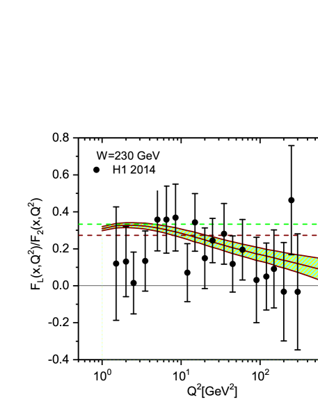
Figure 1: The ratio $F_{L}/F_{2}$ extracted at NNLO approximation in comparison with the H1 data [30] as accompanied with total errors. The results are presented at fixed value of the invariant mass W in the interval $1~{}\mathrm{GeV}^{2}\leq Q^{2}<3000~{}\mathrm{GeV}^{2}$ at low values of $x$. The shaded are correspondent to uncertainties of the $F_{2}$ parameterization (i.e., Table II). The dipole upper bounds represented by the dashed lines related to $\rho=1$ and $\frac{4}{3}$ respectively.

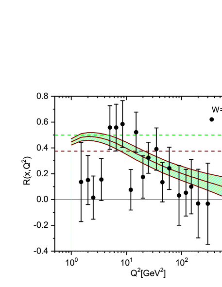
Figure 2: The same as Fig.1 for the ratio $R$.

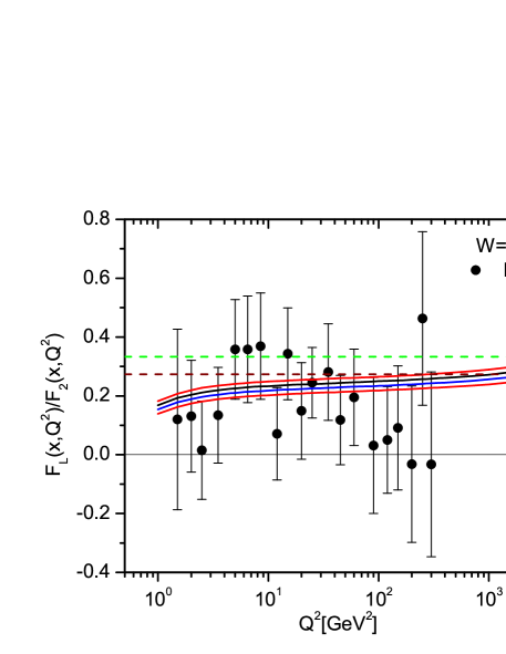
Figure 3: The ratio $F_{L}/F_{2}$ extracted at NNLO approximation in comparison with the H1 data [30] as accompanied with total errors. The results are presented at fixed value of the invariant mass W in the interval $1~{}\mathrm{GeV}^{2}\leq Q^{2}<3000~{}\mathrm{GeV}^{2}$ at low values of $x$. The solid lines are defined with the fixed exponents. The singlet exponents are a dynamical quantity of the order of $\lambda=0.27,29,31$ and $0.33$ from lower to upper curves respectively. The dipole upper bounds represented by the dashed lines related to $\rho=1$ and $\frac{4}{3}$ respectively.

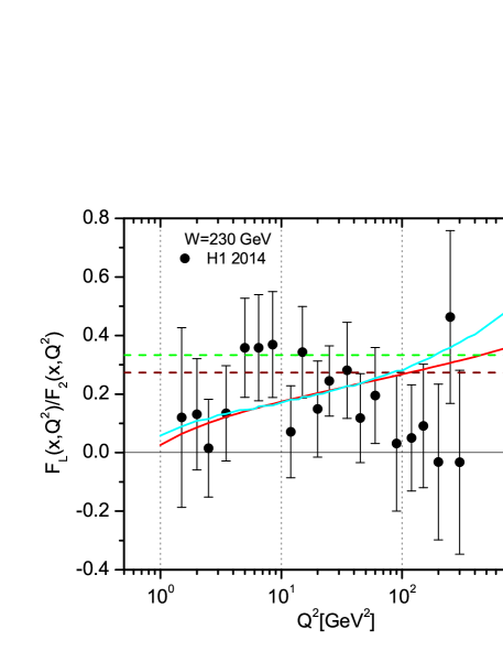
Figure 5: The ratio $F_{L}/F_{2}$ extracted at NNLO approximation in comparison with the H1 data [30] as accompanied with total errors. The results are presented at fixed value of the invariant mass W in the interval $1~{}\mathrm{GeV}^{2}\leq Q^{2}<3000~{}\mathrm{GeV}^{2}$ at low values of $x$. The solid lines are defined with respect to the effective singlet exponents. The exponents $\lambda^{s}(Q^{2})$ are parameterized as to Eqs.(40) and (41) from lower to upper curves respectively. The dipole upper bounds represented by the dashed lines related to $\rho=1$ and $\frac{4}{3}$ respectively.

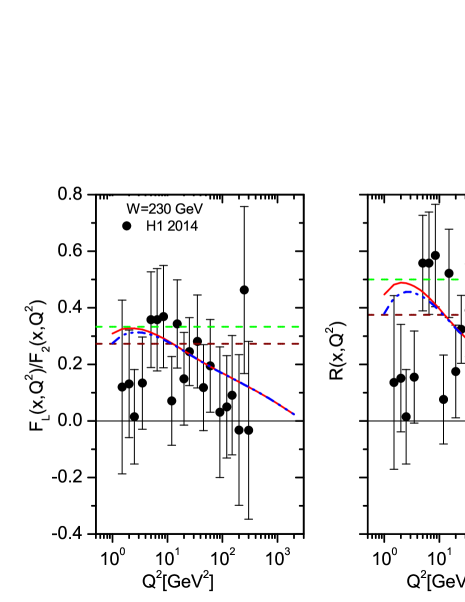
Figure 7: The nonlinear corrections to the ratio of structure functions (left, $F_{L}(x,Q^{2})/F_{2}(x,Q^{2})$) and (right, $R(x,Q^{2})$) extracted at NNLO approximation in comparison with the H1 data [16] as accompanied with total errors. The results are presented at fixed value of the invariant mass W in the interval $1~{}\mathrm{GeV}^{2}\leq Q^{2}<3000~{}\mathrm{GeV}^{2}$ at low values of $x$. The dash-dot line is defined with the nonlinear corrections in comparison with the linear (i.e., solid line). The dipole upper bounds represented by the dashed lines related to $\rho=1$ and $\frac{4}{3}$ respectively.

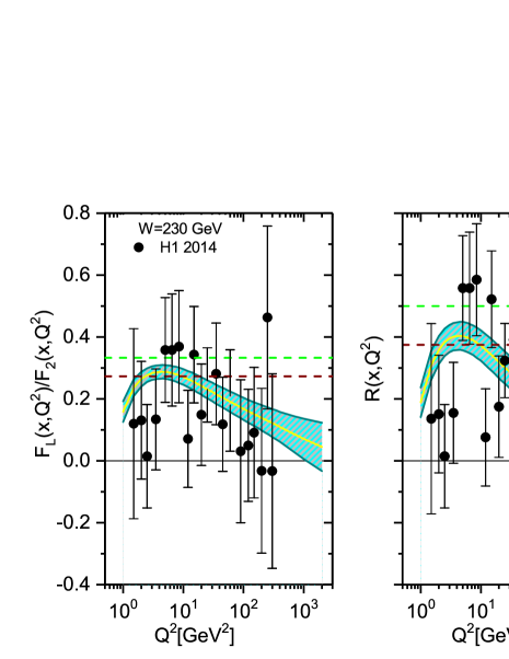
Figure 8: The nonlinear corrections to the ratio of structure functions (left, $F_{L}(x,Q^{2})/F_{2}(x,Q^{2})$) and (right, $R(x,Q^{2})$) with respect to the effective exponent $\lambda^{s}(Q^{2})$ [39] extracted at NNLO approximation in comparison with the H1 data [30] as accompanied with total errors. The results are presented at fixed value of the invariant mass W in the interval $1~{}\mathrm{GeV}^{2}\leq Q^{2}<3000~{}\mathrm{GeV}^{2}$ at low values of $x$. The error bands represent the uncertainty estimation coming from the $F_{2}$ parameterization. The dipole upper bounds represented by the dashed lines related to $\rho=1$ and $\frac{4}{3}$ respectively.

In this paper, we obtained the ratio of structure functions based on the $F_{2}$ parameterization and singlet exponent behavior at NNLO analysis. The behavior of ratios compared with HERA data and also with CDP bounds. We use the $F_{2}$ parameterized [33] where fitted to the combined H1 and ZEUS inclusive DIS data [35] in a range of the kinematical variables $x<0.01$ and $0.15~{}\mathrm{GeV^{2}}<Q^{2}<3000~{}\mathrm{GeV^{2}}$. The coupling constant defined via the $n_{f}=4$ definition of $\Lambda_{QCD}$ for the ZEUS data [35] and the MRST set of partons [42]. The values of $\Lambda_{QCD}$ at LO up to NNLO are displayed in Table III respectively. The values of $\lambda_{s}\simeq 0.33$ and $\lambda_{g}\simeq 0.43$ [43-46] are used within the range of $Q^{2}$ under study. The predictions for the ratio of structure functions have been depicted at fixed value of the invariant mass W (i.e. $W=230~{}\mathrm{GeV}$), and compared in the HERA kinematic range [5] at low values of $x$.
In Fig.1, we show the prediction of Eq.(31) for the ratio $F_{L}/F_{2}$ and compare this ratio with the H1 data [5] as accompanied with total errors. As can be seen in this figure, the depletion and enhancement in this ratio reflect the experimental data and it is comparable with the H1 data in the interval $1~{}\mathrm{GeV^{2}}<Q^{2}<500~{}\mathrm{GeV^{2}}$. The error bares are in accordance with the statistical errors of the $F_{2}$ parameterization as presented in Table II. Also a detailed comparison with the CDP bounds has been shown in this figure (i.e., Fig.1). As can be seen, the values of the ratio $F_{L}/F_{2}$ are in good agreement with the CDP bounds at $1<Q^{2}\leq 20~{}\mathrm{GeV}^{2}$ at fixed value of the invariant mass.
The ratio $R$ is expected to vanish at large $Q^{2}$ and moderate $x$ values in the naive parton model, but it is nonzero at low values of $x$. It dues to the fact that partons can carry transverse momentum [47]. In Fig.(2) we present the ratio $R$ related to Eq.(32) in comparison with the H1 data using the $F_{2}$ parameterization. As can be seen in this figure, one can conclude that the these results essentially improve the good agreement with data in comparison with the CDP bounds at the wide range of $Q^{2}$ values. We observe that this ratio is comparable with the CDP bounds at some values of $Q^{2}$ and it is compatible with the experimental data in a wide range of $Q^{2}$ values.
To emphasize the size of the CDP bounds we show that the ratio $F_{L}/F_{2}$ and $R$ have a maximum behavior when the proton structure function has a power law behavior. In Figs.(3) and (4) the ratio $F_{L}/F_{2}$ and $R$ obtained based on the gluon and singlet exponents at $W=230~{}\mathrm{GeV}$. These behaviors are in good agreements with the CDP bounds when applying the uncertainty principle at moderate $Q^{2}$ values. These results indicate a decrease of the ratios for small $Q^{2}$ values which it is require as to the electromagnetic gauge invariance. On the other hand, at large $Q^{2}$ values the exponent method is not consistent with the experimental data.
Therefore we study the ratio of structure functions with respect to the effective exponents. In Figs.(5) and (6) the ratio $F_{L}/F_{2}$ and $R$ are plotted as related to the singlet effective exponent $\lambda^{s}(Q^{2})$. It is seen that our results based on the effective exponent at NNLO approximation, over a wide range of $x$ and $Q^{2}$ values, are comparable with the experimental data at low and moderate $Q^{2}$ values. At high-$Q^{2}$ values, an overall shift between the HERA data and the predictions is observed. This behavior can be resolved with an adjustment of singlet exponent than one obtained with respect to the effective and phenomenological exponents via Eqs.(40) and (41) respectively.
The agreement between the method and the experimental data is good until $Q^{2}=200~{}\mathrm{GeV}^{2}$. Because the singlet effective exponents (i.e., Eqs.(40) and (41)) parameterized only for $Q^{2}<200~{}\mathrm{GeV}^{2}$. One can conclude that exponent defined for singlet distribution is larger than the gluon exponent at large $Q^{2}$ values where this behavior is not consistent with pQCD.
In figures (1) and (2) the behavior of the ratio $F_{L}/F_{2}$ and $R$ at low $Q^{2}$ should eventually be tamed by the nonlinear effects of the singlet density. The nonlinear corrections (NLCs) to the ratio ${F_{L}}/{F_{2}}$ and $R$ are considered in a wide range of $Q^{2}$ values in Fig.7. In this figure (i.e., Fig.7), the effects of nonlinearity are investigated in the hot-spot point ($R=2~{}\mathrm{GeV}^{-1}$) in comparison with the linear behavior from the $F_{2}$ parameterized. One can see that obtained nonlinear corrections for these ratios are observable at low $Q^{2}$ values ($1<Q^{2}<10~{}\mathrm{GeV}^{2}$) and comparable with the H1 data in a wide range of $Q^{2}$ values.
On the other hand, the nonlinear behaviors have been shown for the ratio ${F_{L}}/{F_{2}}$ and $R$ with respect to the singlet effective exponent $\lambda^{s}(Q^{2})$ in figure 8. The error bands represent the uncertainty estimation coming from the $F_{2}$ parameterized. As one can see in this plot, the inclusion of the nonlinear behavior by the effective exponent significantly change the behavior of the ratio of ${F_{L}}/{F_{2}}$ and $R$ in a wide range of $Q^{2}$ values. On can see an enhancement for the moderate value of $Q^{2}$ and reduction for the small and large values of $Q^{2}$. The results for the ratios clearly show significant agreement with the HERA data over a wide range of $x$ and $Q^{2}$ variables. The comparison of the results reveals the following conclusion: For a fixed value of the invariant mass $W$, one see the same patterns for the ratios when the effective exponent is $Q^{2}$-dependent. It is shown a pick around the moderate value of $Q^{2}$, $Q^{2}\sim 5~{}\mathrm{GeV}^{2}$. One of the main important results can be concluded from this figure is the significant reduction in the ratio ${F_{L}}/{F_{2}}$ and $R$ at low $Q^{2}$ values caused by including the nonlinear effects related to the singlet effective exponent in this analysis.

.6 6. Conclusion

We presented the high-order corrections for ratio $F_{L}/F_{2}$ and $R$ with respect to the derivative of the proton structure function into ${\ln}Q^{2}$. In this paper we have studied several aspect of the proton structure function behavior at small $x$. These ratios (i.e., $F_{L}/F_{2}$ and $R$) determined in the kinematical region where $F_{2}$ has been parameterized. The behavior of these ratios are in good agreement in comparison with the experimental data in a wide range of $Q^{2}$ values at a fixed invariant mass. The value of these ratios are different from the one obtained for the CDP bounds. Only at low $Q^{2}$ values these results are comparable with the CDP bounds. Then we have studied the effects of adding the nonlinear corrections to the ratio $F_{L}/F_{2}$ and $R$ in this region. These results are consistent with other experimental data, as we have discussed the meaning of this finding from the point of view of modified nonlinear behavior of these ratios.
Also a power-law behavior for the ratio of structure functions is predicted. The results for a fixed exponent are comparable with the CDP bounds and HERA data at moderate $Q^{2}$ values. At low and moderate $Q^{2}$ values an effective singlet exponent should be considered. This analysis is also enriched with considering the nonlinear contributions to the ratios related to the effective singlet exponent. We have therefore solved the ratio $F_{L}/F_{2}$ and $R$ with the nonlinear shadowing term included in order to determine the behavior of the effective singlet exponent at low values of $Q^{2}$. These results show that the data can be described in new colliders taking shadowing corrections to the effective exponent into account.

.7 ACKNOWLEDGMENTS

Authors are grateful the Razi University for financial support of this project and also G.R.Boroun is thankful the CERN theory department for their hospitality and support during the preparation of this paper.

.8 Appendix A

The kernels presented for the quark and gluon sectors, denoted by $\Phi$ and $\Theta$ respectively at LO up to NNLO,

$$\Theta_{qg}(x,Q^{2}) = P_{qg}(x,\alpha_{s})\otimes x^{\lambda_{g}},$$

$$\Phi_{qq}(x,Q^{2}) = P_{qq}(x,\alpha_{s})\otimes x^{\lambda_{s}},$$ (49)

have the following form at the leading order approximation as:

$$\Phi_{qq}(x,Q^{2}) = \frac{\alpha_{s}}{4\pi}\{4+\frac{16}{3}\ln(\frac{1-x}{x})+\frac{16}{3}\int_{x}^{1}{\frac{z^{\lambda_{s}}-{z}^{-1}}{1-z}dz}$$

$$-\frac{8}{3}\int_{x}^{1}{(1+z)z^{\lambda_{s}}dz\}},$$

$$\Theta_{qg}(x,Q^{2}) = \frac{\alpha_{s}}{4\pi}\frac{20}{9}\int_{x}^{1}{(z^{2}+(1-z)^{2})z^{\lambda_{g}}dz}.$$ (50)

Also the longitudinal kernels at low-$x$ limit presented by the following forms

$$I_{L,q}(x,Q^{2}) = \sum_{n=1}a(t)^{n}c_{L,q}^{n}(x)\otimes x^{\lambda_{s}},$$

$$I_{L,g}(x,Q^{2}) = \sum_{n=1}a(t)^{n}c_{L,g}^{n}(x)\otimes x^{\lambda_{g}}.$$ (51)

can be defined at leading order approximation by:

$$I_{L,q}(x,Q^{2}) = \frac{\alpha_{s}}{4\pi}\int_{x}^{1}8n_{f}(1-z)z^{\lambda_{s}+1}dz,$$

$$I_{L,g}(x,Q^{2}) = \frac{\alpha_{s}}{4\pi}\int_{x}^{1}4C_{F}z^{\lambda_{g}+1}dz.$$ (52)

Table 1: HERA data collected by two collaborations H1 and ZEUS.

HERA	$e^{+}p$	$e^{-}p$
HERA I	100 pb-1	15 pb-1
HERA II	150 pb-1	235 pb-1

Table 2: The effective Parameters at low $x$ for $0.15~{}\mathrm{GeV}^{2}<Q^{2}<3000~{}\mathrm{GeV}^{2}$ provided by the following values. The fixed parameters are defined by the Block-Halzen fit to the real photon-proton cross section as $M^{2}=0.753\pm 0.068~{}\mathrm{GeV}^{2}$ and $\mu^{2}=2.82\pm 0.290~{}\mathrm{GeV}^{2}$.

parameters                    value
$a_{00}$	$2.550\times 10^{-1}~{}\pm 1.60\times 10^{-2}$
$a_{01}$	$1.475\times 10^{-1}~{}\pm 3.025\times 10^{-2}$
$a_{10}$	$8.205\times 10^{-4}~{}~{}\pm 4.62\times 10^{-4}$
$a_{11}$	$-5.148\times 10^{-2}\pm 8.19\times 10^{-3}$
$a_{12}$	$-4.725\times 10^{-3}\pm 1.01\times 10^{-3}$
$a_{20}$	$2.217\times 10^{-3}\pm 1.42\times 10^{-4}$
$a_{21}$	$1.244\times 10^{-2}\pm 8.56\times 10^{-4}$
$a_{22}$	$5.958\times 10^{-4}\pm 2.32\times 10^{-4}$
$n$	$11.49\pm 0.99$
$\lambda$	$2.430~{}\pm 0.153$
$\chi^{2}(\mathrm{goodness~{}of~{}fit})$	$0.95$

Table 3: The QCD coupling and corresponding $\Lambda$ parameter for $n_{f}=4$ at LO, NLO [33, 43] and NNLO analysis [42].

	$\alpha_{s}(M_{Z}^{2})$	$\Lambda_{QCD}(MeV)$
LO	0.1166	136.8
NLO	0.1166	284
NNLO	0.1155	235

I References

1. M.Klein, arXiv [hep-ph]:1802.04317.
2. N.Armesto et al., Phys. Rev. D 100, 074022 (2019).
3. A. Abada et al., [FCC Collaborations], Eur.Phys.J.C79, 474(2019).
4. H.Abramowicz et al.,[H1 and ZEUS Collaborations], Eur.Phys.J.C75, 580(2015).
5. V.Andreev et al. [H1 Collaboration], Eur.Phys.J.C74, 2814 (2014).
6. A. H. Mueller and J. Qiu, Nucl. Phys. B268, 427(1986); L. V. Gribov, E. M. Levin and M. G. Ryskin, Phys. Rep.100, 1(1983).
7. G.R.Boroun and S.Zarrin, Eur.Phys.J.Plus 128, 119(2013); G. R. Boroun and B. Rezaei, Chin. Phys. Lett.32, 111101(2015); B. Rezaei and G. R. Boroun, Phys. Lett. B692, 247 (2010); G. R. Boroun, Eur. Phys. J. A43, 335(2010); G.R.Boroun, Eur.Phys.J. A42, 251 (2009).
8. M.Devee, arXiv[hep-ph]:1808.00899; M.Devee and J.K.sarma, Nucl.Phys. B885, 571(2014); M.Lalung et al., Nucl.Phys. A984, 29 (2019); P.Phukan et al., Nucl.Phys. A968, 275 (2017).
9. R.Wang and X.Chen, Chin.Phys. C41, 053103 (2017); J.Lan et al., arXiv[nucl-th]:1907.01509.
10. N. N. Nikolaev and W. Sch$\ddot{a}$fer, Phys. Rev. D74, 014023(2006).
11. M.Kuroda and D.Schildknecht, Phys.Lett. B618, 84(2005); M.Kuroda and D.Schildknecht, Acta Phys.Polon. B37, 835(2006).
12. M.Kuroda and D.Schildknecht, Phys.Lett. B670, 129(2008); M.Kuroda and D.Schildknecht, Phys.Rev. D96, 094013(2017).
13. D.Schildknecht and M.Tentyukov, arXiv[hep-ph]:0203028; M.Kuroda and D.Schildknecht, Phys.Rev. D85, 094001(2012).
14. D.Schildknecht, Mod.Phys.Lett.A29, 1430028(2014).
15. M.Kuroda and D.Schildknecht, Int. J. Mod. Phys. A31, 1650157 (2016).
16. Amir H.Rezaeian and I.Schmidt, Phys.Rev. D88, 074016 (2013).
17. J.R.Forshaw et al., JHEP 0611, 025(2006).
18. C.Ewerz et al., Phys.lett.B720, 181(2013).
19. C.Ewerz and O.Nachtmann, Phys.Lett.B648, 279(2007).
20. M.Niedziela and M.Praszalowicz, Acta Phys.Polon. B46, 2019(2015).
21. F.D. Aaron et al. [H1 Collaboration], phys.Lett.B665, 139(2008); Eur.Phys.J.C71,1579(2011).
22. C.Ewerz et al., Phys.Rev. D77, 074022(2008).
23. H.Abromowicz et al. [ZEUS Collaboration], Phys.Rev.D9, 072002(2014).
24. S.Moch, J.A.M.Vermaseren, A.Vogt, Phys.Lett.B 606, 123(2005).
25. W.L. van Neerven, A.Vogt, Phys.Lett.B 490, 111(2000).
26. A.Vogt, S.Moch, J.A.M.Vermaseren, Nucl.Phys.B 691, 129(2004).
27. Yu.L.Dokshitzer, Sov.Phys.JETP 46, 641(1977); G.Altarelli and G.Parisi, Nucl.Phys.B 126, 298(1977); V.N.Gribov and L.N.Lipatov, Sov.J.Nucl.Phys. 15, 438(1972).
28. V.S.Fadin, E.A.Kuraev and L.N.Lipatov, Phys.Lett.B 60, 50(1975); L.N.Lipatov, Sov.J.Nucl.Phys. 23, 338(1976); I.I.Balitsky and L.N.Lipatov, Sov.J.Nucl.Phys. 28, 822(1978).
29. G.R.Boroun and B.Rezaei, Nucl.Phys.A990, 244(2019).
30. B.Rezaei and G.R.Boroun, Eur.Phys.J.A55, 66(2019).
31. S.Moch, J.A.M.Vermaseren, A.Vogt, Phys.Lett.B 606, 123(2005).
32. G.R.Boroun, Phys.Rev. C97, 015206 (2018); G.R.Boroun and B.Rezaei, Eur.Phys.J. C72, 2221(2012).
33. M. M. Block, L. Durand and P. Ha, Phys. Rev.D89, no. 9, 094027 (2014).
34. L.P.Kaptari et al., Phys.Rev.D 99, 096019(2019).
35. F. D. Aaron et al. [H1 and ZEUS Collaborations], JHEP1001, 109(2010).
36. A. Donnachie, P.V. Landshoff, Phys. Lett. B 550, 160 (2002); B.Rezaei and G.R.Boroun , Int.J.Theor.Phys. 57, 2309(2018).
37. Martin M. Block et al., Phys. Rev. D 84 , 094010 (2011).
38. M. Praszalowicz, Phys. Rev. Lett. 106, 142002(2011).
39. M. Praszalowicz, T. Stebel, JHEP03, 090(2013).
40. H1 and ZEUS Collaboration (F.D. Aaron et al.), JHEP01, 109 (2010); H1 and ZEUS Collaboration (F.D. Aaron et al.), Eur. Phys. J. C 63, 625(2009); H1 and ZEUS Collaboration (F.D. Aaron et al.), Eur. Phys. J. C 64, 561(2009).
41. K. J. Eskola et al., Nucl. Phys. B660, 211(2003); R. Fiore, P. V. Sasorov and V. R. Zoller, JETP Letters 96, 687(2013); R. Fiore, N. N. Nikolaev and V. R. Zoller, JETP Letters 99, 363(2014).
42. A.D.Martin et al., Phys.Letts.B604, 61(2004).
43. S. Chekanov et al. [ZEUS Collaboration], Eur. Phys. J.C 21, 443 (2001).
44. K Golec-Biernat and A.M.Stasto, Phys.Rev.D 80, 014006(2009).
45. G.R.Boroun, Eur.Phys.J.Plus 135, 68(2020); G.R.Boroun and B.Rezaei, Eur.Phys.J. C73, 2412(2013); Phys.Atom.Nucl.71, 1077(2008); EPL100, 41001(2012).
46. A. Y. Illarionov, A. V. Kotikov and G. Parente Bermudez, Phys. Part. Nucl. 39, 307 (2008).
47. V.Tvaskis et al., Phys.Rev.C97, 045204(2018); Phys.Rev.Lett.98, 142301(2007).

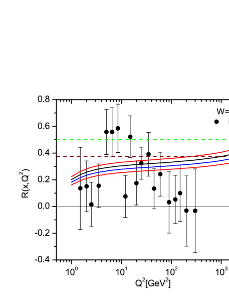
Figure 4: The same as Fig.3 for the ratio $R$.

Figure 6: The same as Fig.5 for the ratio $R$.