A finite-difference lattice Boltzmann model with second-order accuracy of time and space for incompressible flow

Abstract

In this paper, a kind of finite-difference lattice Boltzmann method with the second-order accuracy of time and space (T2S2-FDLBM) is proposed. In this method, a new simplified two-stage fourth order time-accurate discretization approach is applied to construct time marching scheme, and the spatial gradient operator is discretized by a mixed difference scheme to maintain a second-order accuracy both in time and space. It is shown that the previous finite-difference lattice Boltzmann method (FDLBM) proposed by Guo [1] is a special case of the T2S2-FDLBM. Through the von Neumann analysis, the stability of the method is analyzed and two specific T2S2-FDLBMs are discussed. The two T2S2-FDLBMs are applied to simulate some incompressible flows with the non-uniform grids. Compared with the previous FDLBM and SLBM, the T2S2-FDLBM is more accurate and more stable. The value of the Courant-Friedrichs-Lewy condition number in our method can be up to 0.9, which also significantly improves the computational efficiency.

1 Introduction

In the past 30 years, the lattice Boltzmann method (LBM) has received increasing attention, and also made great progress in the fields of microscale flows [2, 3, 4], porous media flows [5, 6], multiphase flows [7, 8, 9, 10, 11, 12] and turbulent flows [13, 14]. With the approach of the interpolation [15, 16], LBM can be implemented on nonuniform grids. In the LBM, the refinement scheme of non-uniform mesh mainly includes static mesh refinement [17, 18, 19] and dynamic mesh refinement [20, 21, 22, 23, 24]. In addition, there are several methods combined LBM with finite-difference [25, 26, 27, 24, 28], finite-volume [29, 30], finite-element approaches [31] and so on. These methods can promote the geometrical flexibility of the LBM. Unlike SLBM, the discrete-velocity in these methods is decoupled with lattice and time steps, and thus, the non-uniform meshes can be used to improve computational efficiency and accuracy of LBM.

In 1995, Reider and Sterling first proposed a finite-difference lattice Boltzmann equation (FDLBE) for the simulation of the incompressible Navier-Stokes equations [32], then Cao and Chen examined more details of FDLBE [33]. Mei and Shyy developed the FDLBM on curvilinear coordinates [34]. Based on this work, Guo et al. proposed an implicit treatment for collision term of the Bhatnagar-Gross-Krook Boltzmann equation, and presented a mixed difference scheme to discrete the advection term [1]. In addition, Guo et al. developed a new FDLBM for dense binary mixtures, where the second-order Lax Wendroff scheme and first-order Euler’s formula are used to discrete space and time derivatives, respectively [35]. Wang et al. proposed a high-order FDLBM to deal with the compressibility and non-linear shock wave effects in the resonator, in which a third-order implicit-explicit Runge-Kutta scheme and a fifth-order weighted essentially non-oscillatory (WENO) scheme are used for time and space discretization [36]. In 2013, Amin and Sun studied the stability condition of the FDLBM [37]. Subsequently, Kim and Yang incorporates the immersed boundary method into the FDLBM [38]. Besides, the multi-speed model was also combined with the FDLBM [39], and the work on FDLBM for three-dimensional incompressible flows [40] was also conducted.

Up to now, most of high-order FDLBMs are implemented by using Runge-Kutta scheme for time discretization, and fifth-order WENO scheme or fourth-order compact finite-difference scheme for space discretization [36, 41, 42, 43, 40]. The high-order FDLBMs can be used to improve the accuracy and convergent speed, but those methods are at the expense of overcomplicated calculation, which loses the simplicity of SLBM. Moreover, most of the current work on high order FDLBM are implemented on uniform grid which neglects the computational efficiency brought by non-uniform grids. In addition, the simple FDLBM proposed by Guo [1] retains the computational framework of SLBM, but the computational efficiency was not improved greatly. This limitation results from the value of Courant-Friedrichs-Lewy (CFL) condition number. In the implementation of FDLBM, CFL condition number is proportional to the time step. The theoretical range of CFL condition number is $(0,1)$, but it is usually around 0.1 in the numerical simulations. In contrast, the value of the CFL condition number is 1 in the SLBM. Compared with SLBM, the application of non-uniform grid in FDLBM may bring higher computational efficiency and accuracy, but the smaller value of CFL condition number will also influence the efficiency.

In order to solve this problem, a new FDLBM with a second-order accuracy both in space and time is proposed. To simplify following discussion, the FDLBM developed by Guo [1] is marked as T1S2-FDLBM, and the present FDLBM is denoted by T2S2-FDLBM. The theoretical analysis and numerical result show that T2S2-FDLBM has a second-order accuracy in space and time, and also, the value of the CFL condition number in T2S2-FDLBM can be increased up to 0.9. At the same time, with the application of non-uniform grid, the T2S2-FDLBM is more efficient and more accurate than SLBM and T1S2-FDLBM.

The rest of the paper is organized as follows. In Sec. 2, the T2S2-FDLBM is constructed from time and spatial discretization. We also analyze the stability of the method by Von Neumann analysis. Then some numerical simulation are conducted in Sec. 3, and finally, some conclusions are given in Sec. 4.

2 Numerical methods

In this section, the Boltzmann equation will be discreted by some different schemes. Inspired by Wu et al. [44], we use a new simplified two-stage fourth order time-accurate discretization (TFTD) method to construct the time marching scheme. And similar to the spatial discretization in [1], the gradient term is discreted by a mixed difference scheme which incorporates the central difference and the second-order upwind-difference schemes. Moreover, the Von Neumann analysis would be applied to evaluate the numerical stability of the T2S2-FDLBM and determine the model parameters.

A. Time discretization

The time-dependent Boltzmann equation with a force term can be written follows

$$\frac{{\partial f}}{\partial t}=L(f)+\bar{\Omega}(f):=M,$$ (1)

where f is particle distribution function. The gradient term L and $\bar{\Omega}$ can be expressed as

$$\ L(f)=-\bm{\xi}\cdot\nabla f,$$ (2)

$$\ \bar{\Omega}(f)=\Omega(f)+F,$$ (3)

where $\bm{\xi}$ represents the particle velocity and the $\bar{\Omega}$ contains the force term F and collision term $\Omega$. Integrating Eq. (1) over the time interval $[t_{n},t_{n}+\Delta t]$ yields

$$\ f^{n+1}=f^{n}+\int_{t_{n}}^{t_{n}+\Delta t}M[f(t)]dt,$$ (4)

where $f^{n}=f(\bm{x},\bm{\xi},t_{n})$. According to the previous work [45], the chain rule and Cauchy-Kovalevskaya theorem can be used to deal with time derivative of $M(f)$ at $t=t_{n}$,

$$\ \frac{\partial}{\partial t}M(f^{n})=M_{f}(f^{n})M(f^{n}),$$ (5)

where $M_{f}=dM/df$. To ensure the second-order accuracy in time, applying Taylor expansion to $M(f)$, we have

$$\begin{split}\ M(f)&=M(f^{n})+(t-t_{n})\frac{\partial}{\partial t}M(f^{n})+O(\triangle t^{2})\\ \ &=M(f^{n})+(t-t_{n})M_{f}(f^{n})M(f^{n})+O(\triangle t^{2}).\end{split}$$ (6)

Consequently, the time integral term in Eq. (4) can be approximated as

$$\ \int_{t_{n}}^{t_{n}+\Delta t}M(f)dt=\Delta tM(f^{n})+\frac{\Delta t^{2}}{2}M_{f}(f^{n})M(f^{n})+O(\Delta t^{3}).$$ (7)

Then, to construct a numerical scheme to Eq. (4), we introduce the intermediate variable $f^{*}=f(\bm{x},\bm{\xi},t_{*})$ at time $t_{*}=t_{n}+A\Delta t$. Using Taylor series analysis to the intermediate variable, we obtain

$$\ f^{*}=f^{n}+A\Delta tM(f^{n})+\frac{1}{2}A^{2}\Delta t^{2}\frac{\partial}{\partial t}M(f^{n})+O(\Delta t^{3}).$$ (8)

From Eq. (4), one can also have

$$\ f^{n+1} = f^{n}+\Delta t\left[B_{0}M(f^{n})+B_{1}M(f^{*})+B_{2}M(f^{n+1})\right],$$ (9)

$$\ f^{n+1} = f^{n}+\Delta t\left[B_{0}L(f^{n})+B_{1}L(f^{*})+B_{2}L(f^{n+1})\right]$$

$$+\Delta t\left[B_{0}\bar{\Omega}(f^{n})+B_{1}\bar{\Omega}(f^{*})+B_{2}\bar{\Omega}(f^{n+1})\right],$$ (10)

where $B_{0}$, $B_{1}$, $B_{2}$ and $A$ are adjustable parameters. By expanding the $f^{*}$ and $f^{n+1}$ at $f^{n}$, we have

$$\ \Delta t\left[B_{0}M(f^{n})+B_{1}M(f^{*})+B_{2}M(f^{n+1})\right]=\Delta t\left(B_{0}+B_{1}+B_{2}\right)M(f^{n})$$

$$+\frac{\Delta t^{2}}{2}\left[2(AB_{1}+B_{2})\right]M_{f}(f^{n})M(f^{n})+O(\Delta t^{3}).$$ (11)

Through a comparison of Eqs. (7) and (11), the following relations can be derived,

$$\ B_{0}+B_{1}+B_{2}=1,$$ (12a)

$$\ AB_{1}+B_{2}=\frac{1}{2},$$ (12b)

where $0\leq B_{0},B_{1},A\leq 1$ and $0\leq B_{2}\leq 1/2$. Here it should be noted that the number of equations is less than that of parameters, and two of those parameters can be adjusted flexibly. Besides, it is clear that Eq. (9) is a first-order scheme when only Eq. (12a) is satisfied, while it would be a second-order scheme when both Eqs. (12a) and (12b) are satisfied.

To generalize the method, the coefficients in $L(f)$ and $\bar{\Omega}(f)$ can be designed as follows,

$$\ f^{n+1} = f^{n}+\Delta t\left[\tilde{B_{0}}L(f^{n})+\tilde{B_{1}}L(f^{*})+\tilde{B_{2}}L(f^{n+1})\right]$$ (13)

$$+\Delta t\left[\bar{B_{0}}\bar{\Omega}(f^{n})+\bar{B_{1}}\bar{\Omega}(f^{*})+\bar{B_{2}}\bar{\Omega}(f^{n+1})\right].$$

Equation (10) can be considered as a special case of Eq. (13) when the parameters satisfy the relations, $\tilde{B_{0}}=\bar{B_{0}},\tilde{B_{1}}=\bar{B_{1}},\tilde{B_{2}}=\bar{B_{2}}.$ Similarly, after a comparison of Eqs. (8) and (13), we have

$$\tilde{B_{0}}+\tilde{B_{1}}+\tilde{B_{2}}=1,\bar{B_{0}}+\bar{B_{1}}+\bar{B_{2}}=1,$$ (14a)

$$A\tilde{B_{1}}+\tilde{B_{2}}=\frac{1}{2},A\bar{B_{1}}+\bar{B_{2}}=\frac{1}{2},$$ (14b)

where $0\leq\tilde{B_{0}},\tilde{B_{1}},A\leq 1$, $0\leq\tilde{B_{2}}\leq 1/2$ and $0\leq\bar{B_{0}},\bar{B_{1}},A\leq 1$, $0\leq\bar{B_{2}}\leq 1/2$.

Remark I. We noted that T1S2-FDLBM is a special case of Eq. (13). Actually, according to Eq. (14a), the T1S2-FDLBM in Ref [1] can be obtained when the following relations are satisfied,

$$A=0,\tilde{B_{0}}=1,\tilde{B_{1}}=\tilde{B_{2}}=0,\bar{B_{0}}=\frac{1}{2},\bar{B_{1}}=0,\bar{B_{2}}=\frac{1}{2}.$$ (15)

The evolution equation of T1S2-FDLBM reads

$$f^{n+1}=f^{n}+\Delta tL(f^{n})+\frac{1}{2}\Delta t\left[\bar{\Omega}(f^{n})+\bar{\Omega}(f^{n+1})\right]+O(\Delta t^{2}).$$ (16)

We would like to point out that Eq. (16) can be rewritten in an explicit form,

$$\tilde{f}^{n+1}=\tilde{f}^{+,n}+\Delta tL(f^{n})+O(\Delta t^{2}),$$ (17)

where

$$\tilde{f}=f-\frac{1}{2}\Delta t\bar{\Omega},$$ (18)

$$\tilde{f}^{+}=f+\frac{1}{2}\Delta t\bar{\Omega}=\frac{2\tau-\Delta t}{2\tau+\Delta t}\tilde{f}+\frac{2\Delta t}{2\tau+\Delta t}f^{eq}+\frac{2\tau\Delta t}{2\tau+\Delta t}F.$$ (19)

In order to construct a second-order time marching scheme of FDLBM, there are two sets of parameters need to be considered (we refer the reader to section C for details). The first one is designed as

$$A=\frac{1}{2},\tilde{B_{0}}=0,\tilde{B_{1}}=1,\tilde{B_{2}}=0,\bar{B_{0}}=\frac{1}{2},\bar{B_{1}}=0,\bar{B_{2}}=\frac{1}{2},$$ (20)

and the corresponding evolution equation can be rewritten as

$$f^{n+1}=f^{n}+\Delta tL(f^{*})+\frac{1}{2}\Delta t\left[\bar{\Omega}(f^{n})+\bar{\Omega}(f^{n+1})\right]+O(\Delta t^{2}).$$ (21)

In addition, we can also determine the other one as

$$\tilde{B_{0}}=\frac{1}{2},\tilde{B_{1}}=0,\tilde{B_{2}}=\frac{1}{2},\bar{B_{0}}=\frac{1}{2},\bar{B_{1}}=0,\bar{B_{2}}=\frac{1}{2},\quad for\quad A\in[0,1],$$ (22)

and the evolution equation can also be obtain,

$$f^{n+1}=f^{n}+\frac{\Delta t}{2}(L(f^{n})+L(f^{n+1}))+\frac{1}{2}\Delta t\left[\bar{\Omega}(f^{n})+\bar{\Omega}(f^{n+1})\right]+O(\Delta t^{2}).$$ (23)

Similarly to Eq. (16), Eqs. (21) and (23) can also be written in the explicit forms,

$$\tilde{f}^{n+1}=\tilde{f}^{+,n}+\Delta tL(f^{*})+O(\Delta t^{2}),$$ (24)

$$\tilde{f}^{n+1}=\tilde{f}^{+,n}+\frac{\Delta t}{2}(L(f^{n})+L(f^{n+1}))+O(\Delta t^{2}).$$ (25)

To make a distinction between two T2S2-FDLBMs, the first one described by Eq. (24) is denoted by T2S2-FDLBM1, while the second one given by Eq. (25) is marked as T2S2-FDLBM2.

B. Space discretization

Here the method of integrating along the characteristic line is used to calculate the distribution function at intermediate moment. The discrete form of Eq. (1) can be expressed as

$$\tilde{f}^{n+1}_{i}=\tilde{f}^{+,n}_{i}+\Delta tL(f_{i}^{*}),$$ (26)

or

$$\tilde{f}^{n+1}_{i}=\tilde{f}^{+,n}_{i}+\frac{\Delta t}{2}(L(f_{i}^{n})+L(f_{i}^{n+1})),$$ (27)

where $f_{i}^{n}=f(\bm{x},\xi_{i},t_{n})$, and the gradient terms can be rewritten as

$$L(f_{i})=-\bm{\xi}_{i}\cdot\nabla f_{i}=-\xi_{i\alpha}\frac{\partial f_{i}}{\partial\chi_{\alpha}},$$ (28)

where $f_{i}$ represents the distribution function $f^{n}_{i}$, $f^{n+1}_{i}$ or $f^{*}_{i}$. Therefore, the evaluation of the distribution function $f^{*}_{i}$ or $f^{n+1}_{i}$ is the key to calculate the gradient term. Considering the following Boltzmann equation,

$$\frac{\partial f_{i}}{\partial t}+\bm{\xi}_{i}\cdot\nabla f_{i}=\bar{\Omega_{i}},$$ (29)

and integrating Eq. (29) along the characteristic line $x+\xi_{i}t$ over $[0,h]$, we have

$$f(\bm{x}+\bm{\xi}_{i}t,\xi_{i},t)-f(\bm{x},\bm{\xi}_{i},t)=\int^{h}_{0}\bar{\Omega}(\bm{x}+\bm{\xi}_{i}s,\bm{\xi}_{i},s)ds,$$ (30)

where $h$ is the time step, $h=\Delta t/2$ in the T2S2-FDLBM1, and $h=\Delta t$ in the T2S2-FDLBM2.

When the trapezoidal formula is applied to approximate the integral of the collision term in Eq. (30), we can obtain

$$f(\bm{x},\bm{\xi}_{i},t+h)-f(\bm{x}-\bm{\xi}_{i}h,\bm{\xi}_{i},t)=\frac{h}{2}\left[\bar{\Omega}(\bm{x},\bm{\xi}_{i},t+h)+\bar{\Omega}(\bm{x}-\bm{\xi}_{i}h,\bm{\xi}_{i},t)\right].$$ (31)

Introducing a new variable $\bar{f}_{i}$,

$$\bar{f}_{i}=f_{i}-\frac{h}{2}\bar{\Omega}_{i},$$ (32)

or equivalently,

$$f_{i}=\frac{2\tau}{2\tau+h}\bar{f}_{i}+\frac{h}{2\tau+h}f_{i}^{eq}+\frac{h\tau}{2\tau+h}F_{i},$$ (33)

we can rewrite Eq. (31) as

$$\bar{f}(\bm{x},\bm{\xi}_{i},t+h)=\bar{f}^{+,h}(\bm{x}-\bm{\xi}_{i}h,\bm{\xi}_{i},t),$$ (34)

where

$$\bar{f}_{i}^{+,h}=f_{i}+\frac{h}{2}\bar{\Omega}_{i}=\frac{2\tau-h}{2\tau+h}\bar{f}_{i}+\frac{2h}{2\tau+h}f_{i}^{eq}+\frac{2h\tau}{2\tau+h}F_{i}.$$ (35)

To ensure that the Eq. (26) achieves a second-order accuracy, the term $L(f_{i}^{*})$ should have a first-order accuracy. With the Taylor expansion, we can express $\bar{f}^{+,h}(\bm{x}-\bm{\xi}_{i}h,\bm{\xi}_{i},t)$ as

$$\bar{f}^{+,h}(\bm{x}-\bm{\xi}_{i}h,\bm{\xi}_{i},t)=\bar{f}^{+,h}(\bm{x},\bm{\xi}_{i},t)-h\xi_{i}\nabla\cdot\bar{f}^{+,h}(\bm{x},\bm{\xi}_{i},t).$$ (36)

In order to simplify the calculation, we use the same difference scheme to deal with the gradient terms in Eqs. (26), (27) and (36). Usually, the gradient term can be approximated by the central difference or upwind-difference schemes. However, the second-order upwind-difference scheme is more stable and the central-difference scheme has smaller numerical dispersion for high Reynolds number problems. For this reason, a mixed-difference scheme which combines the central-difference and second-order upwind difference schemes is adopted here,

$$\frac{\partial f_{i}}{\partial\chi_{\alpha}}\Bigg{|}_{m}=\eta\frac{\partial f_{i}}{\partial\chi_{\alpha}}\Bigg{|}_{c}+(1-\eta)\frac{\partial f_{i}}{\partial\chi_{\alpha}}\Bigg{|}_{u},$$ (37)

where $f_{i}$ represents $f_{i}^{*}$ or $\bar{f}_{i}^{+,h}$, and the parameter $\eta\in[0,1]$. The terms $\dfrac{\partial f_{i}}{\partial\chi_{\alpha}}\Bigg{|}_{u}$ and $\dfrac{\partial f_{i}}{\partial\chi_{\alpha}}\Bigg{|}_{c}$ represent second up-wind difference and central-difference schemes, and they are defined as

$$\frac{\partial f_{i}}{\partial\chi_{\alpha}}\Bigg{|}_{c}=\frac{f_{i}(\chi_{\alpha}+\Delta\chi_{\alpha},t)-f_{i}(\chi_{\alpha}-\Delta\chi_{\alpha},t)}{2\Delta\chi_{\alpha}},$$ (38)

$$\frac{\partial f_{i}}{\partial\chi_{\alpha}}\Bigg{|}_{c}=\begin{cases}\dfrac{3f_{i}(\chi_{\alpha},t)-4f_{i}(\chi_{\alpha}-\Delta\chi_{\alpha},t)+f_{i}(\chi_{\alpha}-2\Delta\chi_{\alpha},t)}{2\Delta\chi_{\alpha}},\quad&if\quad{c_{i\alpha}\geq 0},\\ -\dfrac{3f_{i}(\chi_{\alpha},t)-4f_{i}(\chi_{\alpha}+\Delta\chi_{\alpha},t)+f_{i}(\chi_{\alpha}+\Delta\chi_{\alpha},t)}{2\Delta\chi_{\alpha}},\quad&if\quad{c_{i\alpha}<0}.\end{cases}$$ (39)

C. Analysis of the T2S2-FDLBM

In this part, the von Neumann method is used to analyzed the numerical stability of the T2S2-FDLBM, and the force term is ignored to simplify the analysis. The evolution equation (13) can be rewritten as

$$\begin{split}\ f^{n+1}_{i}&=f^{n}_{i}+\Delta t\left[\tilde{B_{0}}L(f^{n}_{i})+\tilde{B_{1}}L(f^{*}_{i})+\tilde{B_{2}}L(f^{n+1}_{i})\right]\\ &+\Delta t\left[\bar{B_{0}}\Omega(f^{n}_{i})+\bar{B_{1}}\Omega(f^{*}_{i})+\bar{B_{2}}\Omega(f^{n+1}_{i})\right].\end{split}$$ (40)

According to the fact $f(\bm{x},\bm{\xi}_{i},t+h)=f(\bm{x},\bm{\xi}_{i},t)+h\partial_{t}f^{eq}(\bm{x},\bm{\xi}_{i},t)+O(h^{2})$ [46], expanding $f_{i}^{*}$ in Eq. (40) yields

$$\begin{split}\ &f^{n+1}_{i}-\Delta t\bar{B_{2}}\Omega(f^{n+1}_{i})-\Delta t\tilde{B_{2}}L(f^{n+1}_{i})=f^{n}_{i}+\Delta t(1-\bar{B_{2}})\Omega(f^{n}_{i})\\ &+\Delta t(1-\tilde{B_{2}})L(f^{n}_{i})+\Delta t(\frac{1}{2}-\tilde{B_{2}})L(\Delta t\partial_{t}f_{i}^{eq,n})-\omega(\frac{1}{2}-\bar{B_{2}})\Delta t\partial_{t}f_{i}^{eq,n}.\end{split}$$ (41)

where $f_{i}^{eq,n}=f^{eq}(\bm{x},\bm{\xi}_{i},t_{n})$. Then if the Euler formula is used to deal with time derivative, one can obtain

$$\begin{split}\ &f^{n+1}_{i}-\Delta t\bar{B_{2}}\Omega(f^{n+1}_{i})+\omega(\frac{1}{2}-\bar{B_{2}})f_{i}^{eq,n+1}+\Delta t\tilde{B_{2}}\xi\cdot\nabla f^{n+1}_{i}=\\ &-\Delta t(\frac{1}{2}-\tilde{B_{2}})\xi\cdot\nabla f^{eq,n+1}_{i}+f^{n}_{i}+\Delta t(1-\bar{B_{2}})\Omega(f^{n}_{i})-\Delta t(1-\tilde{B_{2}})\xi\cdot\nabla f^{n}_{i}\\ &+\Delta t(\frac{1}{2}-\tilde{B_{2}})\xi\cdot\nabla f^{eq,n}_{i}+\omega(\frac{1}{2}-\bar{B_{2}})f_{i}^{eq,n},\end{split}$$ (42)

where $\omega=\Delta t/\tau$. To conduct a linear stability analysis, $f_{i}$ is expanded as

$$f_{i}(\bm{x},t)=\overline{f_{i}^{eq}(\bm{x},t)}+f^{\prime}_{i}(\bm{x},t),$$ (43)

where $\overline{f_{i}^{eq}(\bm{x},t)}$ represents the global equilibrium distribution. It only depends on the mean value of density $\rho$ and velocity $u$, and does not vary with time and space. $f^{\prime}_{i}$ is the fluctuating quantity of $f_{i}$. With the help of Eq. (43), Eq. (42) can be written as

$$\begin{split}[(1+\omega\bar{B_{2}})\delta_{ij}+\omega(\frac{1}{2}-2\bar{B_{2}})\Gamma_{ij}]f^{\prime n+1}_{j}+[\tilde{B_{2}}\delta_{ij}+(\frac{1}{2}-\tilde{B_{2}})\Gamma_{ij}]\Delta t\bm{\xi}\cdot\nabla f^{\prime n+1}_{i}=&\\ +{[1-\omega(1-\bar{B_{2}})]\delta_{ij}+\omega(\frac{3}{2}-2\bar{B_{2}})\Gamma_{ij}}f^{\prime n}_{j}&\\ -[(1-\tilde{B_{2}})\delta_{ij}-(\frac{1}{2}-\tilde{B_{2}})\Gamma_{ij}]\Delta t\bm{\xi}\cdot\nabla f^{\prime n}_{i},&\end{split}$$ (44)

where $f_{j}^{\prime n}=f^{\prime}(\bm{x},\bm{\xi}_{j},t_{n})$ and $\Gamma_{ij}=\partial f_{i}^{eq}(\bm{x},t)/\partial f_{j}(\bm{x},t)$. With the Fourier transform, one can also get

$$F_{j}(\bm{k},t+\Delta t)=G_{ij}F_{j}(\bm{k},t),$$ (45)

where $F_{j}(\bm{k},t)=\int f^{\prime}_{j}(\bm{x},t)\exp(-i\bm{k}\cdot\bm{x})d\bm{x}$ and the wave number $\bm{k}=(k_{x},k_{y})$. The growth matrix $\bm{G}$ can be expressed as

$$\begin{split}\bm{G}&=\left\{(1+\omega\bar{B_{2}})\bm{I}+\omega(\frac{1}{2}-2\bar{B_{2}})\bm{\Gamma}+[\tilde{B_{2}}\bm{I}+(\frac{1}{2}-\tilde{B_{2}})\bm{\Gamma}]r\bm{S}\right\}^{-1}\\ &\times\left\{[1-\omega(1-\bar{B_{2}})]\bm{I}+\omega(\frac{3}{2}-2\bar{B_{2}})\bm{\Gamma}-[(1-\tilde{B_{2}})\bm{I}-(\frac{1}{2}-\tilde{B_{2}})\bm{\Gamma}]r\bm{S}\right\},\end{split}$$ (46)

where $r=\Delta t/\Delta x$ and $\bm{S}=diag(s_{0},s_{1},...s_{q})$ depends on $L(f)$. In the mixed difference scheme,

$$\begin{split}s_{j}=&l(1-\eta)(\sin\vartheta_{jx}+\sin\vartheta_{jy})+\frac{\eta}{2}[6-4\exp(-\vartheta_{jx})-4\exp(-\vartheta_{jy})\\ &+\exp(-2l\vartheta_{jx})+\exp(-2l\vartheta_{jy})],\end{split}$$ (47)

where $l^{2}=-1$, $\vartheta_{jx}=\kappa_{x}\xi_{jx}\Delta\chi$ and $\vartheta_{jy}=\kappa_{y}\xi_{jy}\Delta\chi$.

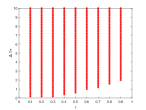
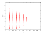
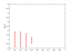
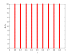
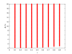
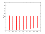
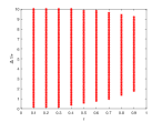
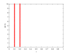
Figure 1: Stability regions of T2S2-FDLBM at different values of $\bar{B_{2}}$, $\tilde{B_{2}}$ and $\eta$. *, stable point: (a)$\tilde{B_{2}}=0$ $\eta=0.1$ and $\bar{B_{2}}=0.5,0.25,0$ (from left to right). (b) $\bar{B_{2}}=0.5$, $\eta=0.1$ and $\tilde{B_{2}}=0.5,0.25,0$ (from left to right). (c) $\bar{B_{2}}=0.5$, $\tilde{B_{2}}=0$ and $\eta=0,0.1,1$ (from left to right).

According to the stability condition, the spectral radius of the growth matrix $\bm{G}$ is required to be less than 1. From Eq. (46), it is clear that the spectral radius of the matrix $\bm{G}$ depends on the parameter of collision term ($\bar{B_{2}}$), the parameter of spatial gradient term ($\tilde{B_{2}}$), the weight coefficient of mixed scheme ($\eta$), and other four parameters $\bm{k}$, $\omega$, $r$ and $\bm{u}$. To perform an analysis of the numerical stability, the parameters $\bar{B_{2}}$, $\tilde{B_{2}}$ and $\eta$ are specified and $\bm{u}=(0.2,0.2)$, $0\leq\kappa_{\alpha}\Delta\chi\leq\pi$ $(\alpha=x,y)$. As shown in Fig. 1, the stability region is related to $r$ and $\omega$, and it is obvious that the present method can obtain a largest stability region when $\bar{B_{2}}=0.5$, $\tilde{B_{2}}=0.5$ and $\eta=0.1$. Moreover, taking account of computational efficiency, the method with $\bar{B_{2}}=0.5$, $\tilde{B_{2}}=0$ and $\eta=0.1$ is also worthing conducting a further study.

D. Computational sequence of two T2S2-FDLBMs

Fig. 2 is a flow chart of T2S2-FDLBM1, in which several steps are included.

Step (1). Estimate $L(f_{i}^{*})$ from $\tilde{f}_{i}^{n}$ through the method of integrating along the characteristic line,

$$\tilde{f}(\bm{x},\bm{\xi}_{i},t_{n})\stackrel{{\scriptstyle\eqref{eq:2.51}}}{{\longrightarrow}}\bar{f}^{+,h}(\bm{x},\bm{\xi}_{i},t_{n})\stackrel{{\scriptstyle\eqref{eq:2.33},\eqref{eq:2.35}}}{{\longrightarrow}}\bar{f}(\bm{x},\bm{\xi}_{i},t^{*})\stackrel{{\scriptstyle\eqref{eq:2.52}}}{{\longrightarrow}}f(\bm{x},\bm{\xi}_{i},t^{*})\stackrel{{\scriptstyle\eqref{eq:2.27},\eqref{eq:2.36}}}{{\longrightarrow}}L(f_{i}^{*}),$$

$$\bar{f}_{i}^{+,h}=\frac{4\tau-\Delta t}{4\tau+2\Delta t}\tilde{f}_{i}+\frac{3\Delta t}{4\tau+2\Delta t}f_{i}^{eq},$$ (48)

$$f_{i}=\frac{2\tau}{2\tau+h}\bar{f}_{i}+\frac{h}{2\tau+h}f_{i}^{eq}.$$ (49)

Step (2). Calculate $\tilde{f}_{i}^{+,n}$ from $\tilde{f}_{i}^{n}$ by Eq. (19),

$$\tilde{f}(\bm{x},\bm{\xi}_{i},t_{n})\stackrel{{\scriptstyle\eqref{eq:2.20}}}{{\longrightarrow}}\tilde{f}^{+}(\bm{x},\bm{\xi}_{i},t_{n}).$$

Step (3). Calculate $\tilde{f}^{n+1}$ from $L(f^{*})$ and $\tilde{f}^{+,n}$ by Eq. (24),

$$L(f_{i}^{*}),\tilde{f}^{+}(\bm{x},\bm{\xi}_{i},t_{n})\stackrel{{\scriptstyle\eqref{eq:2.23}}}{{\longrightarrow}}\tilde{f}(\bm{x},\bm{\xi}_{i},t_{n+1}).$$

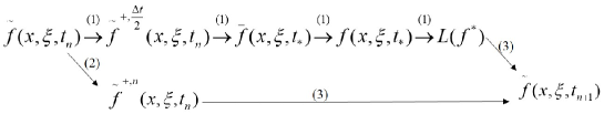
Figure 2: Flow chart of T2S2-FDLBM1.

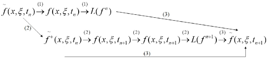
Figure 3: Flow chart of T2S2-FDLBM2.

Similarly, we also presented computational process of T2S2-FDLBM2 in Fig. 3, where the details are displayed as follows.

Step (1). Estimate $L(f_{i}^{n})$ from $\tilde{f}_{i}^{n}$,

$$\tilde{f}(\bm{x},\bm{\xi}_{i},t_{n})\stackrel{{\scriptstyle\eqref{eq:2.52}}}{{\longrightarrow}}f(\bm{x},\bm{\xi}_{i},t_{n})\stackrel{{\scriptstyle\eqref{eq:2.27},\eqref{eq:2.36}}}{{\longrightarrow}}L(f_{i}^{n}).$$

Step (2). Calculate $L(f_{i}^{n+1})$ from $\tilde{f}_{i}^{n}$,

$$\begin{split}&\tilde{f}\bm{x},\bm{\xi}_{i},t_{n})\stackrel{{\scriptstyle\eqref{eq:2.20}}}{{\longrightarrow}}\tilde{f}^{+}(\bm{x},\bm{\xi}_{i},t_{n})\stackrel{{\scriptstyle\eqref{eq:2.33},\eqref{eq:2.35}}}{{\longrightarrow}}\bar{f}(\bm{x},\bm{\xi}_{i},t^{n+1})\\ &\stackrel{{\scriptstyle\eqref{eq:2.52}}}{{\longrightarrow}}f(\bm{x},\bm{\xi}_{i},t_{n+1})\stackrel{{\scriptstyle\eqref{eq:2.27},\eqref{eq:2.36}}}{{\longrightarrow}}L(f_{i}^{n+1}).\end{split}$$

Step (3). Calculate $\tilde{f}_{i}^{n+1}$ from $L(f_{i}^{n})$, $L(f_{i}^{n+1})$ and $\tilde{f}_{i}^{+,n}$ by Eq. (25),

$$L(f_{i}^{n}),L(f_{i}^{n+1}),\tilde{f}^{+}(\bm{x},\bm{\xi}_{i},t_{n})\stackrel{{\scriptstyle\eqref{eq:5.23}}}{{\longrightarrow}}\tilde{f}(\bm{x},\bm{\xi}_{i},t_{n+1}).$$

In the implementation, $\bar{f}_{i}=\tilde{f}_{i}$ and $\bar{f}_{i}^{+,h}=\tilde{f}_{i}^{+}$ when $h=\Delta t$. Here it should be noted that the computational cost of T2S2-FDLBM2 is larger than T2S2-FDLBM1. The main reason is that two terms $L(f_{i}^{n})$ and $L(f_{i}^{n+1})$ should be calculated in T2S2-FDLBM2, while only $L(f_{i}^{n})$ needs to be calculated in T2S2-FDLBM1.

3 Numerical simulation

In this section, the Taylor vortex flow, the Poiseuille flow and the lid-driven flow will be used to test the two T2S2-FDLBMs.

Unless otherwise stated, in our simulations the equilibrium distribution function is adopted to initialize the distribution function, and the time step $\triangle t$ is given by the $CFL$ condition number,

$$\triangle t=CFL\frac{\triangle x}{\xi},$$ (50)

where $\triangle x$ is the minimum grid scale, and $\xi=\max|\bm{\xi}_{i}|$. $CFL$ condition number is an important parameter to evaluate the stability and convergence of method. The collision term $\Omega$ can be approximated by the simple single-relaxation-time Bhatnagar-Gross-Krook model,

$$\ \Omega(f_{i})=-\frac{{1}}{\tau}[f_{i}-f_{i}^{eq}],$$ (51)

where the equilibrium distribution function $f_{i}^{eq}$ in SLBM is defined as

$$\ f_{i}^{eq}=\omega_{i}\rho\left[1+\frac{{\bm{\xi}_{i}\cdot\bm{u}}}{c_{s}^{2}}+\frac{{\bm{uu}:(\bm{\xi}_{i}\bm{\xi}_{i}-c_{s}^{2}\textbf{I})}}{2c_{s}^{4}}\right],$$ (52)

and $f_{i}^{eq}$ in He-Luo model [47]can be also combined with this two T2S2-FDLBMs. The discrete particle velocities and corresponding weights are dependent on the lattice structure. For example,
D1Q3:

$$\begin{split}&\bm{\xi}_{i}=(0,1,-1)\xi,\\ &\omega_{0}=\frac{2}{3},\omega_{1}=\omega_{2}=\frac{1}{6},c_{s}^{2}=\frac{\xi^{2}}{3},\end{split}$$ (53)

D2Q9:

$$\begin{split}&\bm{\xi}_{i}=\left(\begin{array}[]{ccccccccc}0&1&0&-1&0&1&-1&-1&1\\ 0&0&1&0&-1&1&1&-1&-1\\ \end{array}\right)\xi,\\ &\omega_{i}=\left(\begin{array}[]{ccccccccc}\dfrac{4}{9}&\dfrac{1}{9}&\dfrac{1}{9}&\dfrac{1}{9}&\dfrac{1}{9}&\dfrac{1}{36}&\dfrac{1}{36}&\dfrac{1}{36}&\dfrac{1}{36}\\ \end{array}\right),c_{s}^{2}=\frac{\xi^{2}}{3}.\end{split}$$ (54)

The macroscopic density $\rho$ and velocity u can be obtained from the distribution function,

$$\ \rho=\Sigma\tilde{f_{i}},\quad\rho\textbf{u}=\Sigma\bm{\xi}_{i}\tilde{f_{i}}+\frac{1}{2}\Delta t\rho\bar{F},$$ (55)

where $\bar{F}$ represents the external force. According to the previous work [48], the force term in T2S2-FDLBM can be expressed as

$$\ F_{i}=\bar{F}\cdot(\xi_{i}-u)f_{i}^{eq}/(RT).$$ (56)

A. The Taylor vortex flow

The two-dimensional Taylor vortex flow is a periodic problem, and it is widely used to test the accuracy of the model. The analytical solution of the Taylor vortex flow is given by

$$\begin{split}u&=-u_{0}\cos(k_{1}x)\sin(k_{2}y)\exp\left[-\nu(k_{1}^{2}+k_{2}^{2})t\right],\\ v&=u_{0}\frac{k_{1}}{k_{2}}\sin(k_{1}x)\cos(k_{2}y)\exp\left[-\nu(k_{1}^{2}+k_{2}^{2})t\right],\\ p&=p_{0}-\frac{u_{0}^{2}}{4}\left[\cos(2k_{1}x)+\frac{k_{1}^{2}}{k_{2}^{2}}\cos(2k_{2}y)\right]\exp\left[-\nu(k_{1}^{2}+k_{2}^{2})t\right],\end{split}$$ (57)

where $u$ and $v$ are horizontal and vertical velocities of the fluid, $p$ is the pressure. The computational domain of the problem is set as $-\pi\leq x,y\leq\pi$, the mesh size is chosen to be $Nx\times Ny=32\times 128$, $k_{1}=1.0$, $k_{2}=4.0$, $u_{0}$ is set to be $0.01$. The time step is chosen to be $\pi/640$, and the shear viscosity $\nu$ is set as 0.001. The density can be initialized by $\rho=\rho_{0}+\delta p/c_{s}^{2}$, the average density $\rho_{0}=p_{0}/c_{s}^{2}$ and $\delta p=p-p_{0}$. For this time-dependence problem, the initial distribution function is given by [1],

$$\tilde{f}_{i}(\bm{x},\bm{\xi},t_{0})=f_{i}^{eq}(\bm{x},\bm{\xi},t_{0})-\frac{\rho_{0}\omega_{i}\tau(2+\Delta t)}{2c_{s}^{2}}\bm{\xi}_{i}\bm{\xi}_{i}:\nabla\bm{u}(\bm{x},\xi,t_{0}),$$ (58)

where $\rho_{0}$ and $u$ are determined by analytical solution.

Two T2S2-FDLBMs are first used to simulate the Taylor vortex flow, and the gradient term is discretized by three difference schemes: second-order upwind, central and mixed difference schemes ($\eta=0.01$). The results of three difference schemes are shown in Fig. 4. It can be observed from Fig. 4 that the T2S2-FDLBM1 with the up-wind difference scheme has a significant error, while the T2S2-FDLBM1 with the central difference or mixed difference scheme agree well with the analytical solution. Besides, from Fig. 4, one can also find that the results of T2S2-FDLBM1 and T2S2-FDLBM2 are in good agreement with the analytical solution when $CFL=0.1$. However, Table 1 shows that difference schemes play an important role in the T2S2-FDLBM1. The up-wind difference scheme has a serious error, and the error of mix difference scheme is smaller than that of central difference scheme. This phenomenon is consistent with that of T1S2-FDLBM.

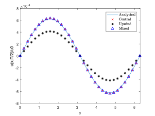
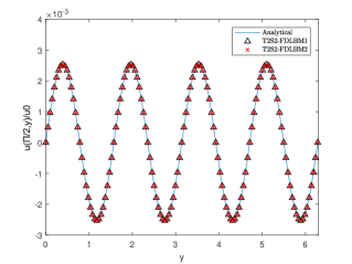
Figure 4: Velocity profiles at $t_{c}=ln[2\nu(k_{1}^{2}+k_{2}^{2})]$ [(a) $u$ along the vertical centerline, (b) $v$ along the horizontal centerline].

Table 1: Errors of FDLBM with three difference schemes.

		T1S2-FDLBM		T2S2-FDLBM1		T1S2-FDLBM		T2S2-FDLBM1
		$E(u)$		$E(u)$		$E(v)$		$E(v)$
up-wind		$0.186$		$0.185$		$0.184$		$0.185$
central		$0.00894$		$0.00883$		$0.00884$		$0.00878$
mixed		$0.00678$		$0.00667$		$0.00666$		$0.00660$

In order to test the accuracies of T2S2-FDLBM1 and T2S2-FDLBM2, different grid sizes ($N_{x}\times N_{y}=16\times 64,32\times 128,48\times 192,64\times 256,80\times 320,96\times 384$) and the global relative error ($GRE$) of velocity at $t=t_{c}$ are considered,

$$E(u)=\frac{\sqrt{\sum_{i,j}|u_{i,j}-u_{i,j}^{\prime}|^{2}}}{\sqrt{\sum_{i,j}|u_{i,j}^{\prime}|^{2}}},$$ (59)

where $u_{ij}$ and $u_{ij}^{\prime}$ are numerical and analytical solutions.

As seen from Table 2, the errors obtained from T1S2-FDLBM, T2S2-FDLBM1 and T2S2-FDLBM2 are almost the same, and all of them have a second-order accuracy in space. This can be explained by the fact that the three models use the same mixed difference scheme ($\eta=0.01$) to deal with the gradient terms.

Table 2: $GRE$s and convergence order of FDLBM with $\Delta t=\pi/640$.

Model		$N_{x}\times N_{y}$		$16\times 64$		$32\times 128$		$48\times 192$		$64\times 256$		$80\times 320$		$96\times 384$
T1S2-		$E(u)$		$1.92\times 10^{-2}$		$6.65\times 10^{-3}$		$3.21\times 10^{-3}$		$1.88\times 10^{-3}$		$1.24\times 10^{-3}$		$9.07\times 10^{-4}$
FDLBM		order		$--$		$1.5326$		$1.7981$		$1.8632$		$1.8437$		$1.7349$
T2S2-		$E(u)$		$1.93\times 10^{-2}$		$6.66\times 10^{-3}$		$3.21\times 10^{-3}$		$1.88\times 10^{-3}$		$1.24\times 10^{-3}$		$8.94\times 10^{-4}$
FDLBM1		order		$--$		$1.5318$		$1.7983$		$1.8691$		$1.8645$		$1.7830$
T2S2-		$E(u)$		$1.93\times 10^{-2}$		$6.78\times 10^{-3}$		$3.32\times 10^{-3}$		$1.98\times 10^{-3}$		$1.34\times 10^{-3}$		$9.83\times 10^{-4}$
FDLBM2		order		$--$		$1.5157$		$1.7566$		$1.7966$		$1.7679$		$1.6841$

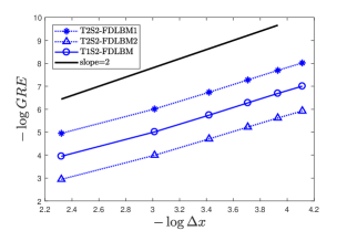
Figure 5: $GRE$ of FDLBM at different gride sizes.

To analyze the stability of the model, we also performed some simulations with different values of $CFL$ condition number. Table 3 shows the $GRE$s of T1S2-FDLBM, T2S2-FDLBM1 and T2S2-FDLBM2. From this table, it can be observed that T1S2-FDLBM is unstable when $CFL$ condition number is more than $0.3$. Compared to T2S2-FDLBM2, T2S2-FDLBM1 works well and maintains a small error even when $CFL=0.9$. These results indicate that the two T2S2-FDLBMs are more stable than the T1S2-FDLBM, and simultaneously, T2S2-FDLBM1 is more suitable to simulate Taylor vortex flow as the $CFL$ condition number increases. It should be noted from the Eq. (50) that $\Delta t$ is proportional to $CFL$ condition number, it means that the value of $CFL$ condition number is related to computational efficiency. For this reason, we further tested the computational efficiency of four methods, i.e., T2S2-FDLBM1, T2S2-FDLBM2, T1S2-FDLBM and SLBM, and presented the results in Table 4. It is found that the CPU time of SLBM, T1S2-FDLBM and T2S2-FDLBM2 are $64$ times, $4.6$ times and $10$ times as long as T2S2-FDLBM1 under the similar error. In this example, one can find that T2S2-FDLBM1 has good stability and high computational efficiency.

Table 3: $GRE$s of FDLBM with different values of $CFL$ condition number.

$CFL$		$0.1$		$0.2$		$0.3$		$0.4$		$0.5$		$0.6$		$0.7$		$0.8$		$0.9$
T1S2-FDLBM $GRE$		$0.0063$		$0.0127$				$-$		$-$		$-$		$-$		$-$		$-$
T2S2-FDLBM1 $GRE$		$0.0064$		$0.0128$		$0.0191$		$0.0255$		$0.0321$		$0.0388$		$0.0460$		$0.0537$		$0.0625$
T2S2-FDLBM2 $GRE$		$0.0058$		$0.0026$		$0.0058$		$0.0161$		$0.0304$		$0.0490$		$0.0727$		$0.1027$		$1.0104$

Table 4: A comparison of four models for the Taylor vortex flow at $t=2t_{c}$.

model		T2S2-FDLBM1			T2S2-FDLBM2			T1S2-FDLBM			SLBM
grid		$32\times 128$	$32\times 128$		$32\times 128$	$32\times 128$		$32\times 128$	$32\times 128$		$512\times 512$	$128\times 128$
$CFL$		$0.8$	$0.9$		$0.1$	$0.6$		$0.1$	$0.2$		–	–
$\Delta t$		$0.0393$	$0.0442$		$0.0049$	$0.0294$		$0.0049$	$0.0098$		$0.0123$	$0.0491$
iterative times		$2076$	$1845$		$16612$	$2768$		$16612$	$8306$		$6645$	$1661$
CPU time		$2.12$	$1.91$		$19.04$	$3.31$		$8.91$	$4.54$		$122.88$	$2.05$
ratio		$1.1099$	$1.0000$		$9.9686$	$1.7330$		$4.6649$	$2.3770$		$64.3351$	$1.0733$
$GRE$ $\times 10^{-2}$		$1.3095$	$1.3228$		$1.1643$	$9.4104$		$1.3412$	$1.3226$		$1.2701$	$4.8907$
ratio		$0.9900$	$1.0000$		$0.8802$	$7.1140$		$1.0139$	$0.9998$		$0.9602$	$3.6972$

B. The two-dimensional Poiseuille flow

Considering the Poiseuille flow driven by a constant external force in a two-dimensional channel, the analytical solution of velocity can be express as

$$u_{x}(y)=4u_{0}\frac{y}{h}\left(1-\frac{y}{H}\right),\quad\quad 0\leq y\leq H,$$ (60)

where $u_{0}=\bar{F}H^{2}/(8\rho_{0}\nu)$ is the maximum velocity, $H$ is the channel height and $\bar{F}$ is the driving force. The Reynolds number $Re=Hu_{0}/\nu$ is related to maximum velocity and pipe height.

In our simulations, $L=H=1.0$ and $Re=10.0$. The periodic boundary condition is used at the inlet and outlet of the channel, and the nonequilibrium extrapolation scheme is applied to treat the nonslip boundary condition at both top and bottom walls, which can be given by

$$\tilde{f}(\bm{x}_{b},\bm{\xi},t)=f_{i}^{eq}(\bm{x}_{b},\bm{\xi}_{i},t)+[\tilde{f}_{i}(\bm{x}_{j},\bm{\xi}_{i},t)-f_{i}^{eq}(\bm{x}_{j},\bm{\xi}_{i},t)].$$ (61)

Initially, the density $\rho=1.0$, $u=v=0.0$, the distribution function is initialized by Eq. (52). For this problem, the non-uniform gird is applied to improve the computational efficiency, which is given by the following transformation,

$$x=\zeta,\quad y=\frac{1}{2a}[a+\tanh(c\mu)],$$ (62)

where $c$ is used to adjust the distribution of the grid and $a=\tanh(c)$. $(\zeta,\mu)$ is the point of grid specified by $\zeta_{i}=i/N_{x}$ and $\mu_{j}=(2j-N_{y})/N_{y}$, where $i=0,1,...,N_{x}$ and $j=0,1,...,N_{y}$. In our simulations, we set $N_{x}\times N_{y}=10\times 20$ and $c=1.5$. Fig. 6 shows the distribution of non-uniform grids. The driving force $\bar{F}$ is chosen to be 0.01 to keep the maximum velocity $u_{0}$ small, the time step can be set as $\Delta t=0.1\times y_{1}$, where $y_{1}$ represents the height from the bottom to the first layer of the grid.

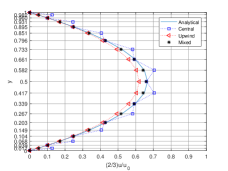
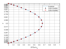
Figure 6: Distributions of non-uniform grids and the velocity along the centerline.

Table 5: Errors for the different difference schemes Poiseuille flow.

		T1S2-FDLBM		T2S2-FDLBM1		T1S2-FDLBM		T2S2-FDLBM1
		center error		center error		$GRE$		$GRE$
up-wind		$3.719\times 10^{-5}$		$3.287\times 10^{-5}$		$4.502\times 10^{-6}$		$1.291\times 10^{-6}$
central		$9.212\times 10^{-6}$		$5.098\times 10^{-6}$		$9.615\times 10^{-6}$		$2.705\times 10^{-6}$
mixed		$4.479\times 10^{-6}$		$2.641\times 10^{-6}$		$5.708\times 10^{-6}$		$2.538\times 10^{-6}$

Table 6: $GRE$s and temporal accuracy orders of FDLBM with non-uniform grid.

Model		$\Delta t$		$0.2\times y1$		$0.3\times y1$		$0.4\times y1$		$0.5\times y1$		$0.6\times y1$		$0.7\times y1$
T1S2-		E(u)		$1.09\times 10^{-5}$		$1.51\times 10^{-5}$		$1.98\times 10^{-5}$		$2.29\times 10^{-5}$		$-$		$-$
FDLBM		order		$--$		$0.8004$		$0.9435$		$0.6549$		$-$		$-$
T2S2-		E(u)		$6.45\times 10^{-6}$		$1.35\times 10^{-5}$		$2.39\times 10^{-5}$		$3.69\times 10^{-5}$		$5.38\times 10^{-5}$		$7.35\times 10^{-5}$
FDLBM1		order		$--$		$1.8235$		$1.9911$		$1.9434$		$2.0640$		$2.0187$
T2S2-		E(u)		$3.34\times 10^{-4}$		$7.62\times 10^{-4}$		$1.38\times 10^{-3}$		$2.20\times 10^{-3}$		$3.23\times 10^{-3}$		$4.52\times 10^{-3}$
FDLBM2		order		$--$		$2.0337$		$2.0587$		$2.0889$		$2.1258$		$2.1696$

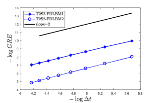
Figure 7: The $GRE$ of T2S2-FDLBM1 with the non-uniform grid at different time steps.

Fig. 6 displays the numerical results of T2S2-FDLBM1 with the up-wind, central and mixed difference scheme ($\eta=0.1$). The results of T2S2-FDLBM1 and T2S2-FDLBM2 are also shown in Fig. 6. From this figure, it can be observed that there are some numerical oscillations in the central difference scheme, and the phenomenon of numerical dissipation appears in the second-order upwind difference scheme. In general, the result of mixed scheme is the most accurate, which is similar to that of the T1S2-FDLBM [1]. However, it should be noted that the numerical oscillation of the central difference scheme in T2S2-FDLBM1 is much smaller than T1S2-FDLBM [1]. This also indicates that T2S2-FDLBM1 is more stable. In addition, as seen from Fig. 6, the results of T2S2-FDLBM1 and T2S2-FDLBM2 with mixed difference scheme agree well with the analytical solution when $CFL=0.1$. The error of velocity at the centerline is given in Table 5. From this table, one can find that the T2S2-FDLBM1 is more accurate than T1S2-FDLBM.

Table 7: $GRE$s of Poiseuille flow with different values of $CFL$ condition number.

$CFL$		$0.1$		$0.2$		$0.3$		$0.4$		$0.5$		$0.6$		$0.7$		$0.8$		$0.9$
T1S2-FDLBM $GRE$$(\times 10^{-4})$		$0.0961$		$0.1092$		$0.1510$		$0.1981$		$0.2293$		$-$		$-$		$-$		$-$
T2S2-FDLBM1 $GRE$$(\times 10^{-4})$		$0.0254$		$0.0645$		$0.1350$		$0.2394$		$0.3693$		$0.5381$		$0.7345$		$0.9582$		$1.2137$
T2S2-FDLBM2 $GRE$$(\times 10^{-4})$		$0.0254$		$3.3396$		$7.6177$		$13.7733$		$21.9519$		$32.3438$		$45.1894$		$60.7891$		$79.5211$

Table 8: A comparison of four different methods for Poiseuille flow at $t=20s$.

model		T2S2-FDLBM1			T2S2-FDLBM2			T1S2-FDLBM			SLBM
grid		$10\times 20$	$10\times 20$		$10\times 20$	$10\times 20$		$10\times 20$	$10\times 20$		$80\times 80$	$20\times 20$
$CFL$		$0.1$	$0.9$		$0.1$	$0.9$		$0.1$	$0.5$		–	–
$\Delta t$		$0.0017$	$0.0155$		$0.0017$	$0.0155$		$0.0017$	$0.0086$		$0.0125$	$0.0500$
iterative times		$11643$	$1293$		$11643$	$1293$		$11643$	$2328$		$1600$	$400$
CPU time		$6.1400$	$0.7500$		$7.6690$	$0.9090$		$3.8590$	$0.7970$		$6.3750$	$0.1720$
ratio		$8.1867$	$1.0000$		$10.2253$	$1.2120$		$5.1453$	$1.0627$		$8.5000$	$0.2293$
$GRE$		$1.3618\times 10^{-5}$	$1.2155\times 10^{-4}$		$8.2600\times 10^{-5}$	$7.9521\times 10^{-3}$		$2.7805\times 10^{-5}$	$1.3623\times 10^{-4}$		$1.7095\times 10^{-4}$	$6.8185\times 10^{-4}$
ratio		$0.1120$	$1.0000$		$0.6796$	$65.4225$		$0.2288$	$1.1208$		$1.4064$	$5.6096$

To test the convergence order of two T2S2-FDLBMs in time, the $GRE$s at different time steps are calculated in Table 6. It can be seen that the T1S2-FDLBM is only first-order accurate in time, while the T2S2-FDLBM1 and T2S2-FDLBM2 have a second-order convergence rate, which is also consistent with the theoretical analysis. In addition, we also tested the effect of $CFL$ condition number, and presented the results in Table 7. From this table, it can be found that the maximum values of $CFL$ condition number in T2S2-FDLBM1 and T2S2-FDLBM2 can reach to 0.9, while it is only about $0.5$ in T1S2-FDLBM. The $GRE$s of T2S2-FDLBM2 are larger than T2S2-FDLBM1 as $CFL$ condition number increases. In Table 8, we presented a comparison of the computational efficiency of four methods. Under the condition of similar error, the CPU time of SLBM is $8.5$ times as long as T2S2-FDLBM. While under the condition of similar CPU time, the $GRE$ of T1S2-FDLBM is a little larger than that of T2S2-FDLBM1, and the $GRE$ of T2S2-FDLBM2 is $65.4$ times as large as T2S2-FDLBM1. Therefore, compared with other three methods, T2S2-FDLBM1 is more efficient.

C. The lid-driven cavity flow

As a classic problem, the lid-driven cavity flow is also used to test T2S2-FDLBM1. The lid-driven cavity flow is driven by a constant velocity of the top wall, and the other three solid walls remain stationary. To obtain accurate results, it is necessary to refine the grid at the four corners, this is because the flow phenomenon at the four corners are very complex [49].

T2S2-FDLBM1 is applied to simulate the lid-driven flow in a square cavity. The height of the square cavity is set to be $1.0$. The top wall moves horizontally from left to right with a constant velocity $u_{0}=0.1$. The initial density and velocity are chosen to be $\rho=1.0$ and $\textbf{u}=\textbf{0}$. The boundary conditions are treated by the non-equilibrium extrapolation scheme. The non-uniform is also applied for this problem,

$$x=\frac{1}{2a}[a+\tanh(c\zeta)],\quad y=\frac{1}{2a}[a+\tanh(c\mu)],$$ (63)

where $c=1.5$ and $a=\tanh(c)$. $(\zeta,\mu)$ is the point of grid set by $\zeta_{i}=i/N_{x}$ and $\mu_{j}=j/N_{y}$, where $i=0,1,...,N_{x}$ and $j=0,1,...,N_{y}$. In our simulations, $N_{x}\times N_{y}=64\times 64$ for $Re=400$ and $1000$, $N_{x}\times N_{y}=128\times 128$ for$Re=3200$ and $5000$, the time step is set to be $\Delta t=0.1\times y_{1}$. In order to eliminate the numerical dissipation, the parameter $\eta$ is set to be 0.1 for $Re=400$ and $1000$, and 0.05 for$Re=3200$ and $5000$. The $GRE$ of lid-driven cavity flow can be defined as

$$\ E(u)=\frac{\sqrt{\sum_{i,j}|u_{i,j}(t_{n})-u_{i,j}(t_{n-1})|^{2}}}{\sqrt{\sum_{i,j}|u_{i,j}(t_{n})|^{2}}}.$$ (64)

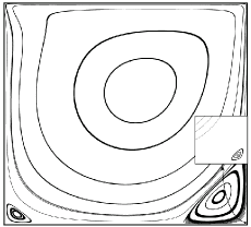
(a) $Re=400$

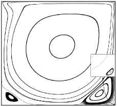
(b) $Re=1000$

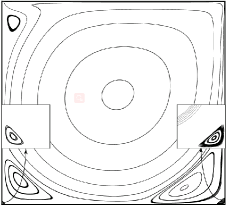
(c) $Re=3200$

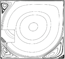
(d) $Re=5000$

Figure 8: Streamlines of lid-driven cavity flow with different Reynolds.

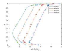
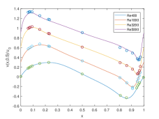
Figure 9: Velocity profiles along the centerline at different $Re$, (o) is reference date. [(a) $Re$=400, 1000, 3200, 5000 from left to right; (b) $Re$=400, 1000, 3200, 5000 from bottom to top.]

Table 9: $GRE$s of lid-driven cavity flow with different values of $CFL$ condition number.

$CFL$		$0.1$		$0.2$		$0.3$		$0.4$		$0.5$		$0.6$		$0.7$		$0.8$		$0.9$
T1S2-FDLBM $GRE$		$0.5816$		$0.4934$		$-$		$-$		$-$		$-$		$-$		$-$		$-$
T2S2-FDLBM1 $GRE$		$0.5725$		$0.4858$		$0.4681$		$0.4609$		$0.4565$		$0.4542$		$0.4524$		$0.4517$		$0.4510$

Table 10: The vortices location of lid-driven cavity flow.

				Primary Vortex			Left Lower Vortex			Right Lower Vortex
				$X$	$Y$		$X$	$Y$		$X$	$Y$
$Re=1000$		SLBM [50]		$0.5313$	$0.5625$		$0.0859$	$0.0781$		$0.8594$	$0.1094$
		T2S2-FDLBM1		$0.5330$	$0.5670$		$0.0850$	$0.0796$		$0.8600$	$0.1136$
$Re=5000$		SLBM [51]		$0.5176$	$0.5373$		$0.0784$	$0.1373$		$0.8078$	$0.0745$
		T2S2-FDLBM1		$0.5162$	$0.5460$		$0.0704$	$0.1442$		$0.7990$	$0.0699$

Fig. 8 shows streamline of the lid-drive flow at different values of Reynolds number. It can be observed that four vortices appear in the cavity when $Re\leq 1000$: a primary vortex at the center of the cavity, a pair of secondary vortices at the lower left and lower right corners, a third level vortex at the lower right corner. When $Re$ is up to $3200$ or $5000$, a third secondary vortex appears in the upper left corner. As $Re$ increases, the center of the primary vortex approaches the center of the cavity. Compared with the results of SLBM [50], T2S2-FDLBM1 can capture more flow details even for $N_{x}\times N_{y}=64\times 64$. Fig. 9 displays the velocity $u$ and $v$ along the centerline of the cavity. It can be found that the results are in good agreement with the previous work [50, 52, 53]. In Table 10, the locations of the vortices are also consistent with the available results [50, 51]. From Tab. 9, it is observed that the range of the $CFL$ condition number in T2S2-FDLBM1 is larger than that in SLBM. Besides, the stability of SLBM, T1S2-FDLBM and T2S2-FDLBM1 are also tested with this example. Under a small grid size ($64\times 64$), the SLBM will be divergent when $Re>8600$, but T1S2-FDLBM and T2S2-FDLBM1 can work well even for $Re\geq 20000$.

4 Conclusions

In this work, a class of T2S2-FDLBM with a second-order accuracy in time and space is proposed based on T1S2-FDLBM presented by Guo et al. [1]. In this method, a simplified TFTD method is applied for time discretization, and a mixed difference scheme is used for space discretization. It is also shown that the T1S2-FDLBM is just a special case of the T2S2-FDLBM. Through the stability analysis, two specific T2S2-FDLBMs are determined. We also performed some simulation to test two T2S2-FDLBMs, and the results are in good agreement with analytical solutions or some previous work. In addition, it is shown that the T2S2-FDLBM1 has a second-order accuracy both in time and space, and the non-uniform grid is also applied to improve computational efficiency. Compared with the SLBM, T1S2-FDLBM and T2S2-FDLBM2, T2S2-FDLBM1 can give more accurate results, and is also more efficient. On the other hand, the CFL condition number in two T2S2-FDLBMs can be changed in a larger range, this feature can be also used to remove the limitation of time step in T1S2-FDLBM. Finally, T2S2-FDLBM1 is more stable, and the numerical oscillations can be reduced effectively. Moreover, T2S2-FDLBM can be also extended to nonlinear convection-diffusion equation, which would be discussed in a future work.

References

References

- [1] Z. Guo, T. Zhao, Explicit finite-difference lattice boltzmann method for curvilinear coordinates, Phys. Rev. E 67 (6) (2003) 066709.
- [2] D. Raabe, Overview of the lattice boltzmann method for nano-and microscale fluid dynamics in materials science and engineering, Model. Simul. Mater. Sci. Eng. 12 (6) (2004) R13.
- [3] Z. Guo, C. Shu, Lattice Boltzmann method and its applications in engineering, Vol. 3, World Scientific, 2013.
- [4] C. Lim, C. Shu, X. Niu, Y. Chew, Application of lattice boltzmann method to simulate microchannel flows, Phys. Fluids 14 (7) (2002) 2299–2308.
- [5] Z. Guo, T. Zhao, Lattice boltzmann model for incompressible flows through porous media, Phys. Rev. E 66 (3) (2002) 036304.
- [6] Z. Chai, H. Liang, R. Du, B. Shi, A lattice boltzmann model for two-phase flow in porous media, SIAM J. Sci. Comput. 41 (4) (2019) B746–B772.
- [7] X. Shan, H. Chen, Lattice boltzmann model for simulating flows with multiple phases and components, Phys. Rev. E 47 (3) (1993) 1815–1819.
- [8] X. Shan, H. Chen, Simulation of nonideal gases and liquid-gas phase transitions by the lattice boltzmann equation, Phys. Rev. E 49 (4) (1994) 2941–2948.
- [9] M. R. Swift, W. R. Osborn, J. M. Yeomans, Lattice boltzmann simulation of nonideal fluids, Phys. Rev. Lett. 75 (5) (1995) 830–833.
- [10] H. Wang, Z. Chai, B. Shi, H. Liang, Comparative study of the lattice boltzmann models for allen-cahn and cahn-hilliard equations, Phys. Rev. E 94 (3) (2016) 033304.
- [11] Z. Chai, D. Sun, H. Wang, B. Shi, A comparative study of local and nonlocal allen-cahn equations with mass conservation, Int. J. Heat Mass Transf. 122 (2018) 631–642.
- [12] H. Wang, X. Yuan, H. Liang, Z. Chai, B. Shi, A brief review of the phase-field-based lattice boltzmann method for multiphase flows, Capillarity 2 (3) (2019) 33–52.
- [13] H. Chen, S. Kandasamy, S. Orszag, R. Shock, S. Succi, V. Yakhot, Extended boltzmann kinetic equation for turbulent flows, Science 301 (5633) (2003) 633–636.
- [14] G. Strumolo, V. Babu, New directions in computational aerodynamics, Phys. World 10 (8) (1997) 45.
- [15] X. He, L. Luo, M. Dembo, Some progress in lattice boltzmann method. part i. nonuniform mesh grids, J. Comput. Phys. 129 (2) (1996) 357–363.
- [16] D. Yu, R. Mei, W. Shyy, A multi-block lattice boltzmann method for viscous fluid flows, Int. J. Numer. Methods Fluids 39 (2) (2002) 99–120.
- [17] O. Filippova, D. Hänel, Grid refinement for lattice-bgk models, J. Comput. Phys. 147 (1) (1998) 219–228.
- [18] C. Lin, Y. Lai, Lattice boltzmann method on composite grids, Phys. Rev. E 62 (2) (2000) 2219.
- [19] D. Lagrava, O. Malaspinas, J. Latt, B. Chopard, Advances in multi-domain lattice boltzmann grid refinement, J. Comput. Phys. 231 (14) (2012) 4808–4822.
- [20] B. Crouse, E. Rank, M. Krafczyk, J. Tölke, A lb-based approach for adaptive flow simulations, Int. J. Mod. Phys. B 17 (01n02) (2003) 109–112.
- [21] J. Tölke, S. Freudiger, M. Krafczyk, An adaptive scheme using hierarchical grids for lattice boltzmann multi-phase flow simulations, Comput. fluids 35 (8-9) (2006) 820–830.
- [22] J. Wu, C. Shu, A solution-adaptive lattice boltzmann method for two-dimensional incompressible viscous flows, J. Comput. Phys. 230 (6) (2011) 2246–2269.
- [23] Y. Chen, Q. Kang, Q. Cai, D. Zhang, Lattice boltzmann method on quadtree grids, Phys. Rev. E 83 (2) (2011) 026707.
- [24] A. Fakhari, T. Lee, Finite-difference lattice boltzmann method with a block-structured adaptive-mesh-refinement technique, Phys. Rev. E 89 (3) (2014) 033310.
- [25] H. Wang, B. Shi, H. Liang, Z. Chai, Finite-difference lattice boltzmann model for nonlinear convection-diffusion equations, Appl. Math. Comput. 309 (2017) 334–349.
- [26] X. Guo, B. Shi, Z. Chai, General propagation lattice boltzmann model for nonlinear advection-diffusion equations, Phys. Rev. E 97 (4) (2018) 043310.
- [27] T. Lee, C.-L. Lin, An eulerian description of the streaming process in the lattice boltzmann equation, J. Comput. Phys. 185 (2) (2003) 445–471.
- [28] G. Eitel Amor, M. Meinke, W. Schröder, A lattice-boltzmann method with hierarchically refined meshes, Comput. Fluids 75 (2013) 127–139.
- [29] Z. Guo, K. Xu, R. Wang, Discrete unified gas kinetic scheme for all knudsen number flows: Low-speed isothermal case, Phys. Rev. E 88 (2013) 033305.
- [30] C. Wu, B. Shi, Z. Chai, P. Wang, Discrete unified gas kinetic scheme with a force term for incompressible fluid flows, Comput. Math. Appl. 71 (12) (2016) 2608–2629.
- [31] T. Lee, C. Lin, A characteristic galerkin method for discrete boltzmann equation, J. Comput. Phys. 171 (1) (2001) 336–356.
- [32] M. B. Reider, J. D. Sterling, Accuracy of discrete-velocity bgk models for the simulation of the incompressible navier-stokes equations, Comput. fluids 24 (4) (1995) 459–467.
- [33] N. Cao, S. Chen, S. Jin, D. Martinez, Physical symmetry and lattice symmetry in the lattice boltzmann method, Phys. Rev. E 55 (1) (1997) R21.
- [34] R. Mei, W. Shyy, On the finite difference-based lattice boltzmann method in curvilinear coordinates, J. Comput. Phys. 143 (2) (1998) 426–448.
- [35] Z. Guo, T. Zhao, Finite-difference-based lattice boltzmann model for dense binary mixtures, Phys. Rev. E 71 (2) (2005) 026701.
- [36] Y. Wang, Y. He, J. Huang, Q. Li, Implicit–explicit finite-difference lattice boltzmann method with viscid compressible model for gas oscillating patterns in a resonator, Int. J. Numer. Methods Fluids 59 (8) (2009) 853–872.
- [37] M. El-Amin, S. Sun, A. Salama, On the stability of the finite difference based lattice boltzmann method, Proc. Comput. Sci. 18 (2013) 2101–2108.
- [38] L. Kim, H. Yang, M. Ha, Z. Xu, H. Xiao, S. Lyu, Immersed boundary-finite difference lattice boltzmann method using the feedback forcing scheme to simulate the incompressible flows, Int. J. Precis. Eng. Manuf. 17 (8) (2016) 1049–1057.
- [39] M. Watari, Velocity slip and temperature jump simulations by the three-dimensional thermal finite-difference lattice boltzmann method, Phys. Rev. E 79 (6) (2009) 066706.
- [40] E. Ezzatneshan, K. Hejranfar, Simulation of three-dimensional incompressible flows in generalized curvilinear coordinates using a high-order compact finite-difference lattice boltzmann method, Int. J. Numer. Methods Fluids 89 (7) (2019) 235–255.
- [41] K. Hejranfar, E. Ezzatneshan, A high-order compact finite-difference lattice boltzmann method for simulation of steady and unsteady incompressible flows, Int. J. Numer. Methods Fluids 75 (10) (2014) 713–746.
- [42] K. Hejranfar, E. Ezzatneshan, Simulation of two-phase liquid-vapor flows using a high-order compact finite-difference lattice boltzmann method, Phys. Rev. E 92 (5) (2015) 053305.
- [43] K. Hejranfar, M. H. Saadat, Preconditioned weno finite-difference lattice boltzmann method for simulation of incompressible turbulent flows, Comput. Math. Appl. 76 (6) (2018) 1427–1446.
- [44] C. Wu, B. Shi, C. Shu, Z. Chai, Third-order discrete unified gas kinetic scheme for continuum and rarefied flows: Low-speed isothermal case, Phys. Rev. E 97 (2) (2018) 023306.
- [45] J. Li, Z. Du, A two-stage fourth order time-accurate discretization for lax–wendroff type flow solvers i. hyperbolic conservation laws, SIAM J. Sci. Comput. 38 (5) (2016) A3046–A3069.
- [46] Z. Guo, K. Xu, R. Wang, Discrete unified gas kinetic scheme for all knudsen number flows: Low-speed isothermal case, Phys. Rev. E 88 (3) (2013) 033305.
- [47] X. He, L. Luo, Lattice boltzmann model for the incompressible navier–stokes equation, J. Stat. Phys 88 (3-4) (1997) 927–944.
- [48] Z. Guo, C. Zheng, B. Shi, Discrete lattice effects on the forcing term in the lattice boltzmann method, Phys. Rev. E 65 (4) (2002) 046308.
- [49] Z. Chai, B. Shi, L. Zhen, Simulating high reynolds number flow in two-dimensional lid-driven cavity by multi-relaxation-time lattice boltzmann method, Chinese Phys. 15 (8) (2006) 1855–1863.
- [50] U. Ghia, K. N. Ghia, C. Shin, High-re solutions for incompressible flow using the navier-stokes equations and a multigrid method, J. Comput. Phys. 48 (3) (1982) 387–411.
- [51] S. Hou, Q. Zou, S. Chen, G. Doolen, A. C. Cogley, Simulation of cavity flow by the lattice boltzmann method, J. Comput. Phys. 118 (2) (1995) 329–347.
- [52] R. Schreiber, H. B. Keller, Driven cavity flows by efficient numerical techniques, J. Comput. Phys. 49 (2) (1983) 310–333.
- [53] S. P. Vanka, Block-implicit multigrid solution of navier-stokes equations in primitive variables, J. Comput. Phys. 65 (1) (1986) 138–158.