Data processing over single-port homodyne detection to realize super-resolution and super-sensitivity

Abstract

Performing homodyne detection at one port of squeezed-state light interferometer and then binarzing measurement data are important to achieve super-resolving and super-sensitive phase measurements. Here we propose a new data-processing technique by dividing the measurement quadrature into three bins (equivalent to a multi-outcome measurement), which leads to a higher improvement in the phase resolution and the phase sensitivity under realistic experimental condition. Furthermore, we develop a new phase-estimation protocol based on a combination of the inversion estimators of each outcome and show that the estimator can saturate the Cramér-Rao lower bound, similar to asymptotically unbiased maximum likelihood estimator.

I Introduction

Optimal measurement scheme followed by a proper data processing is important to realize high-precision and high-resolution phase measurements RMP ; Ma ; Dowling2008 . For the commonly used intensity measurement over quasi-classical coherent states, the achievable phase sensitivity is subject to the shot-noise limit (SNL) $\delta\theta\sim O(1/\sqrt{\bar{n}})$, where $\bar{n}$ is the number of particles of the input state. Furthermore, the intensity measurement at the output-port of the coherent-state light interferometer gives rise to an oscillatory interferometric signal $\propto\sin^{2}(\theta/2)$ or $\cos^{2}(\theta/2)$, which exhibits the fringe resolution $\lambda/2$ determined by wavelength of the incident light $\lambda$. This is often referred to the classical resolution limit of interferometer, or the Rayleigh resolution criterion in optical imaging Boto . These two classical limits in the sensitivity and the resolution can be surpassed with non-classical states of the light Giovannetti2004 ; Durkin2007 such as the $N$-photon NOON state $(|N,0\rangle_{a,b}+|0,N\rangle_{a,b})/\sqrt{2}$. This is a maximally entangled state with all the particles being either in the mode $a$ or all in the mode $b$, leading to the super-sensitivity $\delta\theta\sim O(1/N)$ and the super-resolution $\lambda/(2N)$ Dowling2008 ; Boto ; Giovannetti2004 ; Durkin2007 ; Gerry2003 . However, the NOON states are difficult to prepare and are fragile to the loss-induced decoherence Braun ; Dorner ; Zhang2013a .

Recently, several important progresses have been reported. The first one is the achievement of super-resolution by feeding the interferometer with a coherent laser, followed by coincidence photon counting Resch , parity detection Gao ; Cohen , and homodyne detection with a proper data processing Distante . Specially, Distante et al Distante detect the field quadrature at one port of coherent-state light interferometer and then binarize the measurement data $p\in(-\infty,+\infty)$ into two bins $p\in[-a,a]$ and $p\notin[-a,a]$, which results in a deterministic and robust super-resolution with classical states of the light. The second progress is the recent theoretical proposal and experimental demonstration Schafermeier that feeding a coherent state and a squeezed vacuum state into the two input ports of the interferometer followed by the same data processing over the single-port homodyne detection, which can realize deterministic super-resolution and super-sensitivity simultaneously with Gaussian states of light and Gaussian measurements Schafermeier . This result may provide a powerful and efficient way to enhance the sensitivity of gravitational wave detectors LIGO1 ; LIGO2 and that of correlation interferometry Pradyumna .

The data-processing method proposed by Refs. Distante ; Schafermeier is equivalent to a binary-outcome measurement Feng ; Ghirardi ; Jin , where the outcome “$0$” corresponds to $p\in[-a,a]$ and the outcome “$\emptyset$” for $p\notin[-a,a]$. To infer an unknown phase shift, the simplest protocol of the phase estimation has been used by inverting the averaged signal Distante ; Schafermeier . The advantage of the inversion estimator is that it has a relatively simple analytical expression and its sensitivity follows the simple error-propagation formula Distante ; Schafermeier . Moreover, for any binary-outcome measurement, it has been shown that the inversion estimator asymptotically saturates the Cramér-Rao lower bound (CRB) Feng ; Ghirardi ; Jin . However, the binarization of measurement data and the inversion estimator suffer from a serious drawback, i.e., they do not take into account all the information from the measurement YMK ; Pezze . Consequently, they tend to degrade the achievable sensitivity significantly, e.g., at $\theta=0$, the sensitivity diverges Distante ; Schafermeier , so the inversion estimator cannot infer the true value of phase shift in the vicinity $\theta\sim 0$.

In this paper, we propose a new strategy capable of further improving both the resolution and the sensitivity using the experimental setup similar to Schafermeier et al Schafermeier . Our strategy consists of two essential ingredients. The first one is to divide the measurement data into three bins: $(-\infty,-a)$, $[-a,a]$, and $(a,\infty)$, corresponding to three outcomes “$-$”, “0”, and “$+$” , respectively. This is equivalent to a three-outcome measurement and enjoys two advantages over the previous binary-outcome case Schafermeier : (i) The divergence of phase sensitivity at $\theta=0$ is removed, which is useful for estimating a small phase shift; (ii) Higher improvement in the resolution and the sensitivity is achievable under realistic experimental parameters. The second ingredient is a composite estimator based on a linear combination of the inversion estimators associated with each measurement outcome. This estimator takes into account available information from all the measurement outcomes of a general multi-outcome measurement, so it is capable of saturating the CRB asymptotically. Therefore, this composite estimator enjoys the good merits of the inversion estimator (i.e., the simplicity) and the well-known maximum-likelihood estimator (i.e., unbiasedness and asymptotic optimality in the sensitivity). In addition to the squeezed-state light inteferometry, our estimation protocol may also be applicable to other kinds of multi-outcome measurements.

II Single-port Homodyne detection without data-processing

As depicted by Fig. 1(a), we consider the homodyne detection at one port of the interferometer that fed by a coherent state $|\alpha_{0}\rangle$ and a squeezed vacuum $|\xi_{0}\rangle$ (i.e., the so-called squeezed-state interferometer) Caves ; Pezze2008 . To enlarge available information about the phase shift $\theta$, the field amplitudes are chosen as $\alpha_{0}\in\mathbb{R}$ and $\xi_{0}=-r\in\mathbb{R}$ (i.e., $\arg\alpha_{0}=0$ and $\arg\xi_{0}=\pi$); See Refs. LJing ; LPan1 ; LPan2 and also the Appendix. The total number of photons injected from the two input ports is given by $\bar{n}=\alpha_{0}^{2}+\sinh^{2}r$. Furthermore, the Wigner function of the input state is given by Gerrybook

$$W_{\mathrm{in}}(\alpha,\beta) = W_{|\alpha_{0}\rangle}(\alpha)W_{|\xi_{0}\rangle}(\beta)$$ (1)

$$= \frac{2}{\pi}e^{-2\left[\left(x_{a}-\alpha_{0}\right)^{2}+p_{a}^{2}\right]}\cdot\frac{2\sqrt{\tilde{\mu}\tilde{\nu}}}{\pi}e^{-2\left(\tilde{\mu}x_{b}^{2}+\tilde{\nu}p_{b}^{2}\right)},$$

where $\alpha=x_{a}+ip_{a}$, $\beta=x_{b}+ip_{b}$, and

$$\tilde{\mu}=\varrho^{2}e^{-2r},\text{ \ \ \ \ }\tilde{\nu}=e^{2r},$$ (2)

with $\varrho$ ($\leq 1$) and $e^{-r}$ describing the purity and the squeeze parameter of $|\xi_{0}\rangle$. The Wigner function of the output state takes the same form with the input state $W_{\mathrm{out}}(\alpha,\beta;\theta)=W_{\mathrm{in}}(\tilde{\alpha}_{\theta},\tilde{\beta}_{\theta})$ Seshadreesan2 ; Tan ; Wang , where the variables $(\alpha,\beta)$ have been replaced by $(\tilde{\alpha}_{\theta},\tilde{\beta}_{\theta})$; see the Appendix. Integrating the Wigner function over $\{x_{a}$, $x_{b}$, $p_{b}\}$, we obtain the conditional probability for detecting a measurement quadrature $p\in(-\infty,\infty)$,

$$P(p|\theta)=\sqrt{\frac{2}{\pi\eta_{\theta}}}\exp\left[-\frac{2}{\eta_{\theta}}\left(p+\frac{\alpha_{0}}{2}\sin\theta\right)^{2}\right],$$ (3)

where, for brevity, we omit the subscript “$a$” in the quadrature $p_{a}$, and introduce

$$\eta_{\theta}=\frac{\tilde{\mu}+\tilde{\nu}+2\tilde{\mu}\tilde{\nu}-2\tilde{\mu}(\tilde{\nu}-1)\cos\theta+(\tilde{\mu}-\tilde{\nu})\cos^{2}\theta}{4\tilde{\mu}\tilde{\nu}}.$$ (4)

Note that Eq. (3) holds for the homodyne detection at one port of the interferometer fed by the input $|\alpha_{0}\rangle\otimes|\xi\rangle$. Here $|\xi\rangle$ could be arbitrary gaussian state of light, with $\tilde{\mu}$ and $\tilde{\nu}$ to be determined by $|\xi\rangle$. As the simplest case, the coherent-state input $|\alpha_{0}\rangle\otimes|0\rangle$ corresponds to $\tilde{\mu}=\tilde{\nu}=\varrho=1$ and hence $\eta_{\theta}=1$, in agreement with our previous result Feng .

In Fig. 1(b), we show density plot of $P(p|\theta)$ against the phase shift $\theta$ and the measurement quadrature $p$, where the red dashed line is given by $p=-\alpha_{0}\sin(\theta)/2$. This equation takes the same form with that of the signal

$$\langle\hat{p}(\theta)\rangle=\int_{-\infty}^{\infty}P(p|\theta)pdp=-\frac{\alpha_{0}}{2}\sin\theta,$$ (5)

which shows the full width at half maximum ($\mathrm{FWHM}$) $=2\pi/3$, and hence the Rayleigh limit in fringe resolution Distante ; Schafermeier .

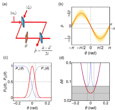
Figure 1: (a) Homodyne detection (i.e., measuring the quadrature operator $\hat{p}$) at one port of the interferometer that fed by a coherent state $|\alpha_{0}\rangle$ and a squeezed vacuum $|\xi_{0}\rangle$. (b) Density plot of the probability $P(p|\theta)$ against the phase shift $\theta$ and the measurement quadrature $p$, given by Eq. (3). (c) Occurrence probabilities $P_{-}(\theta)$, $P_{0}(\theta)$, and $P_{+}(\theta)$ for detecting $p\in(-\infty,-a)$, $[-a,a]$, and $(a,\infty)$. This data-processing method is equivalent to a multi-outcome measurement. (d) The CRB of the phase sensitivity for the multi-outcome measurement $\delta\theta_{\mathrm{mul}}$ (red solid line), better than that of a binary-outcome measurement $\delta\theta_{\mathrm{bin}}$ (blue dashed line), where the measured data is divided into only two bins Schafermeier : $p\in[-a,a]$ and $p\notin[-a,a]$. Vertical lines in (c) and (d): the $\mathrm{FWHM}$ of the scaled $P_{0}(\theta)$ and the best sensitivity of the binary-outcome measurement $\delta\theta_{\mathrm{bin},\min}=\delta\theta_{\mathrm{bin}}(\theta_{\min})$. The shaded area in (d): the region for the sensitivity better than the SNL $1/\sqrt{\bar{n}}$, where $\bar{n}=200$ (with $\alpha_{0}^{2}=199.3$) and the bin size $a=0.1$.

According to Refs. Helstrom ; Braunstein1 ; Braunstein2 ; Paris2009 , the ultimate phase estimation precision is determined by the CFI:

$$\mathcal{F}(\theta) = \int_{-\infty}^{\infty}\frac{[P^{\prime}(p|\theta)]^{2}}{P(p|\theta)}dp$$ (6)

$$= \frac{(\alpha_{0}\cos\theta)^{2}}{\eta_{\theta}}+\frac{\left[\tilde{\mu}-\tilde{\mu}\tilde{\nu}+(\tilde{\mu}-\tilde{\nu})\cos\theta\right]^{2}\sin^{2}\theta}{8(\tilde{\mu}\tilde{\nu}\eta_{\theta})^{2}},$$

where $P^{\prime}\equiv\partial P/\partial\theta$. When the coherent-state component dominates over the squeezed vacuum, maximum of the CFI occurs at $\theta=0$, i.e., $\mathcal{F}(0)=\alpha_{0}^{2}/\eta_{0}=\tilde{\nu}\alpha_{0}^{2}\simeq e^{2r}\bar{n}$, which yields a sub-shot-noise sensitivity:

$$\delta\theta_{\mathrm{CRB},\mathrm{\min}}=\frac{1}{\sqrt{\mathcal{F}(0)}}\simeq\frac{e^{-r}}{\sqrt{\bar{n}}}.$$ (7)

This is the best sensitivity attained from the single-port homodyne detection in the limit $\alpha_{0}^{2}\gg\sinh^{2}r$, coincident with the intensity-difference measurement Caves ; Pezze2008 .

III Binary-outcome homodyne detection

To improve the resolution, one can separate the measured data into two bins Distante : $p\in[-a,a]$ as an outcome, denoted by “$0$”, and $p\notin[-a,a]$ as an another outcome “$\emptyset$”, with the bin size $2a$. Using Eq. (3), it is easy to obtain the conditional probabilities of the outcomes,

$$P_{0}(\theta)=\int_{-a}^{+a}dpP(p|\theta)=\frac{1}{2}\mathrm{Erf}\left[g_{-}(\theta),g_{+}(\theta)\right],$$ (8)

and hence $P_{\emptyset}(\theta)=1-P_{0}(\theta)$. Here, $\mathrm{Erf}[x,y]=\mathrm{erf}(y)-\mathrm{erf}(x)$ denotes a generalized error function, and

$$g_{\pm}(\theta)=\sqrt{\frac{2}{\eta_{\theta}}}\left(\frac{\alpha_{0}}{2}\sin\theta\pm a\right),$$ (9)

with $\eta_{\theta}$ being defined in Eq. (4). The above data-processing method is equivalent to a binary-outcome measurement Wang , with the observable $\hat{\Pi}=\mu_{0}\hat{\Pi}_{0}+\mu_{\emptyset}\hat{\Pi}_{\emptyset}$, where $\hat{\Pi}_{0}=\int_{-a}^{+a}|p\rangle\langle p|dp$ and $\hat{\Pi}_{\emptyset}=\hat{1}-\hat{\Pi}_{0}$. Obviously, the output signal is given by

$$\langle\hat{\Pi}(\theta)\rangle=\mu_{0}P_{0}(\theta)+\mu_{\emptyset}P_{\emptyset}(\theta),$$ (10)

where we have used the relation $\langle\hat{\Pi}_{k}(\theta)\rangle=P_{k}(\theta)$ for $k=0$ and $\emptyset$. Following Schafermeier et al Schafermeier , in Fig. 1(c), we choose the eigenvalues $\mu_{\emptyset}=0$ and $\mu_{0}=1/\mathrm{erf}(\sqrt{2}ae^{r})$ to show the signal as a function of $\theta$ (see the red solid line), which shows $\langle\hat{\Pi}(0)\rangle=1$. This treatment is useful to determine the $\mathrm{FWHM}$ of the signal and hence the resolution, as depicted by the vertical lines of Fig. 1(c).

In Fig. 2(a), we show numerical results of the $\mathrm{FWHM}$ as functions of the bin size $a$ and the squeezing parameter $e^{-r}$. Similar to Ref. Schafermeier , one can note that the improvement of the $\mathrm{FWHM}$ compared to the Rayleigh criterion $2\pi/3$ (i.e., the ratio $\frac{2\pi/3}{\mathrm{FWHM}}$) increases as $a\rightarrow 0$ and $r\rightarrow\infty$. For a given and finite number of photons $\bar{n}$, this means that a better resolution beyond the Rayleigh criterion (i.e., the super-resolution) can be obtained when $a$, $\alpha_{0}\rightarrow 0$.

Independent on $\mu_{0}$ and $\mu_{\emptyset}$, the phase sensitivity of the binary-outcome measurement is given by

$$\delta\theta_{\mathrm{bin}}=\frac{\Delta\hat{\Pi}}{|\partial\langle\hat{\Pi}(\theta)\rangle/\partial\theta|}=\frac{\sqrt{P_{0}(\theta)P_{\emptyset}(\theta)}}{\left|P_{0}^{\prime}(\theta)\right|},$$ (11)

where $\Delta\hat{\Pi}=\sqrt{\langle\hat{\Pi}^{2}\rangle-\langle\hat{\Pi}\rangle^{2}}$ and $P_{0}^{\prime}=\partial P_{0}/\partial\theta$. On the other hand, the CFI of this binary-outcome measurement is given by Feng

$$\mathcal{F}_{\mathrm{bin}}(\theta)=\sum_{k=0,\emptyset}\frac{\left[P_{k}^{\prime}(\theta)\right]^{2}}{P_{k}(\theta)}=\frac{1}{(\delta\theta_{\mathrm{bin}})^{2}},$$ (12)

where, in the last step, we have used the normalization relation $P_{0}(\theta)+P_{\emptyset}(\theta)=1$. The above results indicate that the phase uncertainty predicted by the error-propagation $\delta\theta_{\mathrm{bin}}$ always saturates the CRB $1/\sqrt{\mathcal{F}_{\mathrm{bin}}(\theta)}$, which holds for any binary-outcome measurement Feng ; Ghirardi ; Jin . As illustrated by the blue dashed line of Fig. 1(d), one can see that the sensitivity reaches its maximum at the optimal working point $\theta_{\min}$ (the vertical lines) and the best sensitivity $\delta\theta_{\mathrm{bin,\min}}\equiv\delta\theta_{\mathrm{bin}}(\theta_{\min})$ can beat the SNL ($=1/\sqrt{\bar{n}}$).

Similar to Ref. Schafermeier , in Fig. 2(b), we show the improvement in the sensitivity $\delta\theta_{\mathrm{bin,\min}}/\mathrm{SNL}$ as functions of the bin size $a$ and the squeezing parameter $e^{-r}$. For a given $\bar{n}=100$, the best sensitivity can reach $4\mathrm{dB}$ when $a=0.5$ and $e^{-r}=0.2$ (i.e., $\sinh^{2}r/\bar{n}\approx 0.06$). From the squares of Fig. 3, one can also find that the $\mathrm{FWHM}$ scales as $(2\pi/3)/\sqrt{\bar{n}}$ and the best sensitivity $\delta\theta_{\mathrm{bin,\min}}\sim 0.75/\bar{n}^{0.54}$, with the scaling better than the $\mathrm{SNL}$ (i.e., the super-sensitivity). Specially, a $22$-fold improvement in the phase resolution and a $1.7$-fold improvement in the sensitivity can be obtained with $a=0.5$, $\alpha_{0}^{2}=427$, and $\sinh^{2}r=0.687$ (i.e., $e^{-r}=0.47$) Schafermeier .

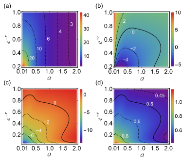
Figure 2: For the purity of the squeezed vacuum $\varrho=0.5$ and given number of photons $\bar{n}=\alpha_{0}^{2}+\sinh^{2}r=100$, density plot of the improvement factor in the resolution $\frac{2\pi/3}{\mathrm{FWHM}}$ (a) against the bin size $a$ and the squeeze parameter $e^{-r}$, and that of the best sensitivities (in units of $\mathrm{dB}$), obtained from the binary-outcome measurement $\delta\theta_{\mathrm{bin},\min}$ (b) and the multi-outcome measurement $\delta\theta_{\mathrm{mul},\min}$ (c). (d) The scaling of the sensitivity $\frac{-\log\delta\theta_{\mathrm{mul},\min}}{\log\bar{n}}$ ($=0.5$ for the shot-noise limit, and $1$ for the Heisenberg limit). The solid lines in (b)-(d): the shot-noise limit.

Normally, the data processing over the measurement quadrature $p\in(-\infty,\infty)$ can increase the resolution, at the cost of reduced phase sensitivity. In this sense, the ultimate phase sensitivity obtained from the single-port homodyne measurement without any data-processing (i.e., $\delta\theta_{\mathrm{CRB},\mathrm{\min}}$) is the best sensitivity of the binary-outcome measurement in the limit $a\rightarrow\infty$ Schafermeier . From Fig. 3, one can see $\delta\theta_{\mathrm{bin,\min}}>\delta\theta_{\mathrm{CRB}\text{,}\mathrm{\min}}$ (the thick solid line). More importantly, $\delta\theta_{\mathrm{bin}}$ diverges at $\theta=0$ and therefore no phase information can be inferred for a small phase shift $\theta\sim 0$. To avoid this problem, we present a new data-processing technique (equivalent to a multi-outcome measurement), based upon the experimental setup similar to Schafermeier et al Schafermeier .

IV Multi-outcome homodyne detection

We now consider a new data-processing method by treating the measurement quadrature $p\in(a,\infty)$ as an outcome, denoted hereinafter by “$+$”, and similarly $p\in(-\infty,-a)$ as an outcome “$-$”. The conditional probabilities for detecting “$\pm$” are given by

$$P_{+}(\theta) = \int_{a}^{\infty}dpP(p|\theta)=\frac{1-\mathrm{erf}[g_{+}(\theta)]}{2},$$ (13)

$$P_{-}(\theta) = \int_{-\infty}^{-a}dpP(p|\theta)=\frac{1+\mathrm{erf}[g_{-}(\theta)]}{2},$$ (14)

which obey the normalization condition $P_{+}(\theta)+P_{0}(\theta)+P_{-}(\theta)=1$ and $g_{\pm}(\theta)$ have been defined in Eq. (9). This is indeed a multi-outcome measurement with the observable $\hat{\Pi}=\sum_{k}\mu_{k}\hat{\Pi}_{k}$ Wang , defined by the projections $\hat{\Pi}_{+}=\int_{a}^{\infty}|p\rangle\langle p|dp$, $\hat{\Pi}_{-}=\int_{-\infty}^{-a}|p\rangle\langle p|dp$, and $\hat{\Pi}_{0}$. In Fig. 1(c), we show $P_{0}$ and $P_{\pm}$ as functions of $\theta$, for $\bar{n}=200$, $a=0.1$, and the purity $\varrho=1$. Hereinafter, we choose a relatively small value of $a$ than that of Ref. Schafermeier to obtain a better resolution and an enhanced sensitivity [see below Figs. 2(c) and (d)].

For a general multi-outcome measurement, the averaged signal can be obtained by taking expectation value of $\hat{\Pi}$ with respect to a phase-encoded state $\hat{\rho}(\theta)$, namely

$$\langle\hat{\Pi}(\theta)\rangle=\sum_{k}\mu_{k}P_{k}(\theta)\approx\sum_{k}\mu_{k}\frac{{\mathcal{N}}_{k}}{{\mathcal{N}}},$$ (15)

where $\mu_{k}$ and $P_{k}(\theta)=\langle\hat{\Pi}_{k}\rangle=\mathrm{Tr}[\hat{\rho}(\theta)\hat{\Pi}_{k}]$ denote the eigenvalue and the conditional probability associated with the $k$th outcome. With ${\mathcal{N}}$ independent measurements, one records the occurrence number of each outcome ${\mathcal{N}}_{k}$ at given $\theta\in(-\pi,\pi)$. As ${\mathcal{N}}\gg 1$, the conditional probabilities can be measured by the occurrence frequencies, due to $P_{k}(\theta)\approx{\mathcal{N}}_{k}/{\mathcal{N}}$. For the multi-outcome homodyne measurement, we numerical simulate $P_{0}(\theta)$ and $P_{\pm}(\theta)$ using $M$ replicas of ${\mathcal{N}}$ random numbers Wang . As illustrated by the solid circles of Fig. 4(a) and (b), one can note that statistical average of the occurrence frequencies ${\mathcal{N}}_{0}/{\mathcal{N}}$ and ${\mathcal{N}}_{\pm}/{\mathcal{N}}$, fitted as $P_{0}^{\mathrm{(fit)}}(\theta)$ and $P_{\pm}^{\mathrm{(fit)}}(\theta)$, show good agreement with their analytical results.

Once all phase-dependent $\{P_{k}(\theta)\}$ and hence $\langle\hat{\Pi}(\theta)\rangle$ are known, one can infer $\theta$ via the inversion estimator $\theta_{\mathrm{inv}}=g^{-1}(\sum_{k}\mu_{k}{\mathcal{N}}_{k}/{\mathcal{N}})$, where $g^{-1}$ denotes the inverse function of $g(\theta)=\langle\hat{\Pi}(\theta)\rangle$. This protocol of phase estimation is commonly used in experiments, since its performance simply follows the error-propagation formula. However, the inversion estimator based on the averaged signal does not take into account all of the available information, especially the fluctuations in the measurement observable at the output ports YMK . To improve the phase information, one can adopt data-processing techniques such as maximal likelihood estimation or Bayesian estimation Pezze , which saturates the CRB Helstrom ; Braunstein1 ; Braunstein2 ; Paris2009 :

$$\Delta\theta_{\mathrm{mul}}=\frac{1}{\sqrt{{\mathcal{N}}\mathcal{F}_{\mathrm{mul}}(\theta)}},$$ (16)

where $\mathcal{F}_{\mathrm{mul}}(\theta)=\sum_{k}f_{k}(\theta)$, being a sum of the CFI of each outcome, with

$$f_{k}(\theta)=\frac{1}{P_{k}(\theta)}\left[\frac{\partial P_{k}(\theta)}{\partial\theta}\right]^{2}.$$ (17)

The phase-dependent $\{P_{k}(\theta)\}$ and hence $\{f_{k}(\theta)\}$ can be obtained in principle, at least, from the interferometric calibration, where the value of $\theta$ is known and tunable.

In Fig. 1(d), we show the sensitivity per measurement $\delta\theta_{\mathrm{mul}}\equiv\sqrt{\mathcal{N}}\Delta\theta_{\mathrm{mul}}$ as a function of $\theta$ (the red line). The best sensitivity occurs at $\theta=0$ and hence $\delta\theta_{\mathrm{mul}\text{,}\min}\equiv 1/\sqrt{\mathcal{F}_{\mathrm{mul}}(0)}$. The improvement of $\delta\theta_{\mathrm{mul}\text{,}\min}$ compared with the $\mathrm{SNL}$ is depicted in Fig. 2(c), which shows larger quantum-enhancement region than that of $\delta\theta_{\mathrm{bin}\text{,}\min}$. In Fig. 2(d), we show the scaling of the best sensitivity $\frac{-\log\delta\theta_{\mathrm{mul}\text{,}\min}}{\log\bar{n}}$ against the bin size $a$ and the squeezing parameter $e^{-r}$, where the solid line implies the $\mathrm{SNL}$. For a given $\bar{n}\gg 1$, one can find that the scaling can even reach the Heisenberg limit as $\alpha_{0}$, $a\rightarrow 0$.

In Fig. 3, we show the scaling of $\delta\theta_{\mathrm{mul}\text{,}\min}$ and compare it with $\delta\theta_{\mathrm{bin}\text{,}\min}$, using the parameters $\sinh^{2}r=0.687$ and $\varrho=0.58$. To optimize the performance, we choose the bin size $a=0.1$ for the multi-outcome measurement; While for the binary-outcome case, we take $a=0.5$ Schafermeier . One can find that numerical results of $\delta\theta_{\mathrm{mul}\text{,}\min}$ (the solid circles) can be well fitted as $1.1e^{-r}/\sqrt{\bar{n}}$, better than that of $\delta\theta_{\mathrm{bin}\text{,}\min}$ (the squares). This result almost approaches the best sensitivity of the single-port homodyne measurement without any data-processing (the thick line). From the inset, one can also note that the signal becomes further narrowing in a comparison with that of Ref. Schafermeier . For instance, a $38$-fold improvement in the resolution and a $1.9$-fold improvement in the sensitivity is achievable with the realistic experimental parameters Schafermeier : $a=0.1$, $\alpha_{0}^{2}=427$, and $\sinh^{2}r=0.687$.

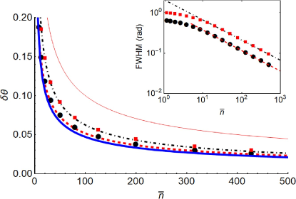
Figure 3: For given $\sinh^{2}r=0.687$ (i.e., $e^{-r}=0.47$) and the purity $\varrho=0.58$, the best sensitivity as a function of $\bar{n}$ for the multi-outcome measurement with $a=0.1$ (solid circles), and that of the binary-outcome measurement with $a=0.5$ (red squares) and $a\rightarrow\infty$ (blue thick line, given by Eq. (7)). Red thin line: the SNL. Dot-dashed line: $\delta\theta_{\mathrm{bin,\min}}\sim 0.75/\bar{n}^{0.54}$; Red dashed line: $\delta\theta_{\mathrm{mul,\min}}\sim 1.1e^{-r}/\sqrt{\bar{n}}$. Inset: the FWHM of the scaled $P_{0}(\theta)$ as a function of $\bar{n}$ for $a=0.5$ (red squares) and $0.1$ (solid circles). The dot-dashed line in the inset: $(2\pi/3)/\sqrt{\bar{n}}$; The red dashed line: $1.21/\bar{n}^{0.51}$.

To saturate the CRB, we adopt two estimation protocols based on the single-port homodyne detection in the squeezed-state interferometer. The first one is maximum-likelihood estimation. It is well known that the MLE is unbiased and can saturate the CRB when ${\mathcal{N}}\gg 1$ (see e.g. Ref. Helstrom ). Numerically, the estimator $\theta_{\mathrm{mle}}$ can be determined by maximizing the likelihood function (i.e., a multinomial distribution):

$$\mathcal{P}(\theta|\{{\mathcal{N}}_{k}\})={\mathcal{N}}!\prod_{k}\frac{1}{{\mathcal{N}}_{k}!}\left[P_{k}^{\mathrm{(fit)}}(\theta)\right]^{{\mathcal{N}}_{k}},$$ (18)

where ${\mathcal{N}}_{k}={\mathcal{N}}_{k}(\theta_{0})$ denotes the occurrence number of each outcome at a given true value of phase shift $\theta_{0}$, and $P_{k}^{\mathrm{(fit)}}(\theta)$ is a fit of the averaged occurrence frequency. To speed up numerical simulations, we directly use the analytical results of $P_{k}(\theta)$. For large enough $\mathcal{N}$, the phase distribution can be well approximated by a Gaussian Jin :

$$\mathcal{P}(\theta|\{{\mathcal{N}}_{k}\})\varpropto\exp\left[-\frac{(\theta-\theta_{\mathrm{mle}})^{2}}{2\sigma^{2}}\right],$$ (19)

where $\sigma$ is $68.3\%$ confidence interval of the Gaussian around $\theta_{\mathrm{mle}}$, determined by

$$\sigma\approx\sqrt{\frac{1}{\left|\partial^{2}\mathcal{P}(\theta|\{{\mathcal{N}}_{k}\})/\partial\theta^{2}\right|}}.$$ (20)

In Fig. 4(c), we plot the averaged phase uncertainty per measurement $\sqrt{{\mathcal{N}}}\sigma$ (see the circles) and its standard derivation (the bars) for each given $\theta_{0}$, using $M$ replicas of ${\mathcal{N}}$ random numbers. One can find that the circles follows the blue solid line (i.e., $\delta\theta_{\mathrm{mul}}$). Furthermore, from Fig. 4(d), one can find that standard derivation of $\theta_{\mathrm{mle}}$ (the bars) is larger than averaged value of the error $(\theta_{\mathrm{mle}}-\theta_{0})$, indicating that $\theta_{\mathrm{mle}}$ is unbiased Pezze .

A new phase-estimation protocol can be obtained from a convex combination of the CFI of each outcome $f_{k}(\theta)$. First, we define the inversion estimator of each outcome $\theta_{\mathrm{inv},k}=P_{k}^{-1}({\mathcal{N}}_{k}/{\mathcal{N}})$ by inverting the equation $P_{k}(\theta)={\mathcal{N}}_{k}/{\mathcal{N}}$. Next, we construct a composite phase estimator with the weight determined by $f_{k}(\theta)$,

$$\theta_{\mathrm{est}}=\sum_{k}c_{k}\theta_{\mathrm{inv},k},\text{ \ \ \ }c_{k}=\frac{f_{k}\left(\theta_{\mathrm{inv},k}\right)}{\sum_{k}f_{k}\left(\theta_{\mathrm{inv},k}\right)},$$ (21)

where $f_{k}(\theta)$ has been defined by Eq. (17), with $k=0$, $\pm$ for the multi-outcome homodyne measurement. Obviously, this result is physically intuitive. For example, if the CFI of the outcome $k=0$ dominates over that of the others (so that $\theta_{\mathrm{inv},0}$ is much more reliable than $\theta_{\mathrm{inv},\pm}$), then the above equation reduces to $\theta_{\mathrm{est}}\approx\theta_{\mathrm{inv},0}$. Furthermore, this estimator enjoys the good merits of the inversion estimator (i.e., the simplicity) and the well-known maximum-likelihood estimator (i.e., unbiasedness and asymptotic optimality in the sensitivity). In Fig. 4(e) and (f), we numerically obtain the estimators $\{\theta_{\mathrm{est}}^{(1)},\theta_{\mathrm{est}}^{(2)},\cdots,\theta_{\mathrm{est}}^{(M)}\}$ using $M$ replicas of ${\mathcal{N}}$ random numbers at each given $\theta_{0}$. Unlike the MLE, the performance of $\theta_{\mathrm{est}}$ is simply determined by the root-mean-square fluctuation

$$\sigma_{\mathrm{est}}=\sqrt{\langle(\theta_{\mathrm{est}}^{(i)}-\theta_{0})^{2}\rangle_{s}},$$ (22)

where $\langle(\cdots)\rangle_{s}\equiv\sum_{i=1}^{M}(\cdots)/M$ denotes the statistical average. As shown in Fig. 4(e) and (f), one can find that the averaged phase uncertainty per measurement $\sqrt{{\mathcal{N}}}\sigma_{\mathrm{est}}$ almost follows the CRB $\delta\theta_{\mathrm{mul}}$ and the bias $\langle\theta_{\mathrm{est}}\rangle_{s}-\theta_{0}$ is almost vanishing, similar to the MLE.

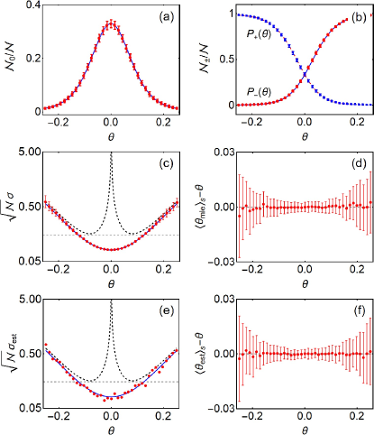
Figure 4: With $M=100$ replicas of ${\mathcal{N}}=1000$ random numbers at each given $\theta\in(-1/4,1/4)$, (a) and (b) statistical average of the occurrence frequencies ${\mathcal{N}}_{0}/{\mathcal{N}}$ and ${\mathcal{N}}_{\pm}/{\mathcal{N}}$ (solid circles) and their standard derivations (the bars), following $P_{0}(\theta)$ and $P_{\pm}(\theta)$. (c) and (e) The averaged phase uncertainty per measurement of $\theta_{\mathrm{mle}}$ and $\theta_{\mathrm{est}}$, following $\delta\theta_{\mathrm{mul}}$ (blue solid lines) and surpassing the phase sensitivity of the binary-outcome measurement $\delta\theta_{\mathrm{bin}}$ (dashed lines). (d) and (f) The bias of $\theta_{\mathrm{mle}}$ and $\theta_{\mathrm{est}}$ (solid circles), smaller than their standard derivations (the bars), indicating unbiasedness of them. The horizontal lines in (c) and (e): the $\mathrm{SNL}$. Other parameters: $\varrho=0.58$, $a=0.1$, $\alpha_{0}^{2}=42$, and $\sinh^{2}r=0.687$ ($e^{-r}=0.47$).

It should be mentioned that the dashed lines in Fig. 4(c) and (e) show the sensitivity of the binary-outcome scheme $\delta\theta_{\mathrm{bin}}$, which can beat the $\mathrm{SNL}$ if one takes $a=0.5$ (see Ref. Schafermeier ). Based on Eq. (15), one can also investigate the performance of the simplest inversion estimation $\theta_{\mathrm{inv}}$, which depends on the choice of the eigenvalues $\mu_{k}$ Wang . When $\mu_{+}=\mu_{-}$, it is simply given by $\delta\theta_{\mathrm{bin}}$. For other choices of $\{\mu_{k}\}$, the performance of $\theta_{\mathrm{inv}}$ cannot outperform that of the MLE and hence the new estimator $\theta_{\mathrm{est}}$, as predicted by the Crámer-Rao inequality Helstrom ; Braunstein1 ; Braunstein2 ; Paris2009 . Finally, in addition to the squeezed-state light interferometry, we believe that our estimation protocol may also be applicable to other kinds of multi-outcome measurements (e.g., intensity-difference measurement over the twin-Fock states TFs , which will be shown elsewhere).

V Conclusion

In summary, we have proposed a new data-processing method for the homodyne detection at one port of squeezed-state light interferometer, where the measurement quadrature are divided into three bins: $p\in(-\infty,-a)$, $[-a,a]$, and $(a,\infty)$, corresponding to a multi-outcome measurement. Compared with previous binary-outcome case Schafermeier , we show that (i) the divergence of phase sensitivity at $\theta=0$ can be removed, which is useful for estimating a small phase shift; (ii) Higher improvement in the resolution and the sensitivity is achievable with the realistic experimental parameters. For instance, we obtain a $38$-fold improvement in the resolution with the average number of photons $\bar{n}\sim 427$, while the sensitivity $\sim 1.1e^{-r}/\sqrt{\bar{n}}$, almost approaching the best sensitivity of the single-port homodyne measurement without any data-processing. Furthermore, a new phase-estimation protocol has been developed based on a combination of the inversion estimators of each outcome. Similar to the well-known maximum-likelihood estimator, we show that the estimator is unbiased and its uncertainty can saturate the Cramér-Rao bound of phase sensitivity. Our estimation protocol may also be applicable to other kinds of multi-outcome measurements.

Appendix A Details of Eq. (3)

The output state is given by $|\psi_{\mathrm{out}}(\theta)\rangle=\hat{U}(\theta)|\psi_{\mathrm{in}}\rangle$, where $\hat{U}(\theta)$ is an unitary operator

$$\hat{U}(\theta) = \exp\left(-i\frac{\pi}{2}\hat{J}_{y}\right)\exp\left(-i\theta\hat{a}^{{\dagger}}\hat{a}\right)\exp\left(-i\frac{\pi}{2}\hat{J}_{y}\right)$$ (23)

$$= \exp\left(-i\pi\hat{J}_{y}\right)\exp\left(i\theta\hat{G}\right),$$

which represents a sequence actions of the 50:50 beamsplitter at the output port Gerrybook , the phase accumulation at one of the two paths, and the 50:50 beamsplitter at the input port. For brevity, we have introduced Schwinger’s representation of the angular momentum $\hat{J}=\frac{1}{2}(\hat{a}^{{\dagger}},\hat{b}^{{\dagger}})\hat{\sigma}\binom{\hat{a}}{\hat{b}}$ and $\hat{G}=\hat{J}_{x}-\hat{n}/2$, with the Pauli matrix $\hat{\sigma}=(\hat{\sigma}_{x},\hat{\sigma}_{y},\hat{\sigma}_{z})$ and $\hat{n}=\hat{a}^{{\dagger}}\hat{a}+\hat{b}^{{\dagger}}\hat{b}$.

The ultimate phase-estimation precision is determined by the so-called quantum Cramér-Rao bound Helstrom ; Braunstein1 ; Braunstein2 ; Paris2009 : $\delta\theta_{\mathrm{QCRB}}=1/\sqrt{F_{Q}}$, where $F_{Q}$ is the quantum Fisher information. For the unitary operator $\hat{U}(\theta)$ and the squeezed-state input state $|\psi_{\mathrm{in}}\rangle=|\alpha_{0}\rangle\otimes|\xi_{0}\rangle$, it is simply given by

$$F_{Q}=4\left(\Delta\hat{G}\right)_{\mathrm{in}}^{2}=4\left[\left\langle\hat{J}_{x}^{2}\right\rangle_{\mathrm{in}}+\frac{\left(\Delta\hat{n}\right)_{\mathrm{in}}^{2}}{4}\right],$$ (24)

which is optimal when the phases of the two incident light fields satisfy the phase-matching condition $\cos(\arg\xi_{0}-2\arg\alpha_{0})=-1$, e.g., $\arg\alpha_{0}=0$ and $\arg\xi_{0}=\pi$ LPan1 ; LPan2 ; LJing .

For the homodyne detection at one of two ports of the interferometer, the conditional probability for detecting a measurement quadrature $p\in(-\infty,\infty)$ is given by

$$P(p_{a}|\theta)=\int_{-\infty}^{\infty}dx_{a}\int_{-\infty}^{\infty}dx_{b}\int_{-\infty}^{\infty}dp_{b}W_{\mathrm{out}}(\alpha,\beta;\theta),$$ (25)

where $\alpha=x_{a}+ip_{a}$ and $\beta=x_{b}+ip_{b}$. The Wigner function of the output state is given by Wang

$$W_{\mathrm{out}}(\alpha,\beta;\theta)=W_{\mathrm{in}}(\tilde{\alpha}_{\theta},\tilde{\beta}_{\theta}),$$ (26)

where

$$\left\{\begin{array}[]{l}\tilde{\alpha}_{\theta}=\alpha\frac{e^{i\theta}-1}{2}+\beta\frac{e^{i\theta}+1}{2},\\ \tilde{\beta}_{\theta}=-\alpha\frac{e^{i\theta}+1}{2}-\beta\frac{e^{i\theta}-1}{2}.\end{array}\right.$$ (27)

Note that Eqs. (25)-(27) hold for the two-path interferometer described by $\hat{U}(\theta)$, independent from specific form of the input state. For the input state $|\alpha_{0}\rangle\otimes|\xi_{0}\rangle$, we obtain the conditional probabilities for detecting a field quadrature at one port of the squeezing-state interferometer, as Eq. (3) in main text.

References

- (1) L. Pezzé, A. Smerzi, M. K. Oberthaler, R. Schmied, and P. Treutlein, “Quantum metrology with nonclassical states of atomic ensembles,” Rev. Mod. Phys. 90, 035005 (2018).
- (2) J. Ma, X. Wang, C. P. Sun, and F. Nori, “Quantum spin squeezing,” Phys. Rep. 509, 89 (2011).
- (3) J. P. Dowling, “Quantum optical metrology-the lowdown on high-N00N states,” Contemp. Phys. 49, 125-143 (2008).
- (4) A. N. Boto, P. Kok, D. S. Abrams, S. L. Braunstein, C. P. Williams, and J. P. Dowling, “Quantum Interferometric Optical Lithography: Exploiting Entanglement to Beat the Diffraction Limit,” Phys. Rev. Lett. 85, 2733 (2000).
- (5) V. Giovannetti, S. Lloyd, and L. Maccone, “Quantum-Enhanced Measurements: Beating the Standard Quantum Limit,” Science 306, 1330 (2004).
- (6) G. A. Durkin, and J. P. Dowling, “Local and Global Distinguishability in Quantum Interferometry,” Phys. Rev. Lett. 99, 070801 (2007).
- (7) C. C. Gerry, and R. A. Campos, “Generation of maximally entangled states of a Bose-Einstein condensate and Heisenberg-limited phase resolution,” Phys. Rev. A 68, 025602 (2003).
- (8) D. Braun, G. Adesso, F. Benatti, R. Floreanini, U. Marzolino, M. W. Mitchell, and S. Pirandola, “Quantum-enhanced measurements without entanglement,” Rev. Mod. Phys. 90, 035006 (2018).
- (9) U. Dorner, R. Demkowicz-Dobrzanski, B. J. Smith, J. S. Lundeen, W. Wasilewski, K. Banaszek, and I. A. Walmsley, “Optimal Quantum Phase Estimation,” Phys. Rev. Lett. 102, 040403 (2009).
- (10) Y. M. Zhang, X. W. Li, W. Yang, and G. R. Jin, “Quantum Fisher information of entangled coherent states in the presence of photon loss,” Phys. Rev. A 88, 043832 (2013).
- (11) K. J. Resch, K. L. Pregnell, R. Prevedel, A. Gilchrist, G. J. Pryde, J. L. O’Brien, and A. G. White, “Time-Reversal and Super-Resolving Phase Measurements,” Phys. Rev. Lett. 98, 223601 (2007).
- (12) Y. Gao, P. M. Anisimov, C. F. Wildfeuer, J. Luine, H. Lee, and J. P. Dowling, “Super-resolution at the shot-noise limit with coherent states and photon-number-resolving detectors,” J. Opt. Soc. Am. B 27, A170-A174 (2010).
- (13) L. Cohen, D. Istrati, L. Dovrat, and H. S. Eisenberg, “Super-resolved phase measurements at the shot noise limit by parity measurement,” Opt. Express 22, 11945-11953 (2014).
- (14) E. Distante, M. Ježek, and U. L. Andersen, “Deterministic Superresolution with Coherent States at the Shot Noise Limit,” Phys. Rev. Lett. 111, 033603 (2013).
- (15) C. Schafermeier, M. Jezex, L. S. Madsen, T. Gehring, and U. L. Andersen, “Deterministic phase measurements exhibiting super-sensitivity and super-resolution,” Optica 5, 60-64 (2018).
- (16) The LIGO Scientific Collaboration, “A gravitational wave observatory operating beyond the quantum shot-noise limit,” Nature Phys. 7, 962 (2011).
- (17) The LIGO Scientific Collaboration, “Enhanced sensitivity of the LIGO gravitational wave detector by using squeezed states of light,” Nature Photon. 7, 613 (2013).
- (18) S. T. Pradyumna, E. Losero, I. Ruo-Berchera, P. Traina, M. Zucco, C. S. Jacobsen, U. L. Andersen, I. P. Degiovanni, M Genovese, and T. Gehring, “Quantum-enhanced correlated interferometry for fundamental physics tests,” arXiv:1810.13386[quant-ph].
- (19) X. M. Feng, G. R. Jin, and W. Yang, “Quantum interferometry with binary-outcome measurements in the presence of phase diffusion,” Phys. Rev. A. 90, 013807 (2014).
- (20) L. Ghirardi, I. Siloi, P. Bordone, F. Troiani, and M. G. A. Paris, “Quantum metrology at level anticrossing,” Phys. Rev. A 97, 012120 (2018).
- (21) G. R. Jin, W. Yang, and C. P. Sun, “Quantum-enhanced microscopy with binary-outcome photon counting,” Phys. Rev. A 95, 013835 (2017).
- (22) B. Yurke, S. L. McCall, and J. R. Klauder, “SU(2) and SU(1,1) interferometers,” Phys. Rev. A 33, 4033 (1986).
- (23) L. Pezzé, A. Smerzi, G. Khoury, J. F. Hodelin, and D. Bouwmeester, “Phase Detection at the Quantum Limit with Multiphoton Mach-Zehnder Interferometry,” Phys. Rev. Lett. 99, 223602 (2007).
- (24) C. M. Caves, “Quantum-mechanical noise in an interferometer,” Phys. Rev. D 23, 1693 (1981).
- (25) L. Pezzé and A. Smerzi, “Mach-Zehnder Interferometry at the Heisenberg Limit with Coherent and Squeezed-Vacuum Light,” Phys. Rev. Lett. 100, 073601 (2008).
- (26) J. Liu, X. Jing, and X. Wang, “Phase-matching condition for enhancement of phase sensitivity in quantum metrology,” Phys. Rev. A 88, 042316 (2013).
- (27) P. Liu, P. Wang, W. Yang, G. R. Jin, and C. P. Sun, “Fisher information of a squeezed-state interferometer with a finite photon-number resolution,” Phys. Rev. A 95, 023824 (2017).
- (28) P. Liu, and G. R. Jin, “Ultimate phase estimation in a squeezed-state interferometer using photon counters with a finite number resolution,” J. Phys. A: Math. Theor. 50, 405303 (2017).
- (29) C. C. Gerry and P. L. Knight, Introductory Quantum Optics (Cambridge University, 2005).
- (30) K. P. Seshadreesan, P. M. Anisimov, H. Lee, and J. P. Dowling, “Parity detection achieves the Heisenberg limit in interferometry with coherent mixed with squeezed vacuum light,” New J. Phys. 13, 083026 (2011).
- (31) Q. S. Tan, J. Q. Liao, X. G. Wang, and F. Nori, “Enhanced interferometry using squeezed thermal states and even or odd states,” Phys. Rev. A 89, 053822 (2014).
- (32) J. Z. Wang, Z. Q. Yang, A. X. Chen, W. Yang, and G. R. Jin, “Multi-outcome homodyne detection in a coherent-state light interferometer,” Opt. Express 27, 10343 (2019).
- (33) C. W. Helstrom, Quantum Detection and Estimation Theory (Academic, New York, 1976).
- (34) S. L. Braunstein, and C. M. Caves, “Statistical distance and the geometry of quantum states,” Phys. Rev. Lett. 72, 3439 (1994).
- (35) S. L. Braunstein, C. M. Caves, and G. J. Milburn, “Generalized uncertainty relations: Theory, examples, and Lorentz invariance,” Ann. Phys. (NY) 247, 135 (1996).
- (36) M. G. A. Paris, “Quantum estimation for quantum technology,” In. J. Quantum Inform. 7, 125 (2009).
- (37) M. J. Holland and K. Burnett, “Interferometric detection of optical phase shifts at the Heisenberg limit” Phys. Rev. Lett. 71, 1355 (1993).