Type IIP Supernova Progenitors II: Stellar Mass and Obscuration by the Dust in the Circumstellar Medium

Abstract

It has been well established from a variety of observations that red supergiants (RSGs) loose a lot of mass in stellar wind. emitted gas over a few decades before core-collapse can lead to substantial extinction and obscure the intrinsic luminosity of the progenitor RSG. This may lead to a difficulty in determining the range of progenitor masses that lead to the different classes of supernovae. Even the , well studied supernovae with pre-explosion observations, such as SN 2013ej may suffer from this uncertainty in the progenitor mass. We explore masses proposed for its progenitor using Modules for Experiments in Stellar Astrophysics (MESA). We show that a non-rotating star with the initial mass of 26 M_⊙ would require a considerable amount of circumstellar medium to obscure its high luminosity the observed pre-explosion magnitudes detected by the Hubble Space Telescope (HST). Such a high value of visual extinction appears to be inconsistent with that derived for SN 2013ej as well as SN 2003gd in the same host galaxy M74. In contrast, the evolutionary models of lower mass (13 M_⊙) star are easily accommodated within the observed HST magnitudes. Some of the 26 M_⊙ simulations show luminosity variation in the last few years which could be discriminated by high cadence and multiband monitoring of supernova candidates in nearby galaxies. We demonstrate that our calculations are well resolved with adequate zoning and evolutionary time-steps.

1 Introduction

Core-collapse Supenovae (CCSNe) occur as a result of gravitational collapse of massive stars (typically, $>$ 8 $\rm M_{\sun}$ at Zero Age Main Sequence, ZAMS) at the end of their evolution. A volume limited sample of CCSNe within 60 Mpc (Smith et al., 2011) shows that nearly 48% of these are supernovae of Type IIP, which have progenitors with a large hydrogen rich envelope at the time of their explosion. Because of the observational constraints, the progenitors corresponding to supernovae can be identified only for relativity nearby cases (at $d\leq 30\rm\;Mpc$). SN 2013ej (catalog ), a type IIP SN like its predecessor SN 2003gd (catalog ), occurred in the same host galaxy M74 at a distance of 9.0${}^{+0.4}_{-0.6}$ Mpc (Dhungana et al., 2016) and was followed extensively by many groups in UV, optical, infrared bands (Yuan et al., 2016; Huang et al., 2015; Bose et al., 2015; Richmond, 2014; Fraser et al., 2014; Valenti et al., 2014) and in X-ray bands (Chakraborti et al., 2016). The estimated mass of the progenitor of SN 2013ej in the literature ranges between 11–16 $\rm M_{\sun}$, while the X-ray measurement of Chakraborti et al. (2016) points to a ZAMS mass of 13.7 $\rm M_{\sun}$ for the progenitor. Das & Ray (2017) restrict the ZAMS mass of the progenitor star of SN 2013ej using the archival HST observations and their simulations to an upper bound of 14 $\rm M_{\sun}$. They also show through their 1-D simulations of evolution of a 13 $\rm M_{\sun}$ star and its explosion that the observed light curves are fitted well with their simulations, when they included enhanced mass loss towards the end stages of evolution of the star. On the other hand, Utrobin & Chugai (2017) argue for a significantly higher progenitor mass of 25.5–29.5 $\rm M_{\sun}$ on the main sequence (and the ejecta mass of 23–26 $\rm M_{\sun}$) based on arguments of high velocity $\rm Ni^{56}$ ejecta. They also claim that a sufficient mass loss rate can produce a circum-stellar envelope at a distance about $\rm 10^{15}$ cm that would hide the pre-SN light from such a massive progenitor star.

We present here a few cases of an isolated (single), non-rotating and non-magnetized star as a progenitor of SN 2013ej for two fixed ZAMS masses of 13 $\rm M_{\sun}$ and 26 $\rm M_{\sun}$. In the companion Paper I (Wagle et al., 2019), we have studied in detail the effect of convective overshoot on the evolution and explodibility of the progenitor for ZAMS mass of 13 $\rm M_{\sun}$. test the case of a 26 $\rm M_{\sun}$ star as a possible progenitor of SN 2013ej. We study its luminosity variations in the late stages of stellar evolution and calculate its visual extinction due to dust formation in the circumstellar medium (CSM) formed by mass loss through stellar wind and compare these with archival observations of the progenitor star. We also demonstrate that our models have adequately fine mass resolution In our future work, we will simulate the explosion of these models through 1-D SN explosion codes and compare with the observed light curves and expansion velocity profiles to test the viability of the models.

In section 2, we describe the methods of computational simulations and the stellar evolution using MESA. In section 3, we discuss the results of variation of different MESA parameters on the stellar structure for our models. We also show that our models have adequate mass resolution. We discuss the extinction due to dust (formed in the CSM) on the observed magnitudes of the progenitor star. In section 4, we discuss and summarize our conclusions.

Table 1: Inlist parameters & MESA predicted core properties for $\rm M_{ZAMS}$ = 13 $\rm M_{\sun}$ & 26 $\rm M_{\sun}$ models with Z = 0.006 and $f$ = 0.025

dm	overshoot	delta$\_$lg$\_$X$\_$cntr$\_$limit/hardlimit			Max dt	Dutch Wind	Network	model id	$\rm He_{core}$	$\rm C_{core}$	$\rm O_{core}$	$\rm Si_{core}$	$\rm Fe_{core}$
($\rm M_{\odot}$)	parameter, $f_{0}$	Ne	O	Si	Change	$\eta$	size
MZAMS = 13 $\rm M_{\odot}$									MZAMS = 13 $\rm M_{\odot}$
0.007	0.050	0.02/0.03	0.02/0.03	0.02/0.03	1.15	0.5	22 isotopes	13$\rm M_{\odot}$  model 10		2.108	2.056	1.576	1.477	0.029
0.007	0.005	0.02/0.03	0.02/0.03	0.02/0.03	1.15	0.5	22 isotopes	13$\rm M_{\odot}$  model 20		2.179	2.120	1.611	1.510	0.035
0.007	0.005	0.02/0.03	0.02/0.03	0.02/0.03	1.15	0.5	79 isotopes	13$\rm M_{\odot}$  model 30		2.187	1.898	1.545	1.481	0.030
0.01	0.050	0.02/0.03	0.02/0.03	0.02/0.03	1.15	1.0	22 isotopes	13$\rm M_{\odot}$   model 40		2.102	2.052	1.591	1.495	–
0.007	0.050	0.02/0.03	0.02/0.03	0.02/0.03	1.2/1.15	0.5	45/204 isotopes	13$\rm M_{\odot}$  model 5		2.059	1.929	1.497	1.365	–
–	0.005	–	–	–	1.20	0.5	21 isotopes	13$\rm M_{\odot}$   modified test suite		2.147	1.969	1.593	1.468	0.034
MZAMS = 26 $\rm M_{\odot}$									MZAMS = 26 $\rm M_{\odot}$
0.007	0.050	0.02/0.03	0.02/0.03	0.02/0.03	1.20	0.5	22 isotopes	26$\rm M_{\odot}$  model 10		4.610	1.889	0.000	1.529	0.128
0.01	0.050	0.015/0.03	0.015/0.03	0.015/0.03	1.20	0.5	22 isotopes	26$\rm M_{\odot}$  model 2		3.262	2.948	1.729	1.589	0.187
0.01	0.020	0.01/0.02	0.01/0.02	0.01/0.02	1.20	0.5	22 isotopes	26$\rm M_{\odot}$  model 30		3.952	3.820	1.690	1.538	0.151
0.01	0.050	0.01/0.02	0.02/0.04	0.01/0.02	1.20	0.5	79 isotopes	26$\rm M_{\odot}$  model 4		3.253	2.963	1.811	1.587	–
–	0.050	–	–	–	1.20	0.5	21 isotopes	26$\rm M_{\odot}$  modified test suite		5.294	2.427	1.660	1.508	0.138

Note. — delta$\_$lg$\_$X$\_$cntr$\_$limit & hardlimit values were set to 0.01 & 0.02, respectively through CC for H, He and C in all of the above models. See section 2 for more details on the choices of other parameters listed here.

2 Methods of Simulations

We use version r-10398 to explore the evolution of the presumed progenitor of SN 2013ej from the ZAMS stage through to the core-collapse (CC) stage. All the MESA inlists will be made available publicly at MESA market place (subject to acceptance of the manuscript). In the following subsections, we discuss the choices of a few important parameters that affect the results discussed in this paper.

2.1 Initial Mass and Abundances

As discussed in the introduction, we investigate isolated (single) star for two different cases of ZAMS masses of 13 $\rm M_{\sun}$ & 26 $\rm M_{\sun}$. The initial metallicity Z = 0.006 is used in our simulations to create a pre-MS model. When provided the Z value, MESA sets up the initial helium abundance (Y) to a value equal to 0.24 + 2$\rm\times Z_{initial}$ (refer to equations (1) through (3) of Choi et al., 2016). As a result, for our simulations the initial H abundance (X) was set up to 0.742 with Y = 0.252, since X+Y+Z = 1. MESA uses (Grevesse & Sauval, 1998) abundance values to derive the initial abundances for each of the metals based on the choice of initial Z. The Grevesse & Sauval (1998) solar values for helium and metal abundances are $\rm Y_{\sun}$ = 0.2485 and $\rm Z_{\sun}$ = 0.0169, respectively.

2.2 Mass and Temporal Resolution

In our simulations, we the mass and temporal resolution controls Farmer et al. (2016).

The time-step between consecutive models in a simulation is generally controlled by varcontrol$\_$target. . We set it to its MESA default value of $\rm 10^{-4}$.

This set of limits ensure the convergence of mass shell locations, smoother transition in the HRD at the “Henyey Hook” (Kippenhahn et al., 2012), and smoother trajectories in the central temperature-density ($\rm T_{c}-\rho_{c}$) plane. For a few of our model simulations we had to relax some of these limits at steps where we encountered convergence problems (refer to Table 1 for details).

2.3 Opacities and Equation of State

We have used Type II opacity tables (Iglesias & Rogers, 1996) that take into account varying C & O abundances beyond that accounted for by Z. MESA uses Type I tables (Cassisi et al., 2007) instead of Type II tables where metallicity is not significantly higher than Zbase. We set Zbase to the same value as initial Z = 0.006. MESA uses HELM EOS to account for an important opacity enhancement during pair production because of increasing number of electrons and positrons per baryon, at late stages of nuclear burning.

MESA uses equation of states tables based on OPAL tables (Rogers & Nayfonov, 2002), and at lower densities and temperatures SCVH tables (Saumon et al., 1995) with a smooth transition between these tables in the overlapping region defined by MESA.

2.4 Nuclear Reaction Rates and Networks

MESA mainly uses NACRE (Angulo et al., 1999) rates for thermonuclear reactions with updated triple-$\alpha$ (Fynbo et al., 2005) and $\rm{}^{12}C$($\alpha$,$\gamma$)$\rm{}^{16}O$ rates (Kunz et al., 2002) among others. (For more details see, Paxton et al., 2011, section 4.4).

In our model simulations

2.5 Mixing, Diffusion, and Overshoot

MESA uses standard mixing length theory (MLT) of convection (Cox & Giuli, 1968, chap.14). We used the Ledoux criterion in our simulations, instead of the Schwarzchild criterion to determine the convective boundaries (Paxton et al., 2013). We used $\rm\alpha_{MLT}=$ 2 Here the mixing length equals $\rm\alpha_{MLT}$ times the local pressure scale height, $\rm\lambda_{P}=P/g\rho$. We also enabled two time-dependent diffusive mixing processes, semiconvection and convective overshooting, in our simulations. Semiconvection refers to mixing in regions unstable to Schwarzchild criterion but stable to Ledoux, $\rm\nabla_{ad}<\nabla_{T}<\nabla_{L}$. Semiconvection only applies when Ledoux criterion is used in MESA. We set the dimensionless efficiency parameter, $\alpha_{SC}=$ 0.1 for efficient mixing . MESA’s treatment for overshoot mixing is described in our Paper I . For the simulations presented in this paper, we keep the $f$ value fixed at 0.025

Figure 1: The HRD comparing the evolution for different M_ZAMS = 13 $\rm M_{\sun}$ (a) & 26 $\rm M_{\sun}$ (b) simulations with initial Z=0.006 presented in this paper (see Table 1). The inset in panel (a) shows the whole evolution from ZAMS to CC. The 26 $\rm M_{\sun}$ models with lower mass resolution (dm = 0.01 $\rm M_{\sun}$) exhibit spirals (inset in panel (b)) in post Ne-ignition evolutionary track. These spirals go away with a higher mass resolution (dm = 0.007 $\rm M_{\sun}$, 26 $\rm M_{\sun}$ model 1), but it is unaffected by a finer temporal resolution (max change in dt = 1.15, model not shown here).

2.6 Mass Loss by Stellar Winds

For the “hot” phase, we used the “Vink” scheme (Vink et al., 2001) with $\eta_{Vink}$ = 1.0 (Vink$\_$scaling$\_$ factor) and for the “cool” phase, we used the “Dutch” wind scheme for both the AGB and the RGB phases, with $\eta_{Dutch}$ = 0.5 (Dutch$\_$scaling$\_$factor) in the simulations presented here. The particular combination used in MESA is based on Glebbeek et al. (2009). The MESA mass loss rates are switched between the rates of Vink et al. (2001, 2000) to that of de Jager et al. (1988) at temperatures below 10,000 K.

2.7 Stopping criterion

The model is stopped very close to the collapse of the star when the infall velocity at any location in the interior of the star reaches the fe$\_$core$\_$infall$\_$limit = $\rm 10^{8}$ $\rm cm~{}s^{-1}$. We turned on the velocity variable ‘v’ defined at cell boundaries, by setting v$\_$flag = .true. when the central electron fraction $\rm Y_{e}$ (electrons per baryon, $\rm\bar{Z}/\bar{A}$) drops below 0.47 (center$\_$ye$\_$limit$\_$for$\_$v$\_$flag). This enables MESA to compute hydrodynamic radial velocity, which is used for evaluating the stopping criterion.

Figure 2: The density (grey) and temperature (red) scale heights along with the mass resolutions (zoning, blue dotted line) for the M_ZAMS= 13 $\rm M_{\sun}$ model (a) & 26 $\rm M_{\sun}$ models (b,c) with Z = 0.006 at CC. The scale height M_x = (d ln x/dm)^-1 (Sukhbold et al., 2018) for a quantity ‘x’ to mass resolution ratio is an indicator of zoning efficiency. Panel (a) shows the 13 $\rm M_{\sun}$ model with dm = 0.007 $\rm M_{\sun}$, and panels (b) & (c) show 26 $\rm M_{\sun}$ models 1 & 2 with dm = 0.007 $\rm M_{\sun}$ and 0.01 $\rm M_{\sun}$, respectively. The fluctuations in density and the pressure scale heights is over-resolved in our simulations, which is apparent by the 2 dex fine zoning at most places.

3 Results

Table 2: Magnitudes and Dust Extinction for $\rm M_{ZAMS}$ = 26 $\rm M_{\sun}$, Z = 0.006 model 1

HST	Johnson	Synthetic	MESA	Min.	Calculated $A(\nu)$ for Graphite					Calculated
Observed	Band	Observed	Calculated	$A(\nu)$	minimum	Heat Balance		Adiabatic Cooling		$A(\nu)$ for
Magnitude		Magnitude	Magnitude	required	grain	$\rm T_{d,max}$	$\rm T_{d,max}$	$\rm T_{d,max}$	$\rm T_{d,max}$	Silicates
		($\rm m_{obs}$)	($\rm M_{MESA}+\mu_{d}$)		Å	1500	2000	1500	2000
$(\rm\tau_{CC}-\tau)\approx$ 10 yrs, $\rm R_{star}=1017.73~{}R_{\odot}$
25.16$\pm$0.09	V	24.99$\pm$0.13	21.91	3.08	800	1.35	3.89	4.51	5.28	0.74
					1500	1.13	3.27	3.80	4.44
22.66$\pm$0.03	I	22.70$\pm$0.09	20.40	2.30	800	0.65	1.86	2.16	2.53	0.36
					1500	0.54	1.57	1.82	2.13
$(\rm\tau_{CC}-\tau)\approx$ 8 yrs, $\rm R_{star}=1017.69~{}R_{\odot}$
24.84$\pm$0.05	V	24.69$\pm$0.08	21.91	2.78	800	1.35	3.90	4.51	5.32	0.74
					1500	1.14	3.28	3.79	4.47
22.66$\pm$0.03	I	22.69$\pm$0.08	20.40	2.29	800	0.65	1.87	2.16	2.55	0.36
					1500	0.54	1.57	1.82	2.14

Note. — The calculated (absolute) magnitudes from our MESA simulation are listed along with the observed HST WFC magnitudes in F555W & F814W bands from Fraser et al. (2014). The dust extinction values calculated using the formalism explained in Appendix A are listed here.

3.1 HR diagram & mass resolution

On the other hand, we notice that the effects of choices of parameters are more prominent in the 26 $\rm M_{\sun}$ model, especially with dm which controls the minimum level of mass resolution. The most variation in luminosity takes place in model 2 (red) between 1.3 years and 0.6 years before collapse from log L = 5.4 to 5.5 (see the inset in panel (b)). , which can be easily observed. Unfortunately, observations only about 8 & 10 years before its collapse. The variation in magnitudes the spirals are not exhibited in model 1 that uses a dm The modified test suite models for both the ZAMS masses explored here are presented for comparison purpose only. The test suite models suffer from lack of strict temporal and mass resolution, the effect of which is prominent in the inset of panel (b) for 26 $\rm M_{\sun}$.

Sukhbold et al. (2018) for adequate zoning is that the key variables like density and temperature do not vary significantly between consecutive zones. In Fig. 2, we plot density and pressure scale heights along with the mass resolution 13 $\rm M_{\sun}$ model 3 with dm = 0.007 is shown in panel (a) and the 26 $\rm M_{\sun}$ models 2 & 3 with dm = 0.007 $\rm M_{\sun}$ and 0.01 $\rm M_{\sun}$ are shown in panels (b) & (c), respectively. A scale height for a quantity ’x’ is defined as M_x = (d ln x/dm)^-1, where an absolute value of M_x is considered. The large upward spikes in Fig. 2 represent regions of near constant temperature and density. The discontinuities in mean molecular weight at the edge of convective shells result in quantities being artificially small. The edge of the helium convective shell (mass coordinate $\sim$ 4 $\rm M_{\sun}$ in 13 $\rm M_{\sun}$ model and 8 $\rm M_{\sun}$ in 26 $\rm M_{\sun}$ model) shows steep gradient where the density changes by a few orders of magnitude, where the zoning is not well resolved. A finer resolution comes at a cost of increased computational time. Other than the edge of He shell, the zoning is 2 dex finer than the scale heights indicating that the quantities are over-resolved .

3.2 Dust Extinction for 26 $\rm M_{\sun}$ progenitor

Table 1 of Fraser et al. (2014) lists the observed magnitudes from archival pre-explosion images of the progenitor for SN 2013ej. The observations made in Nov 2003 & June 2005 are available, at about 10 and 8 years before the collapse of the star. We converted the HST observed magnitudes in F555 and F814 bands to Johnson’s photometric magnitudes V and I using formalism explained by Sirianni et al. (2005). To compare the MESA calculated V & I magnitudes to the observations, we evaluated the dust extinction due to the stellar wind formed by circum-stellar medium (CSM), using the formalism provided in Appendix A. These values are listed in Table 2 along with the HST observed magnitudes and the MESA calculated magnitudes for . We notice that the V band magnitude is reduced by about 0.3 mag in $\sim$2 years from 2003 to 2005. Our calculations do not show such variations for any of our 13 $\rm M_{\sun}$ or 26 $\rm M_{\sun}$ simulations between 10 to 8 years before collapse.

We see from Table 2 that a minimum A${}_{\rm V}\approx$ 2.8 – 3.1 is required to shield our fiducial 26 $\rm M_{\sun}$ progenitor. Although we see such high numbers among our calculated A_V values (columns (6) through (10) in the table), is significantly higher compared with the value of 0.45${}^{+0.04}_{-0.04}$ calculated by Maund (2017) in the host for the progenitor of SN 2013ej through Bayesian analysis of stellar population, using archival pre-SN data. As the host galaxy M74 is observed face-on, most of this extinction would be due to the CSM around the star. For another supernova of Type IIP, SN 2003gd in the same host galaxy M74 as SN 2013ej, Maund (2017) calculates A_V = 0.46${}^{+0.04}_{-0.03}$.

3.3 Central Temperature versus Density

Fig. 3 shows evolution of central temperature and density from ZAMS through CC. The 13 $\rm M_{\sun}$ models shown in panel (a) are in a good agreement until about when C-burning starts ($log_{10}T_{c}\approx$ 8.9 and $log_{10}\rho_{c}\approx$ 5.5). The 26 $\rm M_{\sun}$ models shown in panel (b) diverge after TAMS stage ($log_{10}T_{c}\approx$ 8 and $log_{10}\rho_{c}\approx$ 2). We notice that models with smaller network size tend to be hotter and less dense at the center through various burning stages. The insets in both the panels show evolutionary tracks during core O-burning and core Si-burning stages. We note that the tracks in this part , more so during core Si-burning, indicating that these phases of nuclear burning are challenging due to very high and nearly balancing reaction rates, as also pointed out in Renzo et al. (2017).

Figure 3: $\rho_{c}-$ T_c plot comparing the M_ZAMS= 13 $\rm M_{\sun}$  and 26 $\rm M_{\sun}$ models, with Z = 0.006 described in Table 1. Panels (a) and (b) show the evolution from ZAMS through CC for 13 $\rm M_{\sun}$ and 26 Sun models respectively, while the two sets of insets in these show the same during O-ignition through Si burning. One can observe that there are wiggles present during O and Si burning stages in the plot, which in this case, are present in almost all of the models. The wiggles during O burning stage disappear in 26 $\rm M_{\sun}$ model when higher mass resolution (dm = 0.007 $\rm M_{\sun}$) is chosen. The wiggles may therefore be numerical artefacts.

3.4 The Kippenhahn diagram

The Kippenhahn diagram is an useful representation of the succession of various convective burning zones inside the star throughout its evolution. Fig. 4 26 $\rm M_{\sun}$ model 1 with dm = 0.007 $\rm M_{\sun}$ and $f_{0}$ = 0.050, model 3 with dm = 0.01 $\rm M_{\sun}$ and $f_{0}$ = 0.020, and model 4 with dm = 0.01 $\rm M_{\sun}$ and $f_{0}$ = 0.050. Model 1 & 3 both use 22 isotopes network while model 4 uses 79 isotopes network. Note that 26 $\rm M_{\sun}$ models 3 & 4 both exhibiting spirals in the HRD, have a distinct intermediate convective zone (ICZ) at the bottom of the convective hydrogen shell (at about 16 $\rm M_{\sun}$) starting at about a few thousand years before the collapse, albeit the ICZ being very limited in mass extent is missing in model 1 . The mass resolution affect the internal structure of the star. The various core boundaries in the (dm = 0.01 $\rm M_{\sun}$) models 1 & 4 are systematically lower than those in the (dm = 0.007 $\rm M_{\sun}$) model 1.

Figure 4: Kippenhahn (KH) diagram for the M_ZAMS= 26 $\rm M_{\sun}$ and Z = 0.006 models described in Table 1. Panel (a) shows model 1 with dm = 0.007 $\rm M_{\sun}$ and $f_{0}$ = 0.050, while panel (b) shows model 3 with dm = 0.01 $\rm M_{\sun}$ and $f_{0}$ = 0.020, both using 22 isotopes network. Panel (c) shows model 4 with dm = 0.01 $\rm M_{\sun}$ and $f_{0}$ = 0.050, with 79 isotopes network. Various core boundaries reported by MESA are marked in the diagram. By default, the core boundaries are determined by the point at which the mass fraction of the previous isotope decreases below a threshold value of 0.01 and where the same for the current isotope is above 0.1.

3.5 Entropy from Oxygen Burning Onward

Figure 5: Entropy profile evolution for the M_ZAMS= 13 $\rm M_{\sun}$ model 3 and 26 $\rm M_{\sun}$model 1, with Z = 0.006, described in Table 1. The total entropy per baryon, S/N_Ak is plotted as a function of mass co-ordinate in panel (a) for evolution from ZAMS through C-ignition and panel (b) from C-ignition through CC stages. The pre-SN entropy profile structure is a consequence of increased entropy due to losses due to neutrinos in late burning stages.

The entropy profiles at various stages are shown in Fig 5 show sharp increases at the boundaries of various fossil shell-burning zones. Due to high core temperatures, the core is cooled predominantly by neutrinos emitted by thermal processes rather than by radiation from carbon burning stage onwards. However, oxygen burning onwards, the non-thermal emission of neutrinos as a result of electron capture on nuclei and beta decay of others start contributing. These sharp entropy gradients that prevent the mixing and penetration of burning products lead to the onion-skin structure in the core with distinct elements (e.g. C, Ne, O, Si) . Panel (a) shows that as the star’s entropy in the core decreases, the entropy in the envelope increases with time, even though during the various nuclear burning stages the entropy profile remains flat for a large part of the star except near the surface of the star.

3.6 Mass loss rate as the star evolves

As discussed in the Methods section, we use a combination of mass loss rates calculated for hot stars as in Vink et al. (2001) appropriate for OB stars near the main sequence and The rates for red supergiants have been tested recently by Mauron & Josselin (2011) who found it consistent with the de Jager et al. (1988) rates. van Loon et al. (2005) however have considered RSGs believed to be dust-enshrouded and have argued for a much higher mass loss rate. Meynet et al. (2015) pointed out that these mass loss rates at a given luminosity can differ by more than two orders of magnitude.

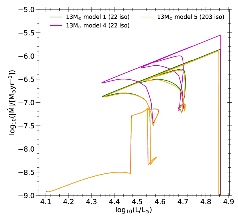
Figure 6: The figure shows mass loss rate as a function of luminosity (left) and $\rm T_{eff}$ (right) from ZAMS for various M_ZAMS= 13 $\rm M_{\sun}$ , Z = 0.006 models described in Tables 1.

In Fig. 6 we show the mass loss rate as a function of Luminosity for our fiducial 13 $\rm M_{\sun}$ . has a low mass loss rate of $\rm 10^{-9}$ $\rm M_{\sun}$ yr^-1 which climbs to a factor of roughly three times higher value as hydrogen in its core is depleted and its color evolves towards the red. At a luminosity about $\rm 3\times 10^{4}$ $\rm L_{\sun}$ (log L = 4.47) and a surface temperature of $\rm T_{eff}$ = 25,000 K, the mass loss rate undergoes a sharp increase by a factor of nearly 18, due to the so-called ”bi-stability jump” (Vink et al., 2001). The 26 $\rm M_{\sun}$ star also goes through the ”bi-stability jumps” after the TAMS loop and about $\rm 10^{6}$ yr before CC, but because it stays as a RSG, its mass loss evolution is somewhat simpler compared to that of a 13 $\rm M_{\sun}$ star. The 13 $\rm M_{\sun}$ star crosses this temperature several times near the terminal age main sequence (TAMS) stage. As a result the mass loss rate undergoes both sudden upward as well as downward transitions within a short range of luminosities.

In massive stars surface temperatures below 5000 K, dust begins to form in the stellar wind as the gas cools from the star. As the wind mass loss is driven by stellar luminosity, and the mass loss rate is one of the factors that determines the amount of dust formed, the dust production rate was found to correlate with the bolometric magnitude (Massey et al., 2005) as:

$$log\;\dot{M}_{dust}=-0.43M_{bol}-12.0$$

for stars with $M_{bol}<-5$ that corresponds to stars more massive than $>10\;M_{\odot}$. This gives a direct handle on how much dust formation is expected from a RSG of given luminosity at the end stage. The dust affects both stellar luminosity as well as color and its effects must be taken into account when comparing with observational color magnitude data. Dust formation and extinction due to dust are calculated in Appendix A and the results for a 26 $\rm M_{\sun}$ star and the corresponding V and I band calculated magnitudes are reported in Table 2 .

4 Summary and Discussion

Utrobin & Chugai (2017) claim that a progenitor star with a ZAMS mass of 27.5 $\pm$ 2 $\rm M_{\sun}$ with an ejecta mass of 23.1 – 26.1 $\rm M_{\sun}$ radius of 1500 $\rm R_{\sun}$ at pre-SN stage explains better the initial peak of the light curve. In addition, they argue that the bipolar ⁵⁶Ni distribution gives a better fit to the observed photospheric velocity profiles in their models. They prefer the 26 $\rm M_{\sun}$ ejecta model over the 23 $\rm M_{\sun}$ ejecta model. However, they do not give any explicit details about their pre-SN models, especially about the various physical parameters that would lead to such a progenitor star. We have run several MESA simulations to show that a star with ZAMS mass of 26 $\rm M_{\sun}$ will end up with a much smaller pre-SN mass of 22 – 23.5 $\rm M_{\sun}$ (including the collapsing core mass), even with a moderate mass loss rate ($\eta_{\rm Dutch}$ = 0.5) with the reasonable choices for other parameters for the evolution of the star. Our 26 $\rm M_{\sun}$ progenitor has a pre-SN radius of $\sim$1000 $\rm R_{\sun}$, while our 13 $\rm M_{\sun}$progenitor has a pre-SN radius of $\sim$660 $\rm R_{\sun}$. We also find that a higher ZAMS mass star with the same mass loss scheme produces even smaller pre-SN progenitor (see also fig. 3 of Ugliano et al., 2012, which shows a similar trend). In addition, a larger ZAMS mass (typically above 30 $\rm M_{\sun}$) would enter the Wolf-Rayet regime, reducing its chances to explode as a type II supernova.

As seen in Fig 1, such a massive star would be highly luminous (L_star/$\rm L_{\sun}$ $\sim$ a few times $\rm 10^{5}$) for most of its life before SN explosion. Such a star would require considerable amount of dust in the CSM to obscure the high luminosity. Even so, an observation in K band would not be affected by dust extinction. Unfortunately, we do not have any pre-explosion K band observations for the progenitor of SN 2013ej. As discussed in the Results section, our 26 $\rm M_{\sun}$ model 2 shows a large variation in luminosity in the final year before collapse, which results in both V & I band variation of 0.3 mag. This variation would not be affected by dust . such observations are not available for the progenitor of SN 2013 ej. Nevertheless, there exist HST observations for the progenitor star taken at about 8 & 10 years before the explosion. We calculate the extinction values using the CSM profiles calculated from the output of our MESA simulation for our fiducial ZAMS 26 $\rm M_{\sun}$ model 1 as discussed in Appendix A. These values are tabulated in Table 2. To dim a star as bright as a 26 $\rm M_{\sun}$ star, the amount of extinction required A_V would be of the order of 3 mag. Even value of A_V is 0.45 $\pm$ 0.04 determined by Maund (2017) in the host for SN 2013ej using archival pre-explosion observations through Bayesian analysis of stellar population. They also determined a value of A_V = 0.46${}^{+0.04}_{-0.03}$ for another type IIP SN 2003gd, which occurred in the same host galaxy. As this galaxy is observed face-on, most of this extinction would be due to the dust formed in the CSM around the progenitor star. This a ZAMS mass of 26 $\rm M_{\sun}$ for the progenitor star of SN 2013ej,

the progenitor of SN 2013ej than a star of about twice its mass detailed simulations of post-explosion multi-waveband light curves and Fe line velocity evolution to compare with available observational data .

Appendix A Extinction by Circum-Stellar Material

Here, we discuss our calculations for the extinction by dust particles (and the underlying assumptions) in the CSM formed by the mass lost in stellar winds (values listed in Table 2). The dust particles can form only when the wind moves sufficiently far from the star to avoid dust particles being eradicated by radiation near the star, and cools down to a temperature below dust destruction temperature. The typical value used in the literature for the sublimation temperature at which the dust particles will be destructed is $T_{d,max}$ = 1500 K (Das & Ray, 2017; Kochanek et al., 2012); however, the graphite dust particles can withstand temperatures as high as 2000 K (see, e.g., Fox et al., 2010). We calculate the minimum distance ($R_{min}$) from the stellar surface at which the dust can form, where the temperature of CSM falls below $\rm T_{d,max}$. Das & Ray (2017) determined this distance by simple adiabatic cooling of the wind ($\rm TV^{\gamma-1}=constant$) due to expansion with an adiabatic monotonic gas ($\gamma=\frac{5}{3}$). In this case, the minimum distance the gas has to travel to cool down below the graphite destruction temperature, considering dust temperature is same as that of the surrounding gas, is given as

$$R_{min}=R_{star}\sqrt{\frac{T_{star}}{T_{d,max}}}$$ (A1)

We use a more robust way of calculating the minimum distance using heat balance equation for dust grains in thermal equilibrium, where the rate of dust heating due to stellar radiation is equal to the rate of dust cooling due to thermal emission, written as (see, e.g. Draine & Lee, 1984; Kruegel, 2003)

$$\int_{0}^{\infty}Q_{abs}(a,\nu)\;J_{\nu,\;star}\;d\nu=\int_{0}^{\infty}Q_{abs}(a,\nu)\;B_{\nu}(T_{d})\;d\nu$$ (A2)

The absorption efficiency $Q_{abs}$ in mid-infrared where the grain emission takes place can be approximated to a power-law using a simple spherical grain model (Kruegel, 2003):

$$Q_{abs}(a,\nu)=a\;Q_{0}\;\nu^{\alpha}$$ (A3)

where, $Q_{0}$ is a constant. The value of $\alpha$, the emissivity index, ranges from 1 to 2; however, the value of 2 is favored in the literature. The R.H.S. of equation A2, which is the cooling rate, $\mathcal{W}$ ($\rm erg~{}cm^{-2}~{}s^{-1}$), then becomes

$$\mathcal{W} = \int_{0}^{\infty}Q_{abs}(a,\nu)B_{\nu}(T)d\nu$$ (A4)

$$= \frac{2h}{c^{2}}\ aQ_{0}\int_{0}^{\infty}\frac{\nu^{3+\alpha}}{e^{h\nu/kT}-1}d\nu$$

$$= \frac{2h}{c^{2}}\ aQ_{0}\ \left(\frac{kT}{h}\right)^{4+\alpha}\int_{0}^{\infty}\frac{y^{3+\alpha}}{e^{y}-1}dy$$

The integral in above equation yields approximate values (Kruegel, 2003):

$$\int_{0}^{\infty}\frac{y^{3+\alpha}}{e^{y}-1}dy\simeq\left\{\begin{array}[]{ll}6.49,&\text{if$\alpha$=0}\\ 24.89,&\text{if$\alpha$=1}\\ 122.08,&\text{if$\alpha$=2}\\ \end{array}\right.$$ (A8)

Then with favored value of $\alpha$=2, equation A4 becomes (Lequeux, 2005)

$$\mathcal{W}=4.6\times 10^{-11}\frac{a}{0.1\mu m}T^{6}\quad\text{(ergcm^{-2}s^{-1})}$$ (A9)

If we assume that the emitting dust is highly absorbing in UV and the visible, which are the only relevant wavelengths, then $Q_{abs}(a,\nu(UV))\simeq$ 1. In this case, the L.H.S. of equation A2 will be simply equal to $L_{*}/4\pi R^{2}$, where $R$ is the distance of the dust grain from the star. Combining this with equations A2 and A9, we get the minimum distance at which dust grain of size $a$ with temperature $T_{d,max}$ could exist as

$$R_{min}[cm]=\sqrt{\frac{L_{*}[erg~{}s^{-1}]}{4\pi\times 4.6\times 10^{-11}\ T_{d,max}^{6}\ (a/0.1\ \mu m)}}$$ (A10)

The ejected mass closer to star than this distance will not be able to form dust grains.

On the other hand, the mass that has moved too far away from the star will be too dilute to contribute to the extinction. We calculate the visual extinction assuming only the contribution by the dust particles existing in the CSM between $R_{min}$ and a maximum distance of $R_{max}\approx$ $\rm 10^{15}$ cm (similar to Utrobin & Chugai, 2017), beyond which it will be part of the interstellar medium (ISM), and perhaps too dilute to contribute to the extinction value significantly for our models. The visual extinction can be calculated for a distribution of grains between a minimum and maximum grain size ($a_{min}$ & $a_{max}$) using equation (Perna et al., 2003)

$$A_{V}=\int_{R_{min}}^{R_{max}}dr\sum_{i}\int_{a_{min}}^{a_{max}}da\;\pi a^{2}\>\frac{dn_{i}}{da}\>Q_{abs,i}(a,V)$$ (A11)

where, we neglect the angle dependent term involving $Q_{scat}(a,\nu)$ as MESA is a 1-D code. The size distribution $dn_{i}/da$ of the dust grain of type $i$, per unit volume per grain size $a$ per H-atom (in units of $cm^{-4}$) typically follows s a MRN (Mathis et al., 1977) power law given as

$$\frac{dn_{i}}{da}=A_{i}\;n_{H}\;a^{-\beta},\;a_{min}\leq a\leq a_{max}$$ (A12)

where, the typical values for the ISM for $a_{min}$, $a_{max}$ and the index $\beta$ are 0.005 $\mu$m, 0.25$\mu$m and 3.5, respectively. This distribution would change for extreme conditions close to a highly luminous RSG star. Due to the radiation from a star, the larger grains are fragmented into smaller grains, while the much smaller grains are easily sublimated away. This leads to a flatter grain size distribution over a narrower range of grain sizes. Following Perna et al. (2003, fig.3), we see that after a considerable amount of time, there would exist only graphite grains distributed between grain sizes $a_{min}$ and $a_{max}$ of 0.15 $\mu$m and 0.22 $\mu$m, respectively, and with $\beta\approx$ 1.4. The coefficients $A_{i}$ in equation A12 are related to the dust-to-gas ratio (by mass), $f_{d}$ (see Laor & Draine, 1993; Perna et al., 2003). For dust consisting of only graphite, we have

$$f_{d}=\frac{m_{dust}}{m_{gas}}=\frac{4\pi a_{max}^{4-\beta}}{3m_{H}(4-\beta)}\left[1-\left(\frac{a_{min}}{a_{max}}\right)^{4-\beta}\right]A_{gra}\rho_{gra}$$ (A13)

where, $\rho_{gra}\approx 2.26~{}g~{}cm^{-3}$ is the density of graphite grains (Draine & Lee, 1984) and $m_{H}$ is mass of a hydrogen atom. We conservatively assume that only about 50% of the available ¹²C has formed dust. We determine $f_{d}\sim$ a few times $\rm 10^{-4}$, using the surface composition of the star. We find that the values of $Q_{abs}(a,V)$ are somewhat independent of $a$ for the above range of the grain sizes. We used an averaged value for $Q_{abs}(V)$ = 1.5 in this range using data provided online by Laor & Draine (1993). Within this formalism, we can now reduce equation A11 to the form

$$A_{V}=\frac{\pi A_{Gra}\;Q_{abs}(V)}{m_{H}}\left[\frac{a^{(3-\beta)}}{(3-\beta)}\right]_{a_{min}}^{a_{max}}\int_{R_{min}}^{R_{max}}dr\ \rho(r)$$ (A14)

where $\rho(r)$ is the CSM density profile calculated by using the mass loss by stellar winds with a constant speed of 10 $km~{}s^{-1}$ (see equation 4 of Das & Ray, 2017). We calculated $A_{V}$ using $R_{min}$ determined from the adiabatic cooling of the gas as in equation A1 or the heat balance equation for as in equation A10 up to $R_{max}$. While choosing $R_{min}$ for heat balance equation, which depends on the grain size, we chose the distance corresponding to $a_{min}$. The values of the extinction in I band, $A_{I}$, were calculated using relation given by Cardelli et al. (1989, A_I/A_V = 0.479).

We also calculated the visual extinction values using equation (4) of Walmswell & Eldridge (2012), where they assume that the CSM dust consists of low-density silicates ($\rho_{sil}=2.5~{}g~{}cm^{-3}$) for comparison, using our CSM profiles. We used the surface composition of the star to find the mass of the dust. We considered the elements that constitute silicate dust grains. To find the $R_{min}$ value we used the heat balance formalism explained above, with $T_{d,max}$ = 1500 K, which is typical for silicates. We used the same value of $R_{max}$ ($\rm 10^{15}$ cm) from the surface of the star as before. These extinction values for V and I bands are listed in Table 2 and discussed in the Results (section 3).

References

- Angulo et al. (1999) Angulo, C., Arnould, M., Rayet, M., et al. 1999, Nuclear Physics A, 656, 3
- Bose et al. (2015) Bose, S., Sutaria, F., Kumar, B., et al. 2015, ApJ, 806, 160
- Cardelli et al. (1989) Cardelli, J. A., Clayton, G. C., & Mathis, J. S. 1989, ApJ, 345, 245
- Cassisi et al. (2007) Cassisi, S., Potekhin, A. Y., Pietrinferni, A., Catelan, M., & Salaris, M. 2007, ApJ, 661, 1094
- Chakraborti et al. (2016) Chakraborti, S., Ray, A., Smith, R., et al. 2016, ApJ, 817, 22
- Choi et al. (2016) Choi, J., Dotter, A., Conroy, C., et al. 2016, ApJ, 823, 102
- Cox & Giuli (1968) Cox, J. P., & Giuli, R. T. 1968, Principles of stellar structure
- Das & Ray (2017) Das, S., & Ray, A. 2017, ApJ, 851, 138
- de Jager et al. (1988) de Jager, C., Nieuwenhuijzen, H., & van der Hucht, K. A. 1988, A&AS, 72, 259
- Dhungana et al. (2016) Dhungana, G., Kehoe, R., Vinko, J., et al. 2016, ApJ, 822, 6
- Draine & Lee (1984) Draine, B. T., & Lee, H. M. 1984, ApJ, 285, 89
- Farmer et al. (2016) Farmer, R., Fields, C. E., Petermann, I., et al. 2016, ApJS, 227, 22
- Filippenko (1997) Filippenko, A. V. 1997, ARA&A, 35, 309
- Fox et al. (2010) Fox, O. D., Chevalier, R. A., Dwek, E., et al. 2010, ApJ, 725, 1768
- Fraser et al. (2014) Fraser, M., Maund, J. R., Smartt, S. J., et al. 2014, MNRAS, 439, L56
- Fynbo et al. (2005) Fynbo, H. O. U., Diget, C. A., Bergmann, U. C., et al. 2005, Nature, 433, 136
- Glebbeek et al. (2009) Glebbeek, E., Gaburov, E., de Mink, S. E., Pols, O. R., & Portegies Zwart, S. F. 2009, A&A, 497, 255
- Grevesse & Sauval (1998) Grevesse, N., & Sauval, A. J. 1998, Space Sci. Rev., 85, 161
- Huang et al. (2015) Huang, F., Wang, X., Zhang, J., et al. 2015, ApJ, 807, 59
- Iglesias & Rogers (1996) Iglesias, C. A., & Rogers, F. J. 1996, ApJ, 464, 943
- Kippenhahn et al. (2012) Kippenhahn, R., Weigert, A., & Weiss, A. 2012, Stellar Structure and Evolution, doi:10.1007/978-3-642-30304-3
- Kochanek et al. (2012) Kochanek, C. S., Szczygieł, D. M., & Stanek, K. Z. 2012, ApJ, 758, 142
- Kruegel (2003) Kruegel, E. 2003, The physics of interstellar dust
- Kunz et al. (2002) Kunz, R., Fey, M., Jaeger, M., et al. 2002, ApJ, 567, 643
- Laor & Draine (1993) Laor, A., & Draine, B. T. 1993, ApJ, 402, 441
- Lequeux (2005) Lequeux, J. 2005, The Interstellar Medium, doi:10.1007/b137959
- Massey et al. (2005) Massey, P., Plez, B., Levesque, E. M., et al. 2005, ApJ, 634, 1286
- Mathis et al. (1977) Mathis, J. S., Rumpl, W., & Nordsieck, K. H. 1977, ApJ, 217, 425
- Maund (2017) Maund, J. R. 2017, MNRAS, 469, 2202
- Mauron & Josselin (2011) Mauron, N., & Josselin, E. 2011, A&A, 526, A156
- Meynet et al. (2015) Meynet, G., Chomienne, V., Ekström, S., et al. 2015, A&A, 575, A60
- Paxton et al. (2011) Paxton, B., Bildsten, L., Dotter, A., et al. 2011, ApJS, 192, 3
- Paxton et al. (2013) Paxton, B., Cantiello, M., Arras, P., et al. 2013, ApJS, 208, 4
- Paxton et al. (2015) Paxton, B., Marchant, P., Schwab, J., et al. 2015, ApJS, 220, 15
- Paxton et al. (2018) Paxton, B., Schwab, J., Bauer, E. B., et al. 2018, ApJS, 234, 34
- Perna et al. (2003) Perna, R., Lazzati, D., & Fiore, F. 2003, ApJ, 585, 775
- Renzo et al. (2017) Renzo, M., Ott, C. D., Shore, S. N., & de Mink, S. E. 2017, A&A, 603, A118
- Richmond (2014) Richmond, M. W. 2014, Journal of the American Association of Variable Star Observers (JAAVSO), 42, 333
- Rogers & Nayfonov (2002) Rogers, F. J., & Nayfonov, A. 2002, ApJ, 576, 1064
- Saumon et al. (1995) Saumon, D., Chabrier, G., & van Horn, H. M. 1995, ApJS, 99, 713
- Sirianni et al. (2005) Sirianni, M., Jee, M. J., Benítez, N., et al. 2005, PASP, 117, 1049
- Smith et al. (2011) Smith, N., Li, W., Filippenko, A. V., & Chornock, R. 2011, MNRAS, 412, 1522
- Sukhbold et al. (2018) Sukhbold, T., Woosley, S. E., & Heger, A. 2018, ApJ, 860, 93
- Ugliano et al. (2012) Ugliano, M., Janka, H.-T., Marek, A., & Arcones, A. 2012, ApJ, 757, 69
- Utrobin & Chugai (2017) Utrobin, V. P., & Chugai, N. N. 2017, MNRAS, 472, 5004
- Valenti et al. (2014) Valenti, S., Sand, D., Pastorello, A., et al. 2014, MNRAS, 438, L101
- van Loon et al. (2005) van Loon, J. T., Cioni, M.-R. L., Zijlstra, A. A., & Loup, C. 2005, A&A, 438, 273
- Vink et al. (1999) Vink, J. S., de Koter, A., & Lamers, H. J. G. L. M. 1999, A&A, 350, 181
- Vink et al. (2000) Vink, J. S., de Koter, A., & Lamers, H. J. G. L. M. 2000, A&A, 362, 295
- Vink et al. (2001) Vink, J. S., de Koter, A., & Lamers, H. J. G. L. M. 2001, A&A, 369, 574
- Wagle et al. (2019) Wagle, G. A., Ray, A., Dev, A., & Raghu, A. 2019, ApJ, 886, 27
- Walmswell & Eldridge (2012) Walmswell, J. J., & Eldridge, J. J. 2012, MNRAS, 419, 2054
- Yuan et al. (2016) Yuan, F., Jerkstrand, A., Valenti, S., et al. 2016, MNRAS, 461, 2003