Thanks for the memory: measuring gravitational-wave memory
in the first LIGO/Virgo gravitational-wave transient catalog

Abstract

Gravitational-wave memory, a strong-field effect of general relativity, manifests itself as a permanent displacement in spacetime. We develop a Bayesian framework to detect gravitational-wave memory with the Advanced LIGO/Virgo detector network. We apply this algorithm on the ten binary black hole mergers in LIGO/Virgo’s first transient gravitational-wave catalog. We find no evidence of memory, which is consistent with expectations. In order to estimate when memory will be detected, we use the best current population estimates to construct a realistic sample of binary black hole observations for LIGO/Virgo at design sensitivity. We show that an ensemble of $\mathcal{O}(2000)$ binary black hole observations can be used to find definitive evidence for gravitational-wave memory. We conclude that memory is likely to be detected in the early A+/Virgo+ era.

I Introduction

Gravitational waves from binary black hole mergers are now observed regularly with LIGO and Virgo Aasi et al. (2015); Acernese et al. (2015); Abbott et al. (2019a). These observations allow us to investigate aspects of general relativity that could not have been studied observationally until now Abbott et al. (2016, 2019b, 2019); Ghosh et al. (2016). One such aspect is gravitational-wave memory, a strong-field effect of general relativity that is sourced from the emission of gravitational waves. Memory causes a permanent displacement between freely falling test masses Zel’dovich, Ya. and Polnarev (1974); Braginsky and Thorne (1987); Thorne (1992).

In general, memory can arise both in the linearized Einstein field equations and in their full non-linear form. Early research focused on the production of linear memory from unbound systems such as supernovae or triple black hole interactions Braginsky and Thorne (1987). Non-linear contributions to memory were originally thought to be negligibly small Demetrios Christodoulou (1991). However, further investigations showed that bound systems such as binary black holes produce significant non-linear memory Demetrios Christodoulou (1991); Thorne (1992). Non-linear memory can be interpreted as the component of a gravitational wave that is sourced by the emission of the gravitational wave itself Thorne (1992). The amplitude of memory is typically no more than $\mathcal{O}(5\%)$ of the peak oscillatory waveform amplitude in typical binary black hole systems Braginsky and Thorne (1987). Detecting gravitational-wave memory from a single merger with current generation detectors is improbable due to the low amplitude of memory Lasky et al. (2016); Johnson et al. (2019).

Memory will be detectable from single events with proposed future detectors such as LISA, Cosmic Explorer, and the Einstein Telescope Abbott et al. (2017); Punturo et al. (2010); Islo et al. (2019). While detecting memory with LIGO/Virgo Aasi et al. (2015); Acernese et al. (2014) directly from a single merger is not possible, it is potentially detectable using an ensemble of mergers Lasky et al. (2016). Proposed low-frequency improvements to LIGO could substantially increase the sensitivity to the memory effect Yu et al. (2018). Searches for memory from supermassive black-hole binaries with pulsar timing arrays also have been proposed Van Haasteren and Levin (2010); Cordes and Jenet (2012); Madison et al. (2014) and carried out (e.g. Wang et al. (2015); Arzoumanian et al. (2015); Aggarwal et al. (2019)), although without any detection yet. Future pulsar timing arrays, using data from the Square Kilometer Array Dewdney et al. (2009), may be able to detect memory from supermassive black hole binaries Johnson et al. (2019).

There are a number of proposed sources of memory besides binaries. These include high-frequency sources outside the LIGO band such as dark matter collapse in stars Kurita and Nakano (2016), black hole evaporation Greene (2012); Nakamura et al. (1997), or cosmic strings Damour and Vilenkin (2000). While such sources are purely conjectural, they would be able to produce memory that is detectable within the LIGO band McNeill et al. (2017).

Recent work has also shown that there is a redshift enhancement in memory at cosmological distances, which will become relevant for future detectors Bieri et al. (2016, 2017). Other theoretical work has shown the links between the memory effect, soft gravitons, and asymptotic symmetries in general relativity, which has implications for the black hole information paradox Strominger and Zhiboedov (2016); Hawking et al. (2016); Kapec et al. (2017). Measurements of memory with gravitational waves may eventually prove useful studying these phenomena, though, it is not yet clear how.

In this paper, we perform the first search for gravitational-wave memory using the ten binary black hole mergers that LIGO and Virgo observed during their first two observing runs Abbott et al. (2019a). We find no evidence for memory, consistent with expectations. However, the infrastructure developed here will be used on future observations. We show that, using $1830^{+1730}_{-1100}$ gravitational-wave observations we will be able to accumulate enough evidence to definitively detect gravitational-wave memory. With the memory signal firmly established, it will then be possible to characterize the properties of memory to see if they are consistent with general relativity.

We structure the remainder of this paper as follows. In Section II, we discuss the methods required to detect memory. In Section III, we apply our algorithm to the first ten binary black hole observations and report the results. In Section IV, we use binary black hole population estimates from the first two LIGO/Virgo observing runs to create a realistic sample of future binary black-hole merger observations and calculate the required number to detect memory. Finally, in Section V we provide an outlook for future developments.

II Methods

II.1 Signal models

The first major consideration in our analysis is the choice of our signal model. The most precise signal models for binary black hole mergers are numerical-relativity simulations, which solve the Einstein field equations numerically given a set of initial conditions. However, numerical-relativity simulations may take months to carry out even for single mergers. Surrogate models, i.e., models that interpolate between a set of pre-computed waveforms, are hence preferred to create high fidelity waveforms in $\mathcal{O}(1$\mathrm{s}$)$ Blackman et al. (2015); Varma et al. (2019). Unfortunately, numerical-relativity waveforms and their associated surrogates typically do not include memory since memory is hard to resolve when carrying out numerical-relativity simulations Favata (2010).

Recent advances have made it practical to calculate memory directly from the oscillatory part of the waveform Favata (2009a, b); Talbot et al. (2018). We use the GWMemory package Talbot et al. (2018), which calculates memory from arbitrary oscillatory waveforms, which we then add to the oscillatory component to obtain the full waveform. We compute the memory using IMRPhenomD Khan et al. (2016), a phenomenological model that describes the gravitational wave during the inspiral, merger, and ringdown phase for aligned-spin binary black holes.

One additional consideration was pointed out in Lasky et al. (2016). The memory changes sign under a transformation $\phi\rightarrow\phi\pm\pi/4$ and $\psi\rightarrow\psi\pm\pi/4$. Here $\phi$ is the phase at coalescence and $\psi$ is the polarization angle of the waveform. At the same time, this transformation leaves the lower order spin-weighted spherical harmonic modes $(l,m)=(2,\pm 2)$ unaffected, which causes a degeneracy in the $(\phi,\psi)$ posterior space. If we only use $(\ell,m)=(2,\pm 2)$ modes, this degeneracy implies the sign of the memory is unknown, which causes the signal to add incoherently (like the fourth root of the number of mergers). Including higher-order modes in the signal model to break this degeneracy is hence advantageous, as they help us to determine the sign of the memory (which causes the signal to grow like the square root of the number of mergers).

II.2 Bayesian methods

In order to determine whether a set of gravitational-wave observations contains a memory signature, we perform Bayesian model selection using LIGO/Virgo data. We define our “full” signal model to be the waveform that includes both the oscillatory and memory part of the waveform. We test this model against an “oscillatory only” model (abbreviated “osc”) that only contains the oscillatory part of the waveform.

The Bayes factor describes how much more likely one hypothesis is to have produced the available data compared to another. We define the memory Bayes factor as

$$\text{BF}_{\mathrm{mem}}=\frac{\mathcal{Z}_{\mathrm{full}}}{\mathcal{Z}_{\mathrm{osc}}}\,,$$ (1)

where $\mathcal{Z}_{\mathrm{full}}$ and $\mathcal{Z}_{\mathrm{osc}}$ are each an evidence (fully-marginalized likelihood) corresponding to our two models. See Ref. Thrane and Talbot (2019) for a review of Bayesian statistics in the context of gravitational-wave astronomy. The total memory Bayes factor $\text{BF}_{\mathrm{mem}^{\mathrm{tot}}}$ can then be accumulated over a series of $N$ gravitational-wave observations,

$$\text{BF}_{\mathrm{mem}}^{\text{tot}}=\prod_{i=1}^{N}\text{BF}^{i}_{\mathrm{mem}}\,.$$ (2)

Following convention (e.g. Lasky et al. (2016)), we consider $\ln\text{BF}_{\mathrm{mem}}^{\mathrm{tot}}\geq 8$ a detection.

We calculate both the the posterior probability distributions for the model parameters and the evidence using a nested sampling algorithm Skilling (2004); Feroz and Hobson (2008); Speagle (2019). In practice, we perform all runs in this paper using the interface to the nested-sampling package dynesty Speagle (2019) within Bilby. Stochastic sampling noise in evidence calculations dominate our results if the difference in evidence between both models is small. We resolve this issue by sampling with the oscillatory-only model and reweighting the posterior samples to the full model to determine the Bayes factor between these two models following the prescription from Payne et al. (2019). A similar analysis has recently been carried out to search for eccentricity in the existing binary catalog Romero-Shaw et al. (2019). Given a set of $n$ posterior samples $\theta_{k}$ and the observed data $d$, we calculate the memory Bayes factor $\text{BF}_{\mathrm{mem}}$ using the oscillatory-only likelihood $\mathcal{L}_{\mathrm{osc}}$ and the full likelihood $\mathcal{L}_{\mathrm{full}}$:

$$\text{BF}_{\mathrm{mem}}=\frac{1}{n}\sum_{k=1}^{n}\frac{\mathcal{L}_{\mathrm{\mathrm{full}}}(\theta_{k}|d)}{\mathcal{L}_{\mathrm{osc}}(\theta_{k}|d)}\,\equiv\frac{1}{n}\sum_{k=1}^{n}w_{k}.$$ (3)

We refer to the likelihood ratio $w_{k}$ as “weights.” This approach is valid if both models have similar posterior distributions, which is true in our case. Since the Bayes factor is now based on the same set of samples for both models, the stochastic sampling noise cancels.

II.3 Reweighting study

In order to study the performance of the reweighting technique, we simulate GW150914-like events with different signal strengths in the LIGO/Virgo detector network at design sensitivity with a zero-noise realization using the Bilby software package Ashton et al. (2019). We create the oscillatory part of the waveform with IMRPhenomD and add the memory part of the waveform by using the GWMemory package Talbot et al. (2018).

We use these software injections to compare reweighting to the naive method in which we carry out separate sampling runs with $\mathcal{L}_{\mathrm{osc}}$ and $\mathcal{L}_{\mathrm{full}}$. Since this study is purely illustrative, we artificially break the $(\phi,\psi)$ degeneracy, by restricting the prior space by $\pm\pi/4$ around the injected values for $\phi$ and $\psi$. By re-running the sampling algorithm eight times for each distance, we obtain an estimate of the uncertainty in the Bayes factor for both methods. Finally, we also compare the estimates for the Bayes factor with the likelihood ratio at the injected parameter values, as this yields the Bayes factor one would obtain assuming perfect knowledge of the binary parameters. The results are shown in Figure 1. The upper panel 1 shows that reweighting is generally much better at recovering the Bayes factor whereas separately sampling both models can lead to significant sampling noise. In the lower panel of Figure 1 we display the stochastic error of both methods after eight runs. This error ($\Delta\ln\text{BF}$) is defined as the standard error of the sample mean of the eight $\ln\text{BF}$s we obtained. Notably, the reweighting technique yields a reduction of about a factor $10^{2}$ in stochastic sampling noise. Stochastic sampling noise vanishes with computation time $t$ as $\Delta\ln\text{BF}\propto t^{-1/2}$ Chopin and Robert (2010), which implies that the $\sim 10^{2}$ improvement is equivalent to what would have been achieved by increasing the computation time by a factor of $\sim 10^{4}$.

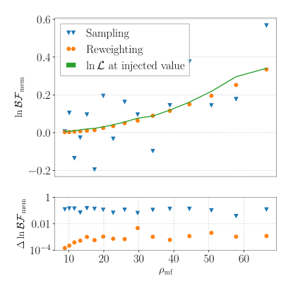
Figure 1: We compare the precision of calculating the Bayes Factors using different techniques for a set different signal-to-noise ratios $\rho_{\mathrm{mf}}$. In the upper panel, we see that using the naive method of dividing the Bayes Factors from eight separate sampling runs (blue triangles), we see a much wider spread away from the fiducial line of likelihood ratios at the injected value (green curve) compared to the Bayes factors we obtained using reweighting (orange squares). In the lower panel, we see that using the reweighting method yields a statistical error that is about $\mathcal{O}(10^{2})$ times smaller.

II.4 Analyzing real events

The analysis of real events mostly follows the prescription in Payne et al. (2019). Initially, we perform inference with the IMRPhenomD model to obtain a “proposal” posterior distribution. Reweighting these posterior samples first with the NRHybSur3dq8, a surrogate waveform model that includes modes $(\ell,m)$ up to $(5,5)$ Varma et al. (2019), yields the Bayes factor for higher-order modes $\text{BF}_{\mathrm{hom}}$, since IMRPhenomD does not contain these modes. Then reweighting with the full NRHybSur3dq8 plus memory model yields the combined higher-order mode plus memory Bayes factor $\text{BF}_{\mathrm{hom+mem}}$. The memory Bayes factor is

$$\text{BF}_{\mathrm{mem}}=\frac{\text{BF}_{\mathrm{hom+mem}}}{\text{BF}_{\mathrm{hom}}}\,$$ (4)

A final issue in the analysis is that NRHybSur3dq8 and IMRPhenomD define the phase $\phi$ and time at coalescence $t_{c}$ differently, and there is no analytic way to map posterior samples between those two definitions. Following Payne et al. (2019), we map the posterior samples from IMRPhenomD to NRHybSur3dq8 by maximizing the waveform overlap in terms of $\phi$ and $t_{c}$ between both models for each posterior sample. The maximum overlap can be quickly found using common optimization techniques. Furthermore, optimizing over the $(\phi,t_{c})$ plane does not require us to evaluate the expensive NRHybSur3dq8 waveform at every step since these are not intrinsic parameters of the waveform. Instead, we produce the waveform once for each posterior sample and project it into the $(\phi,t_{c})$ space as desired. Results using this method analysing the gravitational-wave transient catalog are presented in Section III.

III GWTC-1 Results

We apply the reweighting technique on posterior samples of the first ten binary black hole mergers from the first two LIGO/Virgo observation runs. The results are summarized in Figure 2. The original posterior samples for the proposal run are the same as in Payne et al. (2019). The total $\ln\text{BF}_{\mathrm{mem}}^{\mathrm{tot}}=3.0\times 10^{-3}$ provides no significant support for or against the memory hypothesis. However, this small Bayes factor is expected; we explore why in the subsequent section. We see that even the loudest event in the catalog, GW150914 ($\rho_{\mathrm{mf}}\approx 26$), contributes only weak evidence in favour of the memory hypothesis.

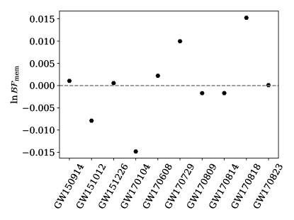
Figure 2: Memory Bayes factors obtained for the first two LIGO/Virgo observation runs. Overall, there is no significant evidence for or against the memory hypothesis.

IV Population study

We construct a simulated population of gravitational-wave events observed by the LIGO/Virgo detector network at design sensitivity so that we can estimate the number of required observations until we reach $\ln\text{BF}\geq 8$. We assume a power-law distribution both in primary mass and in mass ratio as outlined in Abbott et al. (2018). The mass distribution parameters are still poorly constrained given the low number of observations in the first two observing runs. From the posterior distributions in Abbott et al. (2018) we choose parameters that correspond to the points of maximal posterior probability. We choose minimum and maximum black hole masses $m_{\mathrm{min}}=8\,M_{\odot}$ and $m_{\mathrm{max}}=45\,M_{\odot}$ respectively, and use $\alpha=1.5$ and $\beta=3$ as spectral indexes for the primary mass and mass ratio distribution, respectively.

We assume an aligned spin prior distribution Lange et al. (2018), with a maximal allowed spin magnitude of $a_{\mathrm{max}}=0.5$. Higher spins are disfavoured observationally Abbott et al. (2018) and on theoretical grounds Fuller and Ma (2019). At any rate, we do not expect the spin distribution to greatly affect the memory search because the absolute memory amplitude is mostly driven by the overall signal amplitude, which primarily depends on the masses and the luminosity distance of the source. Spin only has an $\mathcal{O}(10\%)$ effect on the memory of a given binary. The remaining extrinsic parameters (inclination, luminosity distance, sky position, time and phase at coalescence, polarisation angle) are chosen using standard priors. We restrict the maximum luminosity distance to $5000\text{\,}\mathrm{Mpc}$ since more distant events are unlikely to be detected.

We randomly sample parameters from the distributions in intrinsic and extrinsic parameters. However, the LIGO/Virgo detector network will only be able to actually detect a fraction of all occurring binary black hole mergers in the Universe. We therefore only keep events with a matched filter signal-to-noise ratio greater than 12 in the network and/or greater than 8 in any single detector. Otherwise, the event is considered to be undetected.

Following the steps outlined Section II.4, we obtain Bayes factors for each event. In practice, this works reliably up to a matched filter signal-to-noise ratio $\rho_{\mathrm{mf}}\approx 32$, i.e. we recover the injected parameters and obtain an acceptable number of effective samples after reweighting Payne et al. (2019). At higher $\rho_{\mathrm{mf}}$, systematic differences between IMRPhenomD and NRHybSur3dq8 can cause the inference runs to converge to non-overlapping regions in parameter space. In those cases the reweighting technique using the IMRPhenomD model becomes invalid if the posterior does not extend over the true value of the injected NRHybSur3dq8 data. We resolve this issue by performing inference with the NRHybSur3dq8 model directly and then reweighting the posterior samples to the NRHybSur3dq8 plus memory model. Since sampling with NRHybSur3dq8 is of far greater computational expense, we do not extend its use to the $\rho_{\mathrm{mf}}<32$ events, which comprise $92.5\%$ of all events in our population set. Instead, we use the reweighting technique with IMRPhenomD proposal distribution for these events.

We perform the analysis on a set of 2000 events and re-run inference until each combined posterior has at least 20 effective samples. By requiring this number of effective samples, we ensure that the samples are reasonably closely converged to the injected value. Otherwise, the weights would wildly diverge and the number of effective samples would hence always be close to unity.

We display the results of our population study in Figure 3 (blue curve). The population passes $\ln\text{BF}>8$ after about 2000 events. We also simulate many more events for which we estimate the Bayes factor by using the likelihood ratio at the injected values (gray curves). Using this much larger population, we estimate the required number of events to reach $\ln\text{BF}\geq 8$ to be $1830^{+1730}_{-1100}$ at the $90\%$ confidence level. Although this study likely overestimates the Bayes factors since it implicitly assumes that we can always break the $(\phi,\psi)$ degeneracy, we still consider this to be a good approximation since most support for memory comes from very few events with exceptionally high signal-to-noise ratios.

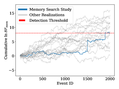
Figure 3: Cumulative memory Bayes factors obtained for a set of 2000 injections. The blue curve shows the recovered Bayes Factors using nested sampling and reweighting. The dashed red line displays the threshold for detection. The gray lines show a set of realizations using the the likelihood ratio at the injected parameters.

V Conclusion and Outlook

We have found a combined $\ln\text{BF}=0.003$ for the existence of memory in the gravitational waves from the ten binary black holes observed by LIGO/Virgo in their first two observing runs. We have shown that we need $1830^{+1730}_{-1100}$ events to reach $\ln\text{BF}=8$, which can be considered to be a detection of memory Lasky et al. (2016). This is likely to take place in the early days of A+/Virgo+, when observatories will be detecting ${\cal O}(10)$ events a day. Adding KAGRA Somiya (2012) and LIGO-India Unnikrishnan (2013) to the network will further reduce the time until memory is detected. Furthermore, reducing noise at low frequencies has also been shown to substantially decrease the number of detections required Yu et al. (2018), reducing the time to detection by a factor of $~{}3$. Once memory is observed, it may be possible to use it to probe the nature of black holes and to look for physics beyond general relativity; see, e.g., Yang and Martynov (2018).

We have shown how recent innovations, such as memory waveforms Talbot et al. (2018), and waveforms with higher-order modes enable us to know the sign of the memory, despite the computational challenges. By introducing likelihood reweighting we reduce the stochastic sampling error by a factor of $\mathcal{O}(10^{2})$, which is equivalent in terms of error reduction to an increase in sampling time by $\mathcal{O}(10^{4})$. Additionally, we show that by fine-tuning sampling parameters we can obtain confident measures of the Bayes factor within one week of computation time even if we have to use costly waveform models.

VI Acknowledgements

We would like to thank Robert Wald for helpful comments. We would also like to thank Ethan Payne for kindly providing his posterior samples and helpful conversations. This work is supported through Australian Research Council (ARC) Centre of Excellence CE170100004. PDL is supported through ARC Future Fellowship FT160100112 and ARC Discovery Project DP180103155. ET is supported through ARC Future Fellowship FT150100281 and CE170100004. This is LIGO Document No. DCC P1900346.

References

- Aasi et al. (2015) J. Aasi et al., Class. Quantum Grav 32, 074001 (2015).
- Acernese et al. (2015) F. Acernese et al., Classical and Quantum Gravity 32, 024001 (2015).
- Abbott et al. (2019a) B. P. Abbott et al., \prx 9, 031040 (2019a).
- Abbott et al. (2016) B. P. Abbott et al., Phys. Rev. Lett. 116, 221101 (2016).
- Abbott et al. (2019b) B. P. Abbott et al., Phys. Rev. Lett. 123, 011102 (2019b).
- Abbott et al. (2019) B. P. Abbott et al., (2019), arXiv:1903.04467 .
- Ghosh et al. (2016) A. Ghosh et al., Phys. Rev. D 94, 021101 (2016).
- Zel’dovich, Ya. and Polnarev (1974) B. Zel’dovich, Ya. and A. G. Polnarev, Soviet Ast. 18, 17 (1974).
- Braginsky and Thorne (1987) V. B. Braginsky and K. S. Thorne, Nature 327, 123 (1987).
- Thorne (1992) K. S. Thorne, Phys. Rev. D 45, 520 (1992).
- Demetrios Christodoulou (1991) Demetrios Christodoulou, Phys. Rev. Lett. 67, 1486 (1991).
- Lasky et al. (2016) P. D. Lasky et al., Phys. Rev. Lett. 117, 061102 (2016).
- Johnson et al. (2019) A. D. Johnson et al., Phys. Rev. D 99, 044045 (2019).
- Abbott et al. (2017) B. P. Abbott et al., Class. Quantum Grav. 34, 044001 (2017).
- Punturo et al. (2010) M. Punturo et al., Class. Quantum Grav. 27, 194002 (2010).
- Islo et al. (2019) K. Islo et al., (2019), arXiv:1906.11936 .
- Aasi et al. (2015) J. Aasi et al., Class. Quantum Grav. 32, 074001 (2015).
- Acernese et al. (2014) F. Acernese et al., Class. Quantum Grav. 32, 024001 (2014).
- Yu et al. (2018) H. Yu et al., (2018), arXiv:1712.05417 .
- Van Haasteren and Levin (2010) R. Van Haasteren and Y. Levin, MNRAS 401, 2372 (2010).
- Cordes and Jenet (2012) J. M. Cordes and F. A. Jenet, ApJ 752, 54 (2012).
- Madison et al. (2014) D. R. Madison et al., ApJ 788, 141 (2014).
- Wang et al. (2015) J. B. Wang et al., MNRAS 446, 1657 (2015).
- Arzoumanian et al. (2015) Z. Arzoumanian et al., ApJ 810, 150 (2015).
- Aggarwal et al. (2019) K. Aggarwal et al., (2019), arXiv:1911.08488 .
- Dewdney et al. (2009) P. Dewdney et al., Proceedings of the Institute of Electrical and Electronics Engineers IEEE 97, 1482 (2009).
- Kurita and Nakano (2016) Y. Kurita and H. Nakano, Phys. Rev. D 93, 023508 (2016).
- Greene (2012) J. E. Greene, Nature Comms. 3, 1304 (2012).
- Nakamura et al. (1997) T. Nakamura et al., ApJ 487, L139 (1997).
- Damour and Vilenkin (2000) T. Damour and A. Vilenkin, Phys. Rev. Lett. 85, 3761 (2000).
- McNeill et al. (2017) L. O. McNeill et al., Phys. Rev. Lett. 118, 181103 (2017).
- Bieri et al. (2016) L. Bieri et al., Phys. Rev. D 94, 064040 (2016).
- Bieri et al. (2017) L. Bieri et al., Class. Quantum Grav. 34, 215002 (2017).
- Strominger and Zhiboedov (2016) A. Strominger and A. Zhiboedov, Journal of High Energy Physics 2016, 86 (2016).
- Hawking et al. (2016) S. W. Hawking et al., Phys. Rev. Lett. 116, 231301 (2016).
- Kapec et al. (2017) D. Kapec et al., Class. Quantum Grav. 34, 165007 (2017).
- Blackman et al. (2015) J. Blackman et al., Phys. Rev. Lett. 115, 121102 (2015).
- Varma et al. (2019) V. Varma et al., Phys. Rev. D 99, 064045 (2019).
- Favata (2010) M. Favata, Class. Quantum Grav. 27 (2010).
- Favata (2009a) M. Favata, ApJ 696, 20 (2009a), 0902.3660 .
- Favata (2009b) M. Favata, Phys. Rev. D 80, 1 (2009b), 0812.0069 .
- Talbot et al. (2018) C. Talbot et al., (2018), arXiv:arXiv:1807.00990v1 .
- Khan et al. (2016) S. Khan et al., Phys. Rev. D 93, 044007 (2016).
- Thrane and Talbot (2019) E. Thrane and C. Talbot, PASA 36, e010 (2019).
- Skilling (2004) J. Skilling, in American Institute of Physics Conference Series, Vol. 735, edited by R. Fischer, R. Preuss, and U. V. Toussaint (2004) pp. 395–405.
- Feroz and Hobson (2008) F. Feroz and M. P. Hobson, MNRAS 384, 449 (2008).
- Speagle (2019) J. S. Speagle, (2019), arXiv:1904.02180 .
- Payne et al. (2019) E. Payne et al., (2019), arXiv:1905.05477 .
- Romero-Shaw et al. (2019) I. M. Romero-Shaw et al., (2019), arXiv:1909.05466 .
- Ashton et al. (2019) G. Ashton et al., ApJS 241, 27 (2019).
- Chopin and Robert (2010) N. Chopin and C. P. Robert, Biometrika 97, 741 (2010).
- Abbott et al. (2018) B. P. Abbott et al., (2018), arXiv:1811.12940 .
- Lange et al. (2018) J. Lange et al., (2018), arXiv:1805.10457 .
- Fuller and Ma (2019) J. Fuller and L. Ma, ApJ 881, L1 (2019).
- Somiya (2012) K. Somiya, Classical and Quantum Gravity 29, 124007 (2012).
- Unnikrishnan (2013) C. S. Unnikrishnan, International Journal of Modern Physics D 22, 1341010 (2013).
- Yang and Martynov (2018) H. Yang and D. Martynov, (2018), arXiv:1803.02429 .