Maximum likelihood estimators for scaled mutation rates in an equilibrium mutation-drift model

Abstract

The stationary sampling distribution of a neutral decoupled Moran or Wright-Fisher diffusion with neutral mutations is known to first order for a general rate matrix with small but otherwise unconstrained mutation rates. Using this distribution as a starting point we derive results for maximum likelihood estimates of scaled mutation rates from site frequency data under three model assumptions: a twelve-parameter general rate matrix, a nine-parameter reversible rate matrix, and a six-parameter strand-symmetric rate matrix. The site frequency spectrum is assumed to be sampled from a fixed size population in equilibrium, and to consist of allele frequency data at a large number of unlinked sites evolving with a common mutation rate matrix without selective bias. We correct an error in a previous treatment of the same problem Burden and Tang [7] affecting the estimators for the general and strand-symmetric rate matrices. The method is applied to a biological dataset consisting of a site frequency spectrum extracted from short autosomal introns in a sample of Drosophila melanogaster individuals.

1 Introduction

A significant obstacle to inferring evolutionary parameters from allele frequency data is the paucity of accurate solutions to well-established stochastic population genetics models [25]. For instance, it should, in principle, be possible to infer scaled mutation rates from population allele frequencies observed in unlinked neutral genomic sites whose genealogies are independent due to the effects of recombination [19]. As a minimal requirement, such inference requires solution of, say, a Wright-Fisher or Moran model with mutations, typically formulated in the diffusion limit. For the case of a stationary bi-allelic system, Vogl [26] has demonstrated that this is feasible as the stationary distribution in the diffusion limit of the mutation-drift model is known to be a beta distribution and the corresponding sampling distribution is beta-binomial. This analysis has been extended to include a bi-allelic mutation-drift system with directional selection [27].

Inference of the complete $4\times 4$ genomic mutation rate matrix from allele frequency data requires solution of a multi-allele mutation-drift model. There is no known exact solution to the diffusion limit of the multi-allele mutation-drift model except for the case of parent-independent mutations, for which the stationary solution is known to be a Dirichlet distribution [29, p394], and the corresponding sampling distribution is Dirichlet-multinomial. However, a recent extensive study of the moments of allele distributions under various model rate matrices [23] has demonstrated the shortcomings of the Dirichlet approximation in more general settings than the biologically unrealistic parent independent model.

The scaled mutation rate in the diffusion limit, which is often termed $\theta$, is essentially the product of a per base substitution mutation rate per nucleotide site per generation ($u$) and an effective population size ($N$). In a study of silent states in protein-coding genes Lynch et al. [17, Fig. 3b] observe that $u$ decreases from about $\sim 10^{-8}$ to about $\sim 10^{-10}$ as $N$ ranges from $\sim 10^{4}$ to $\sim 10^{8}$ in eukaryotes. This corresponds to scaled mutation rates which are $<10^{-2}$. A promising approach therefore is to consider small-$\theta$ approximations either to solutions of the multi-allele mutation-drift model, or to the model itself.

The stationary solution to the multi-allele mutation-drift diffusion with an arbitrary mutation rate matrix has been obtained to first order in $\theta$ [6] by solving the forward Kolmogorov equation. The corresponding sampling distribution has been determined by Burden and Tang [7] and verified by Burden and Griffiths [4] using a coalescent approach. The identical sampling distribution has been derived independently by Schrempf and Hobolth [21] from a boundary-mutation model [27] based on the decoupled Moran model.

The purpose of the current paper is to explore the process of inferring a complete neutral mutation rate matrix from a spectrum of observed allele frequencies at independently evolving sites from the stationary sampling distribution. Our starting point is the small-$\theta$ sampling distribution described above. We obtain maximum likelihood (ML) estimates which can be efficiently computed under assumptions of (i) a general unconstrained rate matrix, (ii) a reversible rate matrix, and (iii) a strand-symmetric rate matrix. In each case we construct combinations of rate matrix parameters, which have unbiased ML estimators, and determine which parameters necessarily have biased ML estimators. We also correct an error in Burden and Tang [7] in which the ML estimator of the rate matrix for a general unconstrained rate matrix is incorrectly stated.

The format of the paper is as follows: In Section 2 the multi-allele mutation-drift diffusion is defined and the ${\mathcal{O}}(\theta)$ stationary sampling distribution is stated. The statement of the inference problem and a description of the form of the multi-allele frequency dataset for an effective haploid sample size of $M$ individuals at a total of $L$ sites (or loci) is described in Section 3, together with a brief summary of how ML estimation will be implemented in subsequent sections. Section 4 gives a reparametrization of the rate matrix in a form suitable for analysing reversible and non-reversible rate matrices. Derivation of ML estimates for the case of a general unconstrained rate matrix and for the case of a rate matrix constrained to be reversible are given in Section 5. The strand-symmetric case is covered in Section 6. The theory is applied to a dataset extracted from short autosomal introns of 197 Drosophila melanogaster individuals at 218,942 genomic sites in Section 7, and simulations exploring the accuracy and applicability of the small-$\theta$ approximation can be found in Section 8. Conclusions are drawn in Section 9, while an Appendix is devoted to technical details of numerical optimisation.

2 Stationary sampling distribution for a general rate matrix

We will begin our derivations by considering a $K$-allele neutral decoupled Moran model [1, 12, 28] or haploid Wright-Fisher model [11, p55] with scaled rate matrix

$$Q_{ij}=\begin{cases}N(u_{ij}-\delta_{ij})&\text{(decoupled Moran)}\\ 2N(u_{ij}-\delta_{ij})&\text{(Wright-Fisher)},\end{cases}$$ (1)

where $N$ is the haploid (effective) population size and $u_{ij}$ are the per generation mutation rates. The diffusion limit of this process is defined by the simultaneous limits $N\rightarrow\infty$ and $u_{ij}\rightarrow\delta_{ij}$ for fixed $Q_{ij}$ and can be described by the backward generator

$$\frac{1}{2}\sum_{i,j=1}^{K}x_{i}(\delta_{ij}-x_{j})\frac{\partial^{2}}{\partial x_{i}\partial x_{j}}+\frac{1}{2}\sum_{i=1}^{K}Q_{ij}x_{j}\frac{\partial}{\partial x_{i}}.$$ (2)

where $x_{i}$ and $x_{j}$ denote the respective allele frequencies.

In its most general form the $K\times K$ rate matrix $\mathbf{Q}$ is constrained by

$$Q_{ij}\geq 0,\quad\text{for }i\neq j;\qquad\sum_{j=1}^{K}Q_{ij}=0,$$ (3)

implying that $K(K-1)$ parameters are required to specify $\mathbf{Q}$. Let us assume that $\mathbf{Q}$ has a unique stationary state $\pi^{\rm T}=(\pi_{1}\ldots\pi_{K})$ satisfying

$$\pi_{i}\geq 0,\quad\sum_{i=1}^{K}\pi_{i}=1,\quad\sum_{i=1}^{K}\pi_{i}Q_{ij}=0.$$ (4)

A sufficient condition for a unique $\pi^{\rm T}$ to exist is $Q_{ij}>0$ for all $i\neq j$. One would expect this to include any biologically realistic model.

Suppose we further assume small scaled mutation rates, that is, assume the off-diagonal elements of $\mathbf{Q}$ to be ${\cal O}(\theta)$ for some small parameter $\theta$. The sampling distribution for a finite sample of $M$ individuals randomly and independently drawn from the population of size $N$ has been obtained to first order in $\theta$ by Burden and Tang [7, Eq. (35)] from an approximate solution to the forward Kolmogorov equation corresponding to the generator in Eq. (2) and by Burden and Griffiths [4, Theorem 1] from the coalescent. An identical distribution has also been given by Schrempf and Hobolth [21] using the boundary-mutation model as a starting point. Let

$$\mathbf{Y}=(Y_{1},\ldots,Y_{K}),\qquad\sum_{i=1}^{K}Y_{i}=M,$$ (5)

be the occupancy of alleles in a population sample of size $M$, assuming stationarity. Then the stationary sampling distribution is, to first order in $\theta$,

$$\Pr(\mathbf{Y}=\mathbf{y}\mid M,\mathbf{Q})=\begin{cases}\displaystyle\pi_{i}\left(1-H_{M-1}\sum_{j\neq i}Q_{ij}\right)+\mathcal{O}(\theta^{2}),&y_{i}=M,y_{j\neq i}=0;\\ \\ \displaystyle{\frac{\pi_{i}Q_{ij}}{y_{j}}+\frac{\pi_{j}Q_{ji}}{y_{i}}}+\mathcal{O}(\theta^{2}),&1\leq y_{i},y_{j\neq i}\leq M-1\\ &\text{ and }y_{i}+y_{j}=M\,;\\ \\ \mathcal{O}(\theta^{2}),&y_{i},y_{j},y_{k}>0\text{ for distinct $i$, $j$, $k$,}\end{cases}$$ (6)

where

$$H_{M-1}=\sum_{y=1}^{M-1}\frac{1}{y}.$$ (7)

This distribution is a generalisation of special cases corresponding to situations where the stationary distribution of the neutral Moran or Wright-Fisher diffusion is known exactly. The corresponding 2-allele case is quoted in Vogl [26, Eq. (29)], and the case of multi-allelic parent-independent rate matrix is given in RoyChoudhury and Wakeley [20, Eq. (10)]. Both of these special cases correspond to reversible rate matrices, for which $\pi_{i}Q_{ij}=\pi_{j}Q_{ji}$, leading to simplification of the second line in Eq. (6).

3 Site frequency data

Our aim is to estimate the scaled mutation rate matrix $\mathbf{Q}$ from a dataset in the form of a site frequency spectrum obtained by sampling $L$ independent neutrally evolving loci within multiple alignments of $M$ genomes. The obvious application is to the genomic alphabet $\{A,T,G,C\}$ of $K=4$ letters, with the loci being neutral genomic sites such as fourfold degenerate sites within codons or short intron sites [27]. Such a dataset can be achieved in principle from a sample of $M/2$ diploid, monoecious individuals, with the sites chosen to be sufficiently separated so as to have independent coalescent trees due to recombination. In terms of the allele occupancy counts defined by Eq. (5), set

$$\begin{split}L_{i}&=\text{the number of sites with $Y_{i}=M$, $Y_{j\neq i}=0$};\\ L_{ij}(y)&=\text{the number of sites with $Y_{i}=y$, $Y_{j\neq i}=M-y$, $Y_{k\neq i,j}=0$};\\ \end{split}$$ (8)

for $1\leq i,j,k\leq K$ and $y=1,\ldots M-1$. Also define

$$\begin{split}L_{ij}&=\sum_{y=1}^{M-1}L_{ij}(y);\\ L_{\rm P}&=\sum_{1\leq i<j\leq K}L_{ij}.\end{split}$$ (9)

Thus $L_{i}$ counts the number of non-segregating sites with allele $i$, $L_{ij}$ counts the number of bi-allelic sites with alleles $i$ and $j$, and $L_{\rm P}$ counts the total number of bi-allelic sites. Since Eq. (6) implies that tri-allelic, tetra-allelic, etc. sites only occur with probability ${\mathcal{O}}(\theta^{2})$, we further assume that all sites are either non-segregating (with probability ${\mathcal{O}}(1)$) or bi-allelic (with probability ${\mathcal{O}}(\theta)$), and hence the total number of sites is

$$L=\sum_{i}L_{i}+L_{\rm P}.$$ (10)

Note that under the model defined by the distribution Eq. (6), $L_{i}$ and $L_{ij}(y)$ are random variables, whereas $L$ is set by experimental design and is not a random variable.

Let the vector of random site counts

$$\mathbf{L}=(L_{i},L_{ij}(y)),\quad 1\leq i\leq K;\,1\leq j<j\leq K;\,y=1,\ldots,M-1,$$ (11)

listed in Eq. (8) take observed values $\bm{\ell}=(l_{i},l_{ij}(y))$. To first order in $\theta$, we obtain from Eq. (6) the likelihood function

$${\cal L}(\mathbf{Q}\mid\bm{\ell}) := \Pr\left(\mathbf{L}=\bf{\bm{\ell}}\mid\mathbf{Q}\right)$$ (12)

$$= \frac{L!}{(\prod_{i}l_{i}!)(\prod_{i<j}\prod_{y=1}^{M-1}l_{ij}(y)!)}$$

$$\quad\times\prod_{i=1}^{K}\left\{\pi_{i}\left(1-H_{M-1}\sum_{j\neq i}Q_{ij}\right)\right\}^{l_{i}}$$

$$\quad\times\prod_{1\leq i<j\leq K}\prod_{y=1}^{M-1}\left\{{\frac{\pi_{i}Q_{ij}}{M-y}+\frac{\pi_{j}Q_{ji}}{y}}\right\}^{l_{ij}(y)}.$$

Note that this is a multinomial distribution in $\mathbf{L}$.

The general form of a multinomial distribution is

$$\mbox{$\rm{Prob}$\,}(\mathbf{L}=\bm{\ell})=\frac{{\color[rgb]{0,0,0}L!}}{\prod_{\alpha}l_{\alpha}!}\prod_{\alpha}p_{\alpha}^{l_{\alpha}}={L\choose\bm{\ell}}\prod_{\alpha}p_{\alpha}^{l_{\alpha}},$$ (13)

where $\sum_{\alpha=1}^{n}l_{\alpha}=L$ for a fixed number of categories $n$ and parameters $p_{\alpha}$, with $\alpha=1,\ldots,n$ constrained by

$$p_{\alpha}>0,\qquad\sum_{\alpha=1}^{n}p_{\alpha}=1.$$ (14)

In general, $E(L_{\alpha})=Lp_{\alpha}$, so the random variables

$$\hat{p}_{\alpha}=\frac{L_{\alpha}}{L},$$ (15)

are unbiased estimators of $p_{\alpha}$. By writing Eq. (13) in the canonical form

$$\mbox{$\rm{Prob}$\,}(\mathbf{L}=\bm{\ell})={L\choose\bm{\ell}}p_{n}^{L}\exp\left(\sum_{\beta=1}^{n-1}l_{\beta}\log\frac{p_{\beta}}{p_{n}}\right),$$ (16)

one sees that the multinomial with fixed $L$ and unknown $p_{\alpha}$ constitutes an exponential family of distributions with sufficient statistics $L_{1},\ldots,L_{n-1}$ (sufficiency can easily be seen via the Neyman factorisation theorem  [13, pp 318, 341]). Essentially this means that all the information from the data needed to construct any estimator of $p_{\alpha}$ is known through $L_{1},\ldots,L_{n-1}$; the probability of the data given $L_{1},\ldots,L_{n-1}$ is therefore independent of $p_{\alpha}$ itself.

Furthermore, if Eq. (14) are the only constraints on the $p_{\alpha}$, then $L_{1},\ldots,L_{n-1}$ are a minimal complete set of sufficient statistics (completeness via Definition 3.19 of Keener [14, p 50]) and the natural parameter space maps identifiably onto that of the estimators. The theory of exponential families tells us that $\hat{p_{\alpha}}$ defined by Eq. (15) are in fact uniformly minimum variance unbiased estimators. This can be shown by application of the Rao-Blackwell theorem as shown in Theorem 4.4 of Keener [14, p 62]. The argument via completeness in the referenced proof is often given separately as the Lehmann-Sheffe theorem, which can also be verified with a straightforward calculation using Lagrange multipliers. This shows that these estimators are also unique ML estimators. We will refer to such multinomials as being flat.

However, the analogous parameters in Eq. (12) are functions of elements of the rate matrix $\mathbf{Q}$, which are themselves subject to nontrivial constraints via Eqs. (3) and (4). In this case, the number of independent parameters is less than the number of sufficient statistics and the exponential family is said to be curved [14, Chapter 5]. Many of the standard results pertaining to flat exponential families do not generalise to curved exponential families. Importantly for our case, the estimators defined by Eq. (15) are still unbiased but, in general, are not ML estimators of $p_{\alpha}$.

In the following sections we explore the problem of determining ML estimators under various model restrictions on the rate matrix $\mathbf{Q}$. In most cases exact analytic formulae for ML estimates of the complete set of parameters are intractable. However, by judicious use of reparametrization we are able exploit the Neyman factorisation theorem [13, pp 318, 341] to factor Eq. (12) into (i) flat marginal multinomials, from which minimum variance unbiased ML estimators can be obtained for certain combinations of parameters, and (ii) a quotient depending on the remaining parameters, for which ML estimators can be determined numerically. We begin by introducing a reparametrization of the rate matrix into reversible and non-reversible parts, which will enable us to specify a convenient minimal set of independent parameters of the general rate matrix $\mathbf{Q}$.

4 Reparametrization of the rate matrix

Recall the defining properties of the rate matrix $\mathbf{Q}$ and its stationary distribution $\mathbf{\pi^{T}}$, Eqs. (3) and (4).

Define the parameters

$$C_{ij}=\tfrac{1}{2}(\pi_{i}Q_{ij}+\pi_{j}Q_{ji}),\qquad\Phi_{ij}=\tfrac{1}{2}(\pi_{i}Q_{ij}-\pi_{j}Q_{ji}),$$ (17)

for $i,j=1,\ldots,K$. One easily checks that

$$Q_{ij}=(C_{ij}+\Phi_{ij})/\pi_{i},$$ (18)

where the first term is the reversible part of the rate matrix, $Q_{ij}^{\rm GTR}=C_{ij}/\pi_{i}$, and the second term, $Q_{ij}^{\rm flux}=\Phi_{ij}/\pi_{i}$ represents a flux $\Phi_{ij}$ of probability per unit time from allele $i$ to allele $j$ [7].

It follows that $C_{ij}$ are the elements of a symmetric $K\times K$ matrix satisfying $\sum_{j=1}^{K}C_{ij}=0$, and that $\Phi_{ij}$ are the elements of an antisymmetric $K\times K$ matrix satisfying $\sum_{j=1}^{K}\Phi_{ij}=0$. This last constraint is a statement that fluxes of probability out of any allele to the remaining $K-1$ alleles must be zero.

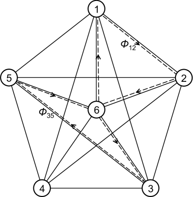
Figure 1: Probability fluxes through the edges of the simplex spanned by $K=6$ alleles. The independent $\Phi_{ij}$ for all $1\leq i<j\leq K-1$ contribute probability fluxes around paths $K\rightarrow i\rightarrow j\rightarrow K$ as shown for $\Phi_{12}$ and $\Phi_{35}$. The remaining radial fluxes $\Phi_{iK}$ for $i\neq K$ are obtained by summing fluxes from all such triangular paths passing through $i$ and $K$.

Clearly the stationary distribution $\pi_{i}$ contains $K-1$ independent degrees of freedom, and the parameters $C_{ij}$ contribute $\frac{1}{2}K(K-1)$ independent degrees of freedom. To understand the number of independent elements of $\Phi_{ij}$, consider Fig. 1 illustrating the case $K=6$. Placing the $K$-th allele at the centre of the diagram, we observe that the $\frac{1}{2}(K-1)(K-2)$ closed paths $K\rightarrow i\rightarrow j\rightarrow K$ for $1\leq i<j\leq K-1$ define independent fluxes $\Phi_{ij}$, and that the flux along any radial edge $i\rightarrow K$ for $1\leq i\leq K-1$ can be obtained by conserving flux at the vertex $i$. To summarise, the general rate matrix $\mathbf{Q}$ can be parameterised using the following minimal set of parameters:

$$\begin{array}[]{lrr}\pi_{i},&i=1,\ldots,K-1:&K-1\mbox{ parameters};\\ C_{ij},&1\leq i<j\leq K:&\tfrac{1}{2}K(K-1)\mbox{ parameters};\\ \Phi_{ij},&1\leq i<j\leq K-1:&\tfrac{1}{2}(K-1)(K-2)\mbox{ parameters},\end{array}$$ (19)

with the remaining, dependent parameters given by

$$\begin{split}\pi_{K}&=\sum_{i=1}^{K-1}\pi_{i},\\ C_{ji}&=C_{ij},\quad 1\leq i<j\leq K,\\ C_{ii}&=\sum_{j\neq i}C_{ij}\quad 1\leq i\leq K,\\ \Phi_{ji}&=-\Phi_{ij},\quad 1\leq i<j<K,\\ \Phi_{iK}&=-\Phi_{Ki}=\sum_{j=1}^{i-1}\Phi_{ji}-\sum_{j=i+1}^{K-1}\Phi_{ij},\quad 1\leq i\leq K-1.\end{split}$$ (20)

The total number of independent parameters is $K(K-1)$, as required.

5 Maximum likelihood estimates

We can now use the theory from Section 3 to discuss the properties of ML estimators of the (reparametrized) rate matrix in three biologically relevant scenarios.

5.1 $K=2$ alleles

Because the $2\times 2$ rate matrix for the bi-allelic mutation-drift model is necessarily reversible, there are no probability fluxes and therefore only two independent parameters, $\pi_{1}$ and $C_{12}$. The ML estimators of these parameters were derived by Vogl [26]. Here we re-derive the estimators in a way which readily generalises to both the general $K$-allele model and the reversible $K$-allele model.

From Eqs. (12), (18) and (20) we have

$$\Pr\left(L_{1}=l_{1},L_{2}=l_{2},L_{12}(y)=l_{12}(y)\mid\pi_{1},C_{12}\right)$$ (21)

$$= g(l_{1},l_{2},l_{12};\pi_{1},C_{12})\times h(\vec{l}_{12}),$$

where

$$g(l_{1},l_{2},l_{12};\pi_{1},C_{12})$$ (22)

$$= \frac{L!}{l_{1}!l_{2}!l_{12}!}(\pi_{1}-H_{M-1}C_{12})^{l_{1}}(1-\pi_{1}-H_{M-1}C_{12})^{l_{2}}(2H_{M-1}C_{12})^{l_{12}},$$

$$h(\vec{l}_{12})=\frac{1}{(2H_{M-1})^{l_{12}}}\frac{l_{12}!}{\prod_{y=1}^{M-1}l_{12}(y)!}\prod_{y=1}^{M-1}\left(\frac{1}{M-y}+\frac{1}{y}\right)^{l_{12}(y)},$$ (23)

and

$$\vec{l}_{12}=(l_{12}(1),\ldots,l_{12}(M-1)).$$ (24)

Since $h(\vec{l}_{12})$ does not depend on $\pi_{1}$ or $C_{12}$, the Neyman factorisation theorem for multiple parameters [13, pp 341] necessitates that $L_{1},L_{2}$ and $L_{12}$ are sufficient statistics for estimating $\pi_{1}$ and $C_{12}$. Then, since

$$\sum_{\{\vec{l}_{12}:\,\sum_{y}l_{12}(y)=l_{12}\}}h(\vec{l}_{12})=\left\{\frac{1}{2H_{M-1}}\sum_{y=1}^{M-1}\left(\frac{1}{M-y}+\frac{1}{y}\right)\right\}^{l_{12}}=1,$$ (25)

the marginal probability in $L_{1},L_{2}$ and $L_{12}$ is simply

$$\Pr\left(L_{1}=l_{1},L_{2}=l_{2},L_{12}=l_{12}\mid\pi_{1},C_{12}\right)=g(l_{1},l_{2},l_{12};\pi_{1},C_{12}).$$ (26)

Eq. (22) is a flat family of trinomial distributions with two independent parameters. It follows from Eq. (15) and the discussion following Eq. (16) that $\hat{p}_{1}=L_{1}/L$ and $\hat{p}_{12}=L_{12}/L$ are minimum variance, unbiased, ML estimators of $p_{1}:=\pi_{1}-H_{M-1}C_{12}$ and $p_{12}:=2H_{M-1}C_{12}$ respectively. The required ML estimators are then

$$\hat{C}_{12}=\frac{L_{12}}{2LH_{M-1}},\quad\hat{\pi}_{1}=\frac{L_{1}+\frac{1}{2}L_{12}}{L},$$ (27)

agreeing with Vogl [26, Eqs. (36) and (37)]. By linearity they are also unbiased.

5.2 General $K$-allele model

Returning to the $K$-allele mutation-drift model for a general $K\times K$ rate matrix, we have, from Eqs. (12), (18) and the properties of $C_{ij}$ and $\Phi_{ij}$,

$$\Pr\left(\mathbf{L}=\bm{\ell}\mid\pi_{i},C_{ij},\Phi_{ij}\right)$$ (28)

$$= \frac{L!}{(\prod_{i}l_{i}!)(\prod_{i<j}\prod_{y=1}^{M-1}l_{ij}(y)!)}\prod_{i=1}^{K}\left(\pi_{i}-H_{M-1}\sum_{j\neq i}C_{ij}\right)^{l_{i}}$$

$$\quad\times\prod_{1\leq i<j\leq K}\prod_{y=1}^{M-1}\left\{C_{ij}\left({\frac{1}{M-y}+\frac{1}{y}}\right)+\Phi_{ij}\left({\frac{1}{M-y}-\frac{1}{y}}\right)\right\}^{l_{ij}(y)},$$

where the vector $\mathbf{L}$ of random variables represents the complete set of counts in Eq. (11).

Our aim is to choose a parametrization that will enable us to exploit the Neyman factorisation theorem. To this end we define

$$\begin{split}C&=\sum_{1\leq i<j\leq K}C_{ij};\\ \pi_{i}^{\prime}&=\frac{\pi_{i}-H_{M-1}\sum_{j\neq i}C_{ij}}{1-2H_{M-1}C},\quad i=1,\ldots,K;\\ c_{ij}&=\frac{C_{ij}}{C},\quad i,j=1,\ldots,K;\\ \phi_{ij}&=\frac{\Phi_{ij}}{C},\quad i,j=1,\ldots,K.\end{split}$$ (29)

One easily checks that $\sum_{i=1}^{K}\pi_{i}^{\prime}=1$, and therefore $K-1$ of $\pi_{i}^{\prime}$ are independent; that $\sum_{i<j}c_{ij}=1$, and therefore $\frac{1}{2}K(K-1)-1$ of the $c_{ij}$ are independent; and that, by analogy with the $\Phi_{ij}$, there are $\frac{1}{2}(K-1)(K-2)$ independent rescaled fluxes $\phi_{ij}$. Together with $C$ this gives a total of $K(K-1)$ independent parameters, as required. In the following we choose for the set of independent parameters

$$\{\pi_{1}^{\prime},\ldots,\pi_{K-1}^{\prime},C\}\cup\left(\{c_{ij}:1\leq i<j\leq K\}\backslash\{c_{K-1,K}\}\right)\cup\{\phi_{ij}:1\leq i<j\leq{K-1}\}.$$ (30)

The remaining, dependent, parameters in Eq. (29) are then defined as

$$\begin{split}c_{K-1,K}&=1-\sum_{1\leq i<j\leq K-1}c_{ij}-\sum_{i=1}^{K-2}c_{iK},\\ \phi_{iK}&=\sum_{j=1}^{i-1}\phi_{ji}-\sum_{j=i+1}^{K-1}\phi_{ij},\quad 1\leq i\leq K-1.\end{split}$$ (31)

Let us further define the vector of bi-allelic counts as

$$\bm{\ell}_{\rm P}=(l_{ij}(y)),\qquad 1\leq i<j\leq K,\,y=1,\ldots,M-1,$$ (32)

and the sum

$$l_{\rm P}=\sum_{i<j}\sum_{y}l_{ij}(y)$$ (33)

This reparametrization gives Eq. (28) as

$$\Pr\left(\mathbf{L}=\bm{\ell}\mid\pi_{i}^{\prime},C,c_{ij},\phi_{ij}\right)$$ (34)

$$= g(l_{1},\ldots,l_{K},l_{\rm P};\pi_{1}^{\prime},\ldots,\pi_{K-1}^{\prime},C)\times h(\bm{\ell}_{\rm P};c_{ij},\phi_{ij}),$$

where

$$g(l_{1},\ldots,l_{K},l_{\rm P};\pi_{1}^{\prime},\ldots,\pi_{K-1}^{\prime},C)$$ (35)

$$= \frac{L!}{(\prod_{i=1}^{K}{\color[rgb]{0,0,0}l_{i}!})l_{\rm P}!}\left(\prod_{i=1}^{K-1}\left\{(1-2H_{M-1}C)\pi_{i}^{\prime}\right\}^{l_{i}}\right)$$

$$\qquad\times\left\{(1-2H_{M-1}C)\left(1-\sum_{i=1}^{K-1}\pi_{i}^{\prime}\right)\right\}^{l_{K}}(2H_{M-1}C)^{l_{\rm P}},$$

and

$$h(\bm{\ell}_{\rm P};c_{ij},\phi_{ij})=\frac{1}{(2H_{M-1})^{l_{\rm P}}}\frac{l_{\rm P}!}{\prod_{i<j}\prod_{y=1}^{M-1}l_{ij}(y)!}$$

$$\qquad\times\prod_{1\leq i<j\leq K}\prod_{y=1}^{M-1}\left\{c_{ij}\left(\frac{1}{M-y}+\frac{1}{y}\right)+\phi_{ij}\left(\frac{1}{M-y}-\frac{1}{y}\right)\right\}^{l_{ij}(y)},$$

where we have used the notational convention of Eq. (31).

Since $h(\bm{\ell}_{\rm P};c_{ij},\phi_{ij})$ is independent of $C$ and $\pi_{i}^{\prime}$, the Neyman factorisation theorem necessitates that $\{L_{1},\ldots,L_{K},L_{\rm P}\}$ is a sufficient set statistics for jointly estimating $C$ and $\pi_{1}^{\prime},\ldots,\pi_{K-1}^{\prime}$. Following the same line of argument as for the $K=2$ case, since

$$\sum_{\{\bm{\ell}_{\rm P}:\,\sum_{i<j}\sum_{y}l_{ij}(y)=l_{\rm P}\}}h(\bm{\ell}_{\rm P};c_{ij},\phi_{ij})$$ (37)

$$= \left\{\frac{1}{2H_{M-1}}\sum_{1\leq i<j\leq K}\sum_{y=1}^{M-1}\left[c_{ij}\left(\frac{1}{M-y}+\frac{1}{y}\right)+\phi_{ij}\left(\frac{1}{M-y}-\frac{1}{y}\right)\right]\right\}^{l_{\rm P}}$$

$$= 1,$$

the marginal probability in $\{L_{1},\ldots,L_{K},L_{\rm P}\}$ is simply

$$\Pr\left({\color[rgb]{0,0,0}L_{1}=l_{1},...,L_{K}=l_{K}},L_{\rm P}=l_{\rm P}\mid\pi_{i}^{\prime},C\right)=g(l_{1},\ldots,l_{K},l_{\rm P};\pi_{1}^{\prime},\ldots,\pi_{K-1}^{\prime},C).$$ (38)

This is a flat family of multinomial distributions with $K+1$ categories and $K$ independent parameters. It follows from Eq. (15) and the discussion following Eq. (16) that $\hat{p}_{1}=L_{1}/L$ to $\hat{p}_{K-1}=L_{K-1}/L$ are minimum variance, unbiased, ML estimators of $p_{1}:=(1-2H_{M-1}C)\pi_{1}^{\prime}$ to $p_{K-1}:=(1-2H_{M-1}C)\pi_{K-1}^{\prime}$ respectively, and that $\hat{p}_{\rm P}=L_{\rm P}/L$ is a minimum variance, unbiased, ML estimator of $p_{\rm P}:=2H_{M-1}C$. Thus we obtain the ML estimators

$$\hat{C}=\frac{L_{\rm P}}{2LH_{M-1}},\qquad\hat{\pi}_{i}^{\prime}=\frac{L_{i}}{L-L_{\rm P}}=\frac{L_{i}}{\sum_{j=1}^{K}L_{j}},\quad i=1,\ldots,K.$$ (39)

Note that $\hat{C}$ is unbiased, but that the $\hat{\pi}_{i}^{\prime}$ are biased.

Incidentally, the number of observed non-segregating sites $L-L_{\rm P}$ in the denominator of $\hat{\pi}_{i}^{\prime}$ is highly unlikely to be zero by the following argument. If the elements of $\mathbf{Q}$ are ${\cal O}(\theta)$, then from Eq. (12) $\mbox{$\rm{Prob}$\,}(L-L_{\rm P}=0)={\cal O}((\theta H_{M-1})^{L})={\cal O}((\theta\log M)^{L})$, which, for large $L$, is infinitesimal provided $\log(M)<1/\theta$. With a conservative upper bound $\theta<0.1$, this corresponds to a generous upper limit to the population sample of $M<2.2\times 10^{4}$. Conversely, if all sites are observed to be segregating, then the small-$\theta$ approximation is unlikely to be appropriate.

As it stands there is no practical way to factorise $h(\bm{\ell}_{\rm P};c_{ij},\phi_{ij})$ further into distinct subsets of the factors occurring in Eq. (5.2) depending on corresponding distinct subsets of parameters because of the interdependencies in Eq. (31). In practice, the ML estimate of the full rate matrix is completed by numerically maximising $h(\bm{\ell}_{\rm P};c_{ij},\phi_{ij})$ over its $(K-1)^{2}-1$ independent parameters, and reconstructing $\mathbf{Q}$ via Eqs. (18), (29) and (39).

5.3 General time reversible $K$-allele model

The general time reversible rate matrix is defined to be the general rate matrix with the further constraint that $\pi_{i}Q_{ij}=\pi_{j}Q_{ji}$ for all $i,j=1,\ldots,K$. This is equivalent to a priori setting all $\Phi_{ij}\equiv 0$ in the parametrization of Eq. (19).

With this simplification the $C_{ij}$ decouple, and further using

$$\vec{l}_{ij}=(l_{ij}(1),\ldots,l_{ij}(M-1)),$$ (40)

Eq. (28) reduces to

$$\Pr\left(\mathbf{L}=\bm{\ell}\mid\pi_{i},C_{ij}\right)$$ (41)

$$= g(l_{1},\ldots,l_{K},l_{12},\ldots,l_{K-1,K};\pi_{i},C_{ij})\times\prod_{1\leq i<j\leq K}h(\vec{l}_{ij}),$$

where

$$g(l_{1},\ldots,l_{K},l_{12},\ldots,l_{K-1,K};\pi_{i},C_{ij})=\frac{L!}{(\prod_{i=1}^{K}l_{i}!)(\prod_{1\leq i<j\leq K}l_{ij}!)}$$ (42)

$$\quad\times\left(\prod_{i=1}^{K}\left\{\pi_{i}-H_{M-1}\sum_{j\neq i}C_{ij}\right\}^{l_{i}}\right)\prod_{1\leq i<j\leq K}(2H_{M-1}C_{ij})^{l_{ij}},$$

$$h(\vec{l}_{ij})=\frac{1}{{\color[rgb]{0,0,0}{(2H_{M-1})}^{l_{ij}}}}\frac{l_{ij}!}{\prod_{y=1}^{M-1}l_{ij}(y)!}\prod_{y=1}^{M-1}\left(\frac{1}{M-y}+\frac{1}{y}\right)^{l_{ij}(y)},$$ (43)

This factorisation is a generalisation of that for the $K=2$ rate matrix, which is necessarily reversible. The factors of $h(.)$ are again independent of the model parameters, and so $L_{i}$ and $L_{ij}$ form a set of sufficient statistics for estimating $\pi_{i}$ and $C_{ij}$. Furthermore, since by analogy with Eq. (25)

$$\sum_{\{\vec{l}_{ij}:\,\sum_{y=1}^{M-1}l_{ij}(y)=l_{ij}\}}h(\vec{l}_{ij})=1,$$ (44)

the marginal probability in $L_{i}$ and $L_{ij}$ is a multinomial

$$\Pr\left({\color[rgb]{0,0,0}L_{1}=l_{1},...,L_{K}=l_{K}},L_{ij}=l_{ij}\mid\pi_{i},C_{ij}\right)=g(l_{1},\ldots,l_{K},l_{12},\ldots,l_{K-1,K};\pi_{i},C_{ij}),$$ (45)

with the same number of categories as the number of parameters to be estimated plus one. Again we have a flat family of multinomials and Eq. (15) implies that $\hat{p}_{ij}=L_{i}/L$ and $\hat{p}_{ij}=L_{ij}/L$ are minimum variance, unbiased, ML estimators of $p_{i}:=\pi_{i}-H_{M-1}\sum_{j\neq i}C_{ij}$ and $p_{ij}:=2H_{M-1}C_{ij}$ respectively. The required ML estimators assuming a reversible model rate matrix are then

$$\hat{C}_{ij}=\frac{L_{ij}}{2LH_{M-1}},\quad\hat{\pi}_{i}=\frac{L_{i}+\frac{1}{2}\sum_{j\neq i}L_{ij}}{L}.$$ (46)

By linearity these estimators are unbiased.

In Burden and Tang [7, p 28] it is incorrectly stated that Eq. (46) are unbiased, ML estimators for the general non-reversible model. The mistake arose because of an incorrect use of the Neyman factorisation theorem: By an analogous argument to that used in Section 5.2 above, the $C_{ij}$ cannot be decoupled from the $\Phi_{ij}$, and dividing the likelihood function Eq.(28) by the marginal distribution, Eq. (45), does not give a quotient which is independent of the $C_{ij}$. While, by Eq. (15), it may be the case that Eq. (46) are unbiased they are not the ML estimators for a general non-reversible model.

6 Strand symmetry

Most genomic sequences, when examined on a sufficiently large scale, are observed to be strand-symmetric, that is symmetric under simultaneous interchange of nucleotides $A$ with $T$ and $C$ with $G$ [2]. Any strand-symmetric rate matrix can be parameterised as shown in Fig. 2(a)  [16]:

$$\mathbf{Q}=\begin{pmatrix}-a-c-e&a&c&e\\ a&-a-c-e&e&c\\ b&d&-b-d-f&f\\ d&b&f&-d-b-f\end{pmatrix},$$ (47)

where rows and columns are ordered $(A,T,G,C)$. For the purposes of calculating ML estimates of $\mathbf{Q}$ from site frequency data, this parametrization turns out to be more convenient than the $(\pi_{i},C_{ij},\Phi_{ij})$ parameters introduced in Section 4 for more general rate matrices. The off-diagonal elements $a,\ldots,f$ are all assumed to be small.

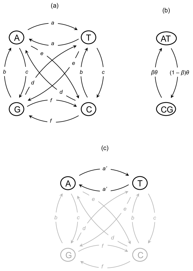
Figure 2: (a) The rate matrix with strand symmetry, Eq. (47), (b) the effective 2-allele rate matrix with alleles grouped as $(AG)$ and $(CG)$, Eq. (54), and (c) the effective rate matrix conditioning on the event that a site is occupied by only $A$ and/or $T$ alleles, Eq. (60).

6.1 Stationary strand-symmetric sampling distribution

The stationary distribution of the rate matrix Eq. (47) is

$$\pi^{\rm T}=\tfrac{1}{2}(\begin{array}[]{cccc}\beta&\beta&1-\beta&1-\beta\end{array}),$$ (48)

where

$$\beta=\frac{b+d}{b+d+c+e}.$$ (49)

Combining Eqs. (47) and (6) gives the stationary sampling distribution to first order in the elements of $\mathbf{Q}$ as

$$\Pr(\mathbf{Y}=\mathbf{y}\mid\mathbf{Q})=$$ (50)

$$\begin{cases}\displaystyle\tfrac{1}{2}\{\beta(1-(a+c+e)H_{M-1})\},&y_{A}=M,\quad y_{T,G,C}=0\\ &\text{or }y_{T}=M,\quad y_{A,G,C}=0;\\ \\ \displaystyle\tfrac{1}{2}\{(1-\beta)(1-(b+d+f)H_{M-1})\},&y_{G}=M,\quad y_{A,T,C}=0;\\ &\text{or }y_{C}=M,\quad y_{A,T,G}=0;\\ \displaystyle\tfrac{1}{2}\beta a\left\{\frac{1}{y_{T}}+\frac{1}{y_{A}}\right\},&y_{T}+y_{A}=M,\,y_{C}=y_{G}=0;\\ \\ \displaystyle\tfrac{1}{2}\left\{\beta\frac{e}{y_{C}}+(1-\beta)\frac{d}{y_{A}}\right\},&y_{C}+y_{A}=M,\,y_{T}=y_{G}=0;\\ \\ \displaystyle\tfrac{1}{2}\left\{\beta\frac{e}{y_{G}}+(1-\beta)\frac{d}{y_{T}}\right\},&y_{G}+y_{T}=M,\,y_{C}=y_{A}=0:\\ \\ \displaystyle\tfrac{1}{2}\left\{\beta\frac{c}{y_{G}}+(1-\beta)\frac{b}{y_{A}}\right\},&y_{G}+y_{A}=M,\,y_{C}=y_{T}=0;\\ \\ \displaystyle\tfrac{1}{2}\left\{\beta\frac{c}{y_{C}}+(1-\beta)\frac{b}{y_{T}}\right\},&y_{C}+y_{T}=M,\,y_{G}=y_{A}=0;\\ \\ \displaystyle\tfrac{1}{2}(1-\beta)f\left\{\frac{1}{y_{G}}+\frac{1}{y_{C}}\right\},&y_{G}+y_{C}=M,\,y_{T}=y_{A}=0;\\ \\ 0,&y_{k},y_{l},y_{m}>0\text{ for distinct}\\ &\text{$k$, $l$, $m$.}\end{cases}$$

In Section 5 we isolated sufficient statistics within site frequency data for estimating certain combinations of parameters of $\mathbf{Q}$ by factoring the likelihood Eq. (12). Here we take a slightly different approach and carry out the factorisation at the level of the sampling distribution. This approach is equivalent in that it ultimately relies on properties of the multinomial distribution behind the likelihood, but is more suited to the strand-symmetric rate matrix. Define the reparametrization

$$\begin{split}\beta&=\frac{b+d}{\theta},\\ \gamma&=\frac{(b+d)(c+e)}{b+d+c+e}=\beta(1-\beta)\theta,\\ a^{\prime}&=\frac{\beta a}{\beta-\gamma H_{M-1}},\\ b^{\prime}&=\frac{b}{b+d},\\ e^{\prime}&=\frac{e}{c+e},\\ f^{\prime}&=\frac{(1-\beta)f}{1-\beta-\gamma H_{M-1}},\end{split}$$ (51)

where

$$\theta=b+c+d+e.$$ (52)

In terms of the six new parameters, the distribution Eq. (50) factorises as

$$\Pr(\mathbf{Y}=\mathbf{y}\mid\mathbf{Q})=$$ (53)

$$\begin{cases}\tfrac{1}{2}(\beta-H_{M-1}\gamma)(1-H_{M-1}a^{\prime}),&(y_{A}=M,y_{T,G,C}=0)\text{ or}\\ &(y_{T}=M,y_{A,G,C}=0);\\ \\ \tfrac{1}{2}((1-\beta)-H_{M-1}\gamma)(1-H_{M-1}f^{\prime}),&(y_{C}=M,y_{A,T,G}=0)\text{ or}\\ &(y_{G}=M,y_{A,T,C}=0);\\ \tfrac{1}{2}\displaystyle(\beta-H_{M-1}\gamma)a^{\prime}\left(\frac{1}{y_{T}}+\frac{1}{y_{A}}\right),&1\leq y_{T},y_{A}\leq M-1,\\ &y_{T}+y_{A}=M;\\ \tfrac{1}{2}\displaystyle\gamma\left(\frac{e^{\prime}}{y}+\frac{1-b^{\prime}}{M-y}\right),&(y_{C}=y,y_{A}=M-y)\text{ or }\\ &(y_{G}=y,y_{T}=M-y);\\ \\ \tfrac{1}{2}\displaystyle\gamma\left(\frac{1-e^{\prime}}{y}+\frac{b^{\prime}}{M-y}\right),&(y_{G}=y,y_{A}=M-y)\text{ or }\\ &(y_{C}=y,y_{T}=M-y);\\ \\ \tfrac{1}{2}\displaystyle(1-\beta-H_{M-1}\gamma)f^{\prime}\left(\frac{1}{y_{G}}+\frac{1}{y_{C}}\right),&1\leq y_{G},y_{C}\leq M-1,\\ &y_{G}+y_{C}=M\,;\\ \\ 0,&y_{k},y_{l},y_{m}>0\text{ for distinct}\\ &\text{$k$, $l$, $m$,}\end{cases}$$

correct to first order in the elements of $\mathbf{Q}$.

The motivation for the choice of $\beta$ and $\gamma$ in Eq.(51) comes from partitioning the genomic alphabet into two effective alleles, $(AT)$ and $(CG)$. Following the procedure described in Appendix B of Burden and Tang [6] the effective 2-allele model corresponds to the $2\times 2$ rate matrix (see Fig. 2(b))

$$\widetilde{\mathbf{Q}}=\left(\begin{array}[]{cc}Q_{(AT),(AT)}&Q_{(AT),(CG)}\\ Q_{(CG),(AT)}&Q_{(CG),(CG)}\end{array}\right)=\theta\left(\begin{array}[]{cc}\beta-1&1-\beta\\ \beta&-\beta\end{array}\right),$$ (54)

whose stationary distribution is

$$\widetilde{\pi}^{\rm T}=\left(\begin{array}[]{cc}\beta&1-\beta\end{array}\right).$$ (55)

Note that the equivalence to a 2-allele model only extends to the stationary distribution as, in general, there is no 2-state Markov chain dynamically equivalent to the partitioning of a given multi-state Markov chain. The stationary sampling distribution of a diffusion-limit 2-allele mutation-drift model is solved in Section 4 of Vogl [26]. Translated to the notation of the current paper, Vogl’s result is

$$\Pr(Y_{A}+Y_{T}=y,Y_{C}+Y_{G}=M-y\mid\mathbf{Q})$$ (56)

$$= \Pr(\widetilde{Y}_{(AT)}=y,\widetilde{Y}_{(CG)}=M-y\mid\widetilde{\mathbf{Q}})$$

$$= \begin{cases}\beta-\gamma H_{M-1}+\mathcal{O}(\theta^{2}),&y=M;\\ \displaystyle\gamma\left(\frac{1}{y}+\frac{1}{M-y}\right)+\mathcal{O}(\theta^{2}),&1\leq y\leq M-1;\\ 1-\beta-\gamma H_{M-1}+\mathcal{O}(\theta^{2}),&y=0.\end{cases}$$

It is straightforward to check that Eq. (56) is indeed the marginal distribution of Eq. (53).

The motivation for the choice of $a^{\prime}$ in Eq. (51) comes from conditioning on the event that the sampled site is occupied by only $A$ or $T$ alleles (see Fig. 2(c)). From Eq, (50) and the definition of $\gamma$, we have

$$\Pr(Y_{A}+Y_{T}=M\mid\mathbf{Q})=\beta(1-(c+e)H_{M-1})=\beta-\gamma H_{M-1}.$$ (57)

The conditional probability that the site is occupied by $y$ $A$-alleles and $(M-y)$ $T$-alleles is then

$$\Pr(Y_{A}=y\mid Y_{A}+Y_{T}=M,\mathbf{Q})$$ (58)

$$= \frac{\Pr(Y_{A}=y,Y_{T}=M-y\mid\mathbf{Q})}{\Pr(Y_{A}+Y_{T}=M,\mid\mathbf{Q})}$$

$$= \begin{cases}\displaystyle\frac{\tfrac{1}{2}\beta(1-(a+c+e)H_{M-1})}{\beta-\gamma H_{M-1}},&y=0\text{ or }y=M;\\ \displaystyle\frac{\tfrac{1}{2}\beta a}{\beta-\gamma H_{M-1}}\left(\frac{1}{y}+\frac{1}{M-y}\right),&y=1,\ldots,M-1\end{cases}$$

$$= \begin{cases}\displaystyle\tfrac{1}{2}\left(1-\frac{\beta a}{\beta-\gamma H_{M-1}}H_{M-1}\right),&y=0\text{ or }y=M;\\ \displaystyle\tfrac{1}{2}\frac{\beta a}{\beta-\gamma H_{M-1}}\left(\frac{1}{y}+\frac{1}{M-y}\right),&y=1,\ldots,M-1.\end{cases}$$

With the definition of $a^{\prime}$ in Eq. (51) this simplifies to

$$\Pr(Y_{A}=y\mid Y_{A}+Y_{T}=M,\mathbf{Q})=\begin{cases}\tfrac{1}{2}(1-a^{\prime}H_{M-1}),&y=0\text{ or }y=M;\\ \tfrac{1}{2}a^{\prime}\displaystyle\left(\frac{1}{y}+\frac{1}{M-y}\right),&y=1,\ldots,M-1.\end{cases}$$ (59)

Comparing with Eq. (56), it is clear this is the sampling distribution for an effective 2-allele mutation-drift model with rate matrix

$$\tilde{\mathbf{Q}}^{(AT)}=a^{\prime}\left(\begin{array}[]{rr}-1&1\\ 1&-1\end{array}\right).$$ (60)

This interpretation is evident in the first and third lines of Eq. (53). An analogous argument holds for the choice of parameter $f^{\prime}$ by conditioning on the event that the sampled site is occupied by only $C$ or $G$ alleles.

6.2 Strand-symmetric parameter estimation

Assume a dataset in the form of a site frequency spectrum obtained by sampling $L$ independent neutrally evolving sites within a multiple alignment of $M$ genomes with allele occupancy counts defined as in Eqs. (8) and (9). Also define

$$\begin{split}L^{(AT)}&=L_{A}+L_{T}+L_{AT}\\ L^{(CG)}&=L_{C}+L_{G}+L_{CG}\\ L^{(AT,CG)}&=L_{AC}+L_{AG}+L_{TC}+L_{TG}.\end{split}$$ (61)

Since Eq. (6) implies that tri-allelic and tetra-allelic sites only occur with probability ${\mathcal{O}}(\theta^{2})$, as in Section 3 assume that

$$L=\sum_{i}L_{i}+L_{\rm P}=L^{(\rm AT)}+L^{(\rm CG)}+L^{(\rm AT,CG)}.$$ (62)

From Eq. (53) we obtain the likelihood function

$${\cal L}(\beta,\gamma,a^{\prime},b^{\prime},e^{\prime}f^{\prime}\mid l_{i},l_{ij}(y))=\Pr\left(L_{i}=l_{i},L_{ij}(y)=l_{ij}(y)\mid\mathbf{Q}\right)$$

$$= \frac{L!}{(\prod_{i}l_{i}!)(\prod_{i<j}\prod_{y=1}^{M-1}l_{ij}(y)!)}\times\left\{\tfrac{1}{2}(\beta-H_{M-1}\gamma)(1-H_{M-1}a^{\prime})\right\}^{l_{A}+l_{T}}$$

$$\qquad\times\left\{\tfrac{1}{2}(1-\beta-H_{M-1}\gamma)(1-H_{M-1}f^{\prime})\right\}^{l_{C}+l_{G}}$$

$$\qquad\times\left\{\tfrac{1}{2}(\beta-H_{M-1}\gamma)a^{\prime}\right\}^{L_{AT}}\prod_{y=1}^{M-1}\left(\frac{1}{M-y}+\frac{1}{y}\right)^{l_{AT}(y)}$$

$$\qquad\times\left\{\tfrac{1}{2}(1-\beta-H_{M-1}\gamma)f^{\prime}\right\}^{L_{CG}}\prod_{y=1}^{M-1}\left(\frac{1}{M-y}+\frac{1}{y}\right)^{l_{CG}(y)}$$

$$\qquad\times\left(\tfrac{1}{2}\gamma\right)^{L_{AC}+L_{TG}}\prod_{y=1}^{M-1}\left(\frac{e^{\prime}}{M-y}+\frac{1-b^{\prime}}{y}\right)^{l_{AC}(y)+l_{TG}(y)}$$

$$\qquad\times\left(\tfrac{1}{2}\gamma\right)^{L_{AG}+L_{TC}}\prod_{y=1}^{M-1}\left(\frac{1-e^{\prime}}{M-y}+\frac{b^{\prime}}{y}\right)^{l_{AG}(y)+l_{TC}(y)}$$

$$= \text{(const.)}\times(2H_{M-1}\gamma)^{l^{(AT,CG)}}$$

$$\qquad\times\left\{(1-H_{M-1}\gamma)H_{M-1}a^{\prime}\right\}^{l_{AT}}$$

$$\qquad\times\left\{(1-H_{M-1}\gamma)(1-H_{M-1}a^{\prime})\right\}^{l_{A}+L_{T}}$$

$$\qquad\times\left\{(1-\beta-H_{M-1}\gamma)H_{M-1}f^{\prime}\right\}^{l_{CG}}$$

$$\qquad\times\left\{(1-\beta-H_{M-1}\gamma)(1-H_{M-1}f^{\prime})\right\}^{l_{C}+l_{G}}$$

$$\qquad\times\prod_{y=1}^{M-1}\left\{\left(\frac{e^{\prime}}{M-y}+\frac{1-b^{\prime}}{y}\right)^{l_{AC}(y)+l_{TG}(y)}\left(\frac{1-e^{\prime}}{M-y}+\frac{b^{\prime}}{y}\right)^{l_{AG}(y)+l_{TC}(y)}\right\},$$

where the constant is a combinatorial factor independent of $\beta$, $\gamma$, $a^{\prime}$, $b^{\prime}$, $e^{\prime}$, and $f^{\prime}$. This is a multinomial distribution, which can be factored in two different ways.

Firstly, recall the notation $\vec{l}_{ij}$ defined by Eq. (40) and consider

$${\cal L}(\beta,\gamma,a^{\prime},b^{\prime},e^{\prime}f^{\prime}\mid l_{i},l_{ij}(y))=g(l^{(AT)},l^{(CG)},l^{(AT,CG)};\beta,\gamma)$$ (64)

$$\qquad\times h(l_{A},l_{T},l_{C},l_{G},l_{AT},l_{CG},\vec{l}_{AC},\vec{l}_{TG},\vec{l}_{AG},\vec{l}_{TC};a^{\prime},f^{\prime},b^{\prime}e^{\prime}),$$

where

$$g(l^{(AT)},l^{(CG)},l^{(AT,CG)};\beta,\gamma)=\frac{L!}{l^{(AT)})!l^{(CG)}!l^{(AT,CG)}!}$$ (65)

$$\quad\times(\beta-H_{M-1}\gamma)^{l^{(AT)}}(1-\beta-H_{M-1}\gamma)^{l^{(CG)}}(2H_{M-1}\gamma)^{l^{(AT,CG)}},$$

and the function $h(\cdot)$ is a product of the remaining factors times an appropriate combinatorial factor to ensure that $\cal L$ is correctly normalised. Following the same procedure as for the general rate matrix, observe that $h(\cdot)$ is independent of $\beta$ and $\gamma$, and that Neyman factorisation then implies that $L^{(AT)}$, $L^{(CG)}$ and $L^{(AT,CG)}$ are sufficient statistics for estimating $\beta$ and $\gamma$. Summing over the redundant allele occupancy counts subject to conditioning on $L^{(AT)}=l^{(AT)}$, $L^{(CG)}=l^{(CG)}$ and $L^{(AT,CG)}=l^{(AT,CG)}$ gives the flat family of trinomials $g(l^{(AT)},l^{(CG)},l^{(AT,CG)};\beta,\gamma)$, from which we read off the minimum variance, unbiased, ML estimators

$$\widehat{\beta-H_{M-1}\gamma}=\frac{L^{(AT)}}{L},\qquad\widehat{2H_{M-1}\gamma}=\frac{L^{(AT,CG)}}{L}.$$ (66)

By linearity we therefore have that

$$\hat{\beta}=\frac{L^{(AT)}+\tfrac{1}{2}L^{(AT,CG)}}{L},\qquad\hat{\gamma}=\frac{L^{(AT,CG)}}{2LH_{M-1}},$$ (67)

are unbiased ML estimators. These estimators agree precisely with corresponding estimators derived by Vogl [26, Section 4.1] and re-derived in Section 5.1 for the 2-allele mutation-drift model with stationary sampling distribution equivalent to Eq. (56).

Secondly, consider the factorisation

$${\cal L}(\beta,\gamma,a^{\prime},b^{\prime},e^{\prime}f^{\prime}\mid l_{i},l_{ij}(y))$$ (68)

$$= g(l_{A}+l_{T},l_{C}+l_{G},l_{AT},l_{CG},l^{(AT,CG)};\beta,\gamma,a^{\prime},f^{\prime})$$

$$\qquad\times h(\vec{l}_{AC},\vec{l}_{TG},\vec{l}_{AG},\vec{l}_{TC};b^{\prime}e^{\prime}),$$

where

$$g(l_{A}+l_{T},l_{C}+l_{G},l_{AT},l_{CG},l^{(AT,CG)};\beta,\gamma,a^{\prime},f^{\prime})$$ (69)

$$= \frac{L!}{l^{(AT,CG)}!l_{AT}!(l_{A}+l_{T})!l_{CG}!(l_{C}+l_{G})!}$$

$$\times(2H_{M-1}\gamma)^{l^{(AT,CG)}}{p_{AT}}^{l_{AT}}{p_{A+T}}^{l_{A}+l_{T}}{p_{CG}}^{l_{CG}}{p_{C+G}}^{l_{C}+l_{G}},$$

with

$$\begin{split}p_{AT}&=(\beta-H_{M-1}\gamma)H_{M-1}a^{\prime}=H_{M-1}\beta a\\ p_{A+T}&=(\beta-H_{M-1}\gamma)(1-H_{M-1}a^{\prime})\\ p_{CG}&=(1-\beta-H_{M-1}\gamma)H_{M-1}f^{\prime}=H_{M-1}(1-\beta)f\\ p_{C+G}&=(1-\beta-H_{M-1}\gamma)(1-H_{M-1}f^{\prime})\\ \end{split}$$ (70)

and $h(\vec{l}_{AC},\vec{l}_{TG},\vec{l}_{AG},\vec{l}_{TC};b^{\prime}e^{\prime})$ is the final product in Eq. (6.2) times an appropriate combinatorial factor to ensure that $\cal L$ is correctly normalised. Applying Neyman factorisation as before to factor out $h(.)$, and recognising Eq. (69) as a flat family of fifth order multinomials in 4 independent parameters, we obtain the minimum variance, unbiased, ML estimators $\hat{p}_{AT}=L_{AT}/L$ and $\hat{p}_{CG}=L_{CG}/L$. Thus

$$\begin{split}\widehat{\beta a}=\frac{L_{AT}}{LH_{M-1}},\\ \widehat{(1-\beta)f}=\frac{L_{CG}}{LH_{M-1}},\end{split}$$ (71)

are minimum variance, unbiased ML estimators.

There is no simple analytic formula for the ML estimators $\widehat{b^{\prime}}$ and $\widehat{e^{\prime}}$. However they can be easily computed by maximising the conditional log-likelihood arising from $h(\vec{l}_{AC},\vec{l}_{TG},\vec{l}_{AG},\vec{l}_{TC};b^{\prime}e^{\prime})$, namely

$$\log{\cal L}(e^{\prime},b^{\prime}) = \sum_{y=1}^{M-1}\left\{(l_{AC}(y)+l_{TG}(y))\log\left(\frac{e^{\prime}}{M-y}+\frac{1-b^{\prime}}{y}\right)\right.$$ (72)

$$\quad\left.+\,(l_{AG}(y)+l_{TC}(y))\log\left(\frac{1-e^{\prime}}{M-y}+\frac{b^{\prime}}{y}\right)\right\}$$

over the region $(b^{\prime},e^{\prime})\in[0,1]\times[0,1]$. This can be done using, for instance, the R function constrOptim( ) or the EM algorithm described in A. The maximum is unique by the following argument: Set $\ell_{1}(y)=l_{AC}(y)+l_{TG}(y)$, $\ell_{2}(y)=l_{AG}(y)+l_{TC}(y)$ and

$$G_{1}(y)=\frac{e^{\prime}}{M-y}+\frac{1-b^{\prime}}{y},\qquad G_{2}(y)=\frac{1-e^{\prime}}{M-y}+\frac{b^{\prime}}{y}.$$

Assuming $\min_{y}(\ell_{1}(y),\ell_{2}(y))>0$, the Hessian matrix

$${\cal H} = \left(\begin{array}[]{cc}\dfrac{\partial^{2}\log{\cal L}}{\partial e^{\prime 2}}&\dfrac{\partial^{2}\log{\cal L}}{\partial e^{\prime}\partial b^{\prime}}\\ \\ \dfrac{\partial^{2}\log{\cal L}}{\partial e^{\prime}\partial b^{\prime}}&\dfrac{\partial^{2}\log{\cal L}}{\partial b^{\prime 2}}\end{array}\right)$$ (76)

$$= \sum_{y=1}^{M-1}\left(\frac{\ell_{1}}{G_{1}^{2}}+\frac{\ell_{2}}{G_{2}^{2}}\right)\left(\begin{array}[]{cc}\dfrac{-1}{(M-y)^{2}}&\dfrac{1}{y(M-y)}\\ \\ \dfrac{1}{y(M-y)}&\dfrac{-1}{y^{2}}\end{array}\right),$$ (80)

is negative definite since for any real $\mathbf{u}^{\rm T}=(u_{1},u_{2})$,

$$\mathbf{u}^{\rm T}{\cal H}\mathbf{u}=-\sum_{y=1}^{M-1}\left(\frac{\ell_{1}(y)}{G_{1}(y)^{2}}+\frac{\ell_{2}(y)}{G_{2}(y)^{2}}\right)\left(\frac{u_{1}}{M-y}-\frac{u_{2}}{y}\right)^{2}<0.$$ (81)

Therefore any stationary point in the connected region for which $\log{\cal L}(e^{\prime},b^{\prime})$ is real must be an isolated local maximum. More than one maximum cannot occur without there being a saddle point on a curve connecting them, so the maximum is unique.

To obtain ML estimators of the strand-symmetric Q parameters $(a,\ldots,e)$ in Eq. (47), we invert Eq. (51) to give

$$\begin{split}b&=b^{\prime}\frac{\gamma}{1-\beta},\\ c&=(1-e^{\prime})\frac{\gamma}{\beta},\\ d&=(1-b^{\prime})\frac{\gamma}{1-\beta},\\ e&=e^{\prime}\frac{\gamma}{\beta},\\ \end{split}$$ (82)

Then from Eqs. (67), (71) and (82) we obtain the ML estimators

$$\begin{split}\hat{a}&=\frac{1}{H_{M-1}}\frac{L_{AT}}{L^{(AT)}+\tfrac{1}{2}L^{(AT,CG)}},\\ \hat{b}&=\frac{\widehat{b^{\prime}}}{2H_{M-1}}\frac{L^{(AT,CG)}}{L^{(CG)}+\tfrac{1}{2}L^{(AT,CG)}},\\ \hat{c}&=\frac{1-\widehat{e^{\prime}}}{2H_{M-1}}\frac{L^{(AT,CG)}}{L^{(AT)}+\tfrac{1}{2}L^{(AT,CG)}},\\ \hat{d}&=\frac{1-\widehat{b^{\prime}}}{2H_{M-1}}\frac{L^{(AT,CG)}}{L^{(CG)}+\tfrac{1}{2}L^{(AT,CG)}},\\ \hat{e}&=\frac{\widehat{e^{\prime}}}{2H_{M-1}}\frac{L^{(AT,CG)}}{L^{(AT)}+\tfrac{1}{2}L^{(AT,CG)}},\\ \hat{f}&=\frac{1}{H_{M-1}}\frac{L_{CG}}{L^{(CG)}+\tfrac{1}{2}L^{(AT,CG)}}.\end{split}$$ (83)

Note that these estimators are in general biased.

7 Application

Bergman et al. [3] extracted sequence information of 197 Drosophila melanogaster individuals [15] on the short autosomal introns (i.e. the nucleotides in positions $8$ through $30$ of introns $\leq 65$ bp in length), resulting in a site frequency spectrum of 218,942 nucleotides. This dataset is one of the largest and most accurate available today. As the population of D. melanogaster does not seem to be in equilibrium but instead exhibits a bias towards $C$ and $G$ nucleotides, the data are nevertheless not ideal for our purpose.

We implemented our ML estimators in the statistical programming language R [18]. The ML estimate of the general rate matrix $\mathbf{Q}$ was determined using Eqs. (39) to estimate $\pi_{1}^{\prime}$, $\pi_{2}^{\prime}$, $\pi_{3}^{\prime}$ and $C$, and the R function constrOptim() to maximise $h(\bm{\ell}_{\rm P};c_{ij},\phi_{ij})$ defined by Eq. (5.2) with respect to the set of independent parameters $c_{ij}$ and $\phi_{ij}$ defined in Eq. (30). For $K=4$ this amounts to five $c_{ij}$’s and three $\phi_{ij}$’s, i.e. a total of eight parameters to be determined numerically. To optimise performance of the program a rough approximation to the maximum likelihood estimates of $c_{ij}$ and $\phi_{ij}$ is first determined from the simpler but incorrect method in Burden and Tang [7, p 28], and this approximation is then used as a starting values in the function constrOptim() for the full 8 parameter optimizaton. With this strategy the maximum likelihood estimate for the full 12-parameter model was calculated correct to 5 significant figures in less than 1 second on a MacBook Air laptop computer with a 1.8 GHz Intel Core i5 processor. The estimate of the rate matrix reconstructed via Eqs. (18) and (29) is

$$\hat{\mathbf{Q}}=\left(\begin{array}[]{rrrr}-0.018072&0.006464&0.007479&0.004129\\ 0.006215&-0.017885&0.003640&0.008030\\ 0.016583&0.007047&-0.028496&0.004866\\ 0.006590&0.015678&0.004466&-0.026734\end{array}\right),$$ (84)

where rows and columns are ordered $(A,T,G,C)$.

Similarly the ML estimator assuming reversibility was calculated from Eqs. (18) and (46) with $\hat{\Phi}_{ij}\equiv 0$ as

$$\hat{\mathbf{Q}}^{\text{rev}}=\left(\begin{array}[]{rrrr}-0.018077&0.006452&0.007697&0.003928\\ 0.006227&-0.017882&0.003483&0.008173\\ 0.015987&0.007495&-0.028477&0.004996\\ 0.007098&0.015302&0.004346&-0.026747\end{array}\right).$$ (85)

The ML estimator assuming strand symmetry was calculated from Eqs. (47) and (83), with $\widehat{b^{\prime}}$ and $\widehat{e^{\prime}}$ obtained by numerically maximising Eq. (72), to obtain

$$\hat{\mathbf{Q}}^{\text{strand-sym}}=\left(\begin{array}[]{rrrr}-0.017978&0.006337&0.007760&0.003880\\ 0.006337&-0.017978&0.003880&0.007760\\ 0.016099&0.006804&-0.027552&0.004649\\ 0.006804&0.016099&0.004649&-0.027552\end{array}\right).$$ (86)

Although the three estimated rate matrices do not differ greatly, the differences enable us to quantify the significance of the deviation of the general model from reversibility and strand symmetry. If reversibility (resp. strand symmetry) is taken as a null hypothesis and the general rate matrix taken as the alternate hypothesis, the log of the likelihood ratio statistic,

$$-2\left[\log{\cal L}(\hat{\mathbf{Q}}^{\text{null}}\mid\bm{\ell})-\log{\cal L}(\hat{\mathbf{Q}}^{\text{alt}}\mid\bm{\ell})\right],$$ (87)

will asymptotically (as the number of sites $L\rightarrow\infty$) have a chi-squared distribution with $d=3$ (resp. $d=6$) degrees of freedom if the extra parameters required to specify the general rate matrix are not significant. Setting $\hat{\mathbf{Q}}^{\text{null}}=\hat{\mathbf{Q}}^{\text{rev}}$ or $\hat{\mathbf{Q}}^{\text{strand-sym}}$ in Eqs. (12) and (87) gives p-values of $3.6\times 10^{-5}$ and $<10^{-91}$ respectively, indicating significant deviations from both reversibility and strand symmetry for this dataset. Note that Bergman et al. [3] report slight but significant deviations from Chargaff’s second parity rule.

In all three models, estimates for scaled mutation rates are higher for transitions ($A\leftrightarrow G$ and $C\leftrightarrow T$) than for transversions (($A\text{ or }G)\leftrightarrow(C\text{ or }T$)), as expected. By considering a sample of size $M=2$ in the sampling distribution Eq. (6), the first order approximation to the expected heterozygosity is

$$1-\sum_{i}\hat{\pi}_{i}\left(1-\sum_{j\neq i}\hat{Q}_{ij}\right)=-\sum_{i\in\{A,T,G,C\}}\hat{\pi}_{i}\hat{Q}_{ii}.$$ (88)

For all three models this gives an identical expected heterozygosity of 0.0212.

8 Simulation

To assess the accuracy of the small-$\theta$ approximation we have simulated datasets of site frequency spectra corresponding to sampling of $M$ individuals from a finite population of size $N$ at $L$ independent genomic sites. For a given rate matrix $Q$ we begin by numerically determining the stationary distribution of the finite population Wright-Fisher model with neutral mutation rates $u_{ij}=(\exp(Q/(2N)))_{ij}$, consistent with Eq. (1). For this step the full ${N+K-1\choose K-1}\times{N+K-1\choose K-1}$ Markov transition matrix is used, where $K=4$ for the genomic alphabet $\{A,T,G,C\}$. For each site within each dataset, the allele occupancies are determined by drawing from a multinomial distribution corresponding to $M$ trials from $K$ categories with probabilities of success in each category determined by a random draw from the Wright-Fisher stationary distribution. For each dataset this leads to site frequency data as defined by Eq. (8) from which an estimate $\hat{Q}$ of the full rate matrix is obtained from Eqs. (5.2) and (39) as described in Section 5.2.

In order to illustrate the limit of applicability of the small-$\theta$ approximation we consider two examples for the ‘true’ rate matrix $Q$: (i) the matrix given by Eq. (84) obtained from the Drosophila melanogaster of the previous section, and (ii) the same matrix multiplied by $0.1$. The population size, which is constrained by the computational demands of determining the stationary state of a large Markov transition matrix, is chosen to be $N=40$. Note that in general the diffusion $N\to\infty$ limit is approached very rapidly for the stationary distribution of a neutral Wright-Fisher model (see for example Burden and Tang [6, Figs. 5 and 6].) We have aimed to satisfy the ideal limit $1<<M<<N$ within the constraints of the simulation by choosing the sample size $M=10$. The number of genomic sites is $L=10^{5}$.

Figures 3 and 4 show histograms of the estimated rate matrix elements from $1000$ simulated datasets, together with the ‘true’ matrix elements for the two rate matrices. The off-diagonal elements of $Q$ are generally underestimated in Fig. 3 and, given that the diagonal elements are simply calculated as minus the sum of estimates of the off-diagonal row elements, the diagonal elements are correspondingly overestimated. By comparison, the off-diagonal elements in Fig. (4) are slightly underestimated, but generally acceptable. The sum of the off-diagonal elements is $0.0912$ for the rate matrix in Fig. 3 and $0.00912$ for the rate matrix in Fig. 4. We conclude that, as a rule of thumb, the small-$\theta$ approximation will provide acceptable estimates provided the sum of the off-diagonal elements of the scaled rate matrix is less than $10^{-2}$. Note that the widths of the histograms are determined by the sample size $M$, which is necessarily small in this simulation due to computational constraints, and are not indicative of standard errors expected in a biological dataset such as the Drosophila melanogaster dataset used in the previous section.

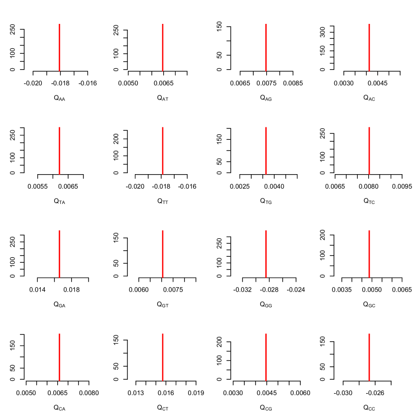
Figure 3: Histograms of estimates $\hat{Q}_{ij}$ of the rate matrix obtained from $1000$ synthetic datasets corresponding to sampling $M=10$ individuals from a stationary-distribution population of $N=40$ neutrally evolving haploid individuals at $L=10^{5}$ genomic sites. Elements of ‘true’ rate matrix, Eq. (84), are shown as red vertical bars.

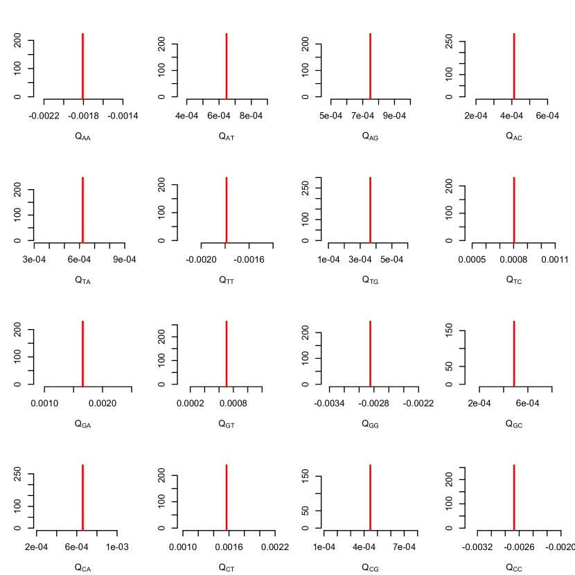
Figure 4: Same as Fig. 3, except that the ‘true’ rate matrix is chosen to be $0.1$ times the matrix in Eq. (84).

9 Conclusions

We have obtained ML estimates of a scaled rate matrix from population allele frequencies observed in unlinked neutrally evolving, independent genomic sites under three sets of model assumptions: that the rate matrix is unconstrained, that it is reversible, and that it is strand-symmetric. The analysis is carried out to first order in scaled mutation rates $Q_{ij}$ defined by Eq. (1), which are assumed to be small. This is equivalent to assuming that at most one mutation has occurred in the coalescent tree of the example, and hence that the sample includes only non-segregating and bi-allelic sites. The purpose of our analysis is twofold:

Firstly, our treatment is more rigorous than a previous analysis of this problem by Burden and Tang [7, p28], and corrects an error in that earlier analysis. The correct estimates, specifically for the case of a general unconstrained rate matrix and for the assumption of a strand-symmetric rate matrix, are given in Sections 5.2 and 6.2 respectively of the current paper. Although the correction is generally small in absolute terms, it is necessary for an accurate significance test of violation of reversibility and strand symmetry via the likelihood ratio statistic Eq. (87).

Secondly, in Section 7 we have demonstrated efficient software in R implementing ML estimates for a biological dataset consisting of a site frequency spectrum extracted from short autosomal introns in a sample of Drosophila melanogaster individuals. This software is available at the web address given below, and requires as input a table of allele occupancy counts as defined by Eq. (8).

It is worth stressing the limits on the use of our software for rate matrix estimation: The theory leading to the likelihood function Eq. (12) assumes a mutation-drift model corresponding to the backward generator Eq. (2), that is, the diffusion limit of a Moran or Wright-Fisher model for a population of constant size. Substitutions are assumed to be due to neutral mutations with no directional selection. Although Vogl and Bergman [27] have performed a similar ML analysis for the analogous bi-allelic model with selection parameters, we are unaware of any analytic solution for the multi-allelic sampling distribution with selection.

The likelihood function is derived from the stationary sampling distribution. As pointed out in Section 7 the assumption of stationarity may not hold for our test Drosophila melanogaster dataset. The non-stationary sampling distribution has been derived to first order in $Q_{ij}$ by Burden and Griffiths [5], and is considerably more complicated than the stationary distribution, Eq. (6). Nevertheless it has the potential to serve as a basis for estimating neutral mutation rates in a non-stationary setting.

The theory also assumes that the genomic loci should not only be neutrally evolving, but should have independent ancestries to avoid correlations due to common coalescent trees [22]. This should be possible in randomly mating diploid populations by choosing loci which are unlinked due to recombination. There is strong evidence that this requirement is satisfied for the Drosophila melanogaster dataset analysed in Section 7 [8].

Finally, we stress that the first order analysis we have used assumes that all off-diagonal elements of $\mathbf{Q}$ are small. For situations where this is not the case it is necessary to resort to other approximation methods such as importance sampling [24], which, as noted by De Iorio and Griffiths [9, p421–2], are only expected to be exact for a parent-independent rate matrix, in which case the sampling distribution is known to be multinomial-Dirichlet. Application of importance sampling to the related problem of a mutations in a subdivided population with high mutation and migration rates have unfortunately proved to be considerably more computationally intensive than computations in the current paper [10].

Numerical simulations in Section 8 indicate that the small $\theta$ approximation will provide acceptable results provided the sum of the off-diagonal elements of $\mathbf{Q}$ are less than $10^{-2}$. While the Drosophila melanogaster short intron dataset used in Section 7 appears to be just beyond the limit of of this restriction, the condition is believed to be satisfied in general for silent sites in protein coding genes in eukaryote genomes [17].

Software

The R programs developed for estimating rate matrices, testing accuracy of the likelihood maximisation, significance testing, and calculating heterozygosity in Sections 7 and 8 are available at https://github.com/cjb105/RateMatrixEstimation.

Appendix A Appendix, Expectation-Maximisation Algorithm algorithm

Here we provide the expectation-maximisation (EM) algorithm that can be used to estimate $e^{\prime}$ and $b^{\prime}$ from the conditional log-likelihood in Eq. (72). Let the unknown auxiliary variable $z_{AC}(y)$ count the number of mutations from $A$ to $C$, the variable $z_{TG}(y)$ those from $T$ to $G$, and similarly for $z_{GA}(y)$ and $z_{CT}(y)$. As a logical consequence, $L_{AC}(y)+L_{TG}(y)-z_{AC}(y)-z_{TG}(y)$ counts the number of mutations from $C$ to $A$ and from $G$ to $T$. Then the conditional log-likelihood can be written as:

$$\begin{split}&\log(\Pr(L_{AC}(y),L_{TG}(y),L_{GA}(y),L_{TC}(y),z_{AC}(y),z_{TG}(y),z_{GA}(y),z_{TC}(y)\mid M,e^{\prime},b^{\prime})=\\ &\qquad const+\sum_{y=1}^{M-1}(z_{AC}(y)+z_{TG}(y))\log\bigg{(}\frac{e^{\prime}}{y}\bigg{)}\\ &\qquad+\sum_{y=1}^{M-1}(L_{AC}(y)+L_{TG}(y)-z_{AC}(y)-z_{TG}(y))\log\bigg{(}\frac{1-b^{\prime}}{M-y}\bigg{)}\\ &\qquad+\sum_{y=1}^{M-1}(z_{GA}(y)+z_{CT}(y))\log\bigg{(}\frac{b^{\prime}}{y}\bigg{)}\\ &\qquad+\sum_{y=1}^{M-1}(L_{GA}(y)+L_{CT}(y)-z_{GA}(y)-z_{CT}(y))\log\bigg{(}\frac{1-e^{\prime}}{M-y}\bigg{)}\,.\end{split}$$ (89)

The expectation step of the EM algorithm constitutes taking the expectation of Eq.( LABEL:eq:cond_ll_em).

It is helpful to look at the conditional expected values of the groups of auxiliary variables $z_{AC}(y)+z_{TG}(y)$, $L_{AC}(y)+L_{TG}(y)-z_{AC}(y)-z_{TG}(y)$, $z_{CA}(y)+z_{GT}(y)$, and $L_{GA}(y)+L_{CT}(y)-z_{GA}(y)-z_{CT}(y)$ separately:

The expectation of $z_{AC}(y)+z_{TG}(y)$ given $L_{AC}(y)+L_{TG}(y)$ corresponds to the mean of a binomial distribution with sample size $L_{AC}(y)+L_{TG}(y)$ and probability $p(y)=\frac{\frac{e^{\prime}}{y}}{\frac{e^{\prime}}{y}+\frac{1-b^{\prime}}{M-y}}$:

$$\operatorname{E}(z_{AC}(y)+z_{TG}(y)\mid L_{AC}(y)+L_{TG}(y))=(L_{AC}(y)+L_{TG}(y))\frac{\frac{e^{\prime t}}{y}}{\frac{e^{\prime t}}{y}+\frac{1-b^{\prime t}}{M-y}}\,.$$ (90)

The other expectations follow analogously.

These can be plugged into Eq. (LABEL:eq:cond_ll_em) to give:

$$\begin{split}&\operatorname{Q}(b^{\prime},e^{\prime}\mid b^{\prime t},e^{\prime t})=\\ &\qquad+\sum_{y=1}^{M-1}(L_{AC}(y)+L_{TG}(y))\frac{\frac{e^{\prime t}}{y}}{\frac{e^{\prime t}}{y}+\frac{1-b^{\prime t}}{M-y}}\log(e^{\prime})\\ &\qquad+\sum_{y=1}^{M-1}(L_{AC}(M-y)+L_{TG}(M-y))\frac{\frac{1-b^{\prime t}}{M-y}}{\frac{e^{\prime t}}{y}+\frac{1-b^{\prime t}}{M-y}}\log(1-b^{\prime})\\ &\qquad+\sum_{y=1}^{M-1}(L_{GA}(y)+L_{CT}(y))\frac{\frac{1-b^{\prime t}}{M-y}}{\frac{1-b^{\prime t}}{y}+\frac{e^{\prime t}}{M-y}}\log(b^{\prime})\\ &\qquad+\sum_{y=1}^{M-1}(L_{GA}(M-y)+L_{CT}(M-y))\frac{\frac{e^{\prime t}}{M-y}}{\frac{1-b^{\prime t}}{y}+\frac{e^{\prime t}}{M-y}}\log(1-e^{\prime})\,.\end{split}$$ (91)

This leaves the maximisation step: To determine the overall iteration scheme for the parameter updates we solve the appropriate derivatives of $\operatorname{Q}(b^{\prime},e^{\prime}\mid b^{\prime t},e^{\prime t})$. The overall iteration scheme is then given by:

$$\begin{split}\hat{e}^{\prime t+1}&=\frac{\sum_{y=1}^{M-1}(L_{AC}(y)+L_{TG}(y))\frac{\frac{e^{\prime t}}{y}}{\frac{e^{\prime t}}{y}+\frac{1-b^{\prime t}}{M-y}}}{\sum_{y=1}^{M-1}(L_{AC}(y)+L_{TG}(y))\frac{\frac{e^{\prime t}}{M-y}}{\frac{e^{\prime t}}{y}+\frac{1-b^{\prime t}}{M-y}}+\sum_{y=1}^{M-1}(L_{GA}(M-y)+L_{CT}(M-y))\frac{\frac{1-e^{\prime t}}{y}}{\frac{1-e^{\prime t}}{y}+\frac{b^{\prime t}}{M-y}}}\\ \hat{b}^{\prime t+1}&=\frac{\sum_{y=1}^{M-1}(L_{GA}(y)+L_{CT}(y))\frac{\frac{b^{\prime t}}{y}}{\frac{b^{\prime t}}{y}+\frac{1-e^{\prime t}}{M-y}}}{\sum_{y=1}^{M-1}(L_{GA}(y)+L_{CT}(y))\frac{\frac{b^{\prime t}}{y}}{\frac{b^{\prime t}}{y}+\frac{1-e^{\prime t}}{M-y}}+\sum_{y=1}^{M-1}(L_{AC}(M-y)+L_{TG}(M-y))\frac{\frac{1-b^{\prime t}}{M-i}}{\frac{e^{\prime t}}{y}+\frac{1-b^{\prime t}}{M-y}}}\,.\end{split}$$ (92)

Cyclical calculation of estimators guarantees convergence towards a local maximum by properties of the EM algorithm. In this case, the local maximum is also the global maximum by the argument in the main text.

References

References

- Baake and Bialowons [2008] Baake, E., Bialowons, R., 2008. Ancestral processes with selection: Branching and Moran models. Stochastic Models in Biological Sciences 80, 33–52.
- Baisnée et al. [2002] Baisnée, P.-F., Hampson, S., Baldi, P., 2002. Why are complementary DNA strands symmetric? Bioinformatics 18 (8), 1021–1033.
- Bergman et al. [2018] Bergman, J., Betancourt, A., Vogl, C., 2018. Transcription-associated compositional skews in drosophila genes. Genome Biology and Evolution 10, 269–275.
- Burden and Griffiths [2019a] Burden, C., Griffiths, R., 2019a. The stationary distribution of a sample from the Wright-Fisher diffusion model with general small mutation rates. Journal of Mathematical Biology 78, 1211–1224.
- Burden and Griffiths [2019b] Burden, C., Griffiths, R., 2019b. The transition distribution of a sample from a Wright–Fisher diffusion with general small mutation rates. Journal of Mathematical Biology 79, 2315–2342.
- Burden and Tang [2016] Burden, C., Tang, Y., 2016. An approximate stationary solution for multi-allele neutral diffusion with low mutation rates. Theoretical Population Biology 112, 22–32.
- Burden and Tang [2017] Burden, C., Tang, Y., 2017. Rate matrix estimation from site frequency data. Theoretical Population Biology 113, 23–33.
- Clemente and Vogl [2012] Clemente, F., Vogl, C., 2012. Unconstrained evolution in short introns? – an analysis of genome-wide polymorphism and divergence data from drosophila. Journal of Evolutionary Biology 25, 1975–1990.
- De Iorio and Griffiths [2004] De Iorio, M., Griffiths, R. C., 2004. Importance sampling on coalescent histories. i. Advances in Applied Probability 36 (2), 417–433.
- De Iorio et al. [2005] De Iorio, M., Griffiths, R. C., Leblois, R., Rousset, F., 2005. Stepwise mutation likelihood computation by sequential importance sampling in subdivided population models. Theoretical population biology 68 (1), 41–53.
- Etheridge [2012] Etheridge, A., 2012. Some Mathematical Models from Population Genetics: Lecture Notes in Mathematics. Springer Verlag. Berlin, Heidelberg.
- Etheridge and Griffiths [2009] Etheridge, A., Griffiths, R., 2009. A coalescent dual process in a Moran model with genic selection. Theoretical Population Biology 75, 320–330.
- Hogg and Craig [1995] Hogg, R. V., Craig, A. T., 1995. Introduction to mathematical statistics. Prentice Hall.
- Keener [2010] Keener, R. W., 2010. Theoretical statistics: Topics for a core course. Springer Texts in Statistics. Springer.
- Lack et al. [2015] Lack, J., Cardeno, C., Crepeau, M., Taylor, W., Corbett-Detig, R., Stevens, K., CH, L., Pool, J., 2015. The drosophila genome nexus: a population genomic resource of 623 drosophila melanogaster genomes, including 197 from a single ancestral range population. Genetics 199(4), 79–87.
- Lobry [1995] Lobry, J., 1995. Properties of a general model of DNA evolution under no-strand-bias conditions. Journal of Molecular Evolution 40, 326–330.
- Lynch et al. [2016] Lynch, M., Ackerman, M., Gout, J., Long, H., Sung, W., Thomas, W., Foster, P., 2016. Genetic drift, selection and the evolution of the mutation rate. Nature 17, 704–714.
-
R Core Team [2017]
R Core Team, 2017. R: A Language and Environment for Statistical Computing. R
Foundation for Statistical Computing, Vienna, Austria.
URL https://www.R-project.org/ - Rosenberg and Nordborg [2002] Rosenberg, N. A., Nordborg, M., 2002. Genealogical trees, coalescent theory and the analysis of genetic polymorphisms. Nature reviews genetics 3 (5), 380.
- RoyChoudhury and Wakeley [2010] RoyChoudhury, A., Wakeley, J., 2010. Sufficiency of the number of segregating sites in the limit under finite-sites mutation. Theoretical Population Biology 78, 118–122.
- Schrempf and Hobolth [2017] Schrempf, D., Hobolth, A., 2017. An alternative derivation of the stationary distribution of the multivariate neutral Wright-Fisher model for low mutation rates with a view to mutation rate estimation from site frequency data. Theoretical Population Biology 114, 88–94.
- Slatkin and Hudson [1991] Slatkin, M., Hudson, R. R., 1991. Pairwise comparisons of mitochondrial DNA sequences in stable and exponentially growing populations. Genetics 129, 555–62.
- Speed et al. [2019] Speed, M. S., Balding, D. J., Hobolth, A., 2019. A general framework for moment-based analysis of genetic data. Journal of Mathematical Biology 78 (6), 1727–1769.
- Stephens and Donnelly [2000] Stephens, M., Donnelly, P., 2000. Inference in molecular population genetics. Journal of the Royal Statistical Society, Series B, Discussion Paper.
- Tataru et al. [2017] Tataru, P., Simonsen, M., Bataillon, T., Hobolth, A., 2017. Statistical inference in the Wright–Fisher model using allele frequency data. Systematic biology 66 (1), e30–e46.
- Vogl [2014] Vogl, C., 2014. Estimating the scaled mutation rate and mutation bias with site frequency data. Theoretical Population Biology 98, 19–27.
- Vogl and Bergman [2015] Vogl, C., Bergman, J., 2015. Inference of directional selection and mutation parameters assuming equilibrium. Theoretical Population Biology 106, 71–82.
- Vogl and Clemente [2012] Vogl, C., Clemente, F., 2012. The allele-frequency spectrum in a decoupled Moran model with mutation, drift, and directional selection, assuming small mutation rates. Theoretical Population Biology 81(3), 197–209.
- Wright [1969] Wright, S., 1969. Evolution and the genetics of populations. vol 2: The theory of gene frequencies.