FOCUS: Flexible Optimizable Counterfactual Explanations for Tree Ensembles

Abstract

Model interpretability has become an important problem in Machine Learning (ML) due to the increased effect that algorithmic decisions have on humans. Counterfactual explanations can help users understand not only why ML models make certain decisions, but also how these decisions can be changed. We frame the problem of finding counterfactual explanations as a gradient-based optimization task and extend previous work that could only be applied to differentiable models. In order to accommodate non-differentiable models such as tree ensembles, we use probabilistic model approximations in the optimization framework. We introduce an approximation technique that is effective for finding counterfactual explanations for predictions of the original model and show that our counterfactual examples are significantly closer to the original instances than those produced by other methods specifically designed for tree ensembles.

1 Introduction

As ML models are prominently applied and their outcomes have a substantial effect on the general population, there is an increased demand for understanding what contributes to their predictions (Doshi-Velez and Kim 2018). For an individual who is affected by the predictions of these models, it would be useful to have an actionable explanation – one that provides insight into how these decisions can be changed. The General Data Protection Regulation (GDPR) is an example of recently enforced regulation in Europe which gives an individual the right to an explanation for algorithmic decisions, making the interpretability problem a crucial one for organizations that wish to adopt more data-driven decision-making processes (EU 2016).

Counterfactual explanations are a natural solution to this problem since they frame the explanation in terms of what input (feature) changes are required to change the output (prediction). For instance, a user may be denied a loan based on the prediction of an ML model used by their bank. A counterfactual explanation could be: “Had your income been €$1000$ higher, you would have been approved for the loan.” We focus on finding optimal counterfactual explanations: the minimal changes to the input required to change the outcome.

Counterfactual explanations are based on counterfactual examples: generated instances that are close to an existing instance but have an alternative prediction. The difference between the original instance and the counterfactual example is the counterfactual explanation. Wachter, Mittelstadt, and Russell (2018) propose framing the problem as an optimization task, but their work assumes that the underlying machine learning models are differentiable, which excludes an important class of widely applied and highly effective non-differentiable models: tree ensembles. We propose a method that relaxes this assumption and builds upon the work of Wachter, Mittelstadt, and Russell by introducing differentiable approximations of tree ensembles that can be used in such an optimization framework. Alternative non-optimization approaches for generating counterfactual explanations for tree ensembles involve an extensive search over many possible paths in the ensemble that could lead to an alternative prediction (Tolomei et al. 2017).

Given a trained tree-based model $f$, we probabilistically approximate $f$ by replacing each split in each tree with a sigmoid function centred at the splitting threshold. If $f$ is an ensemble of trees, then we also replace the maximum operator with a softmax. This approximation allows us to generate a counterfactual example $\bar{x}$ for an instance $x$ based on the minimal perturbation of $x$ such that the prediction changes: $y_{x}\neq y_{\bar{x}}$, where $y_{x}$ and $y_{\bar{x}}$ are the labels $f$ assigns to $x$ and $\bar{x}$, respectively. This leads us to our main research question:

Are counterfactual examples generated by our method closer to the original input instances than those generated by existing heuristic methods?

Our main findings are that our method is (i) a more effective counterfactual explanation method for tree ensembles than previous approaches since it manages to produce counterfactual examples that are closer to the original input instances than existing approaches; (ii) a more efficient counterfactual explanation method for tree ensembles since it is able to handle larger models than existing approaches; and (iii) a more reliable counterfactual explanation method for tree ensembles since it is able to generate counterfactual explanations for all instances in a dataset, unlike existing approaches specific to tree ensembles.

2 Related Work

2.1 Counterfactual Explanations

Counterfactual examples have been used in a variety of ML areas, such as reinforcement learning (Madumal et al. 2019), deep learning (Alaa, Weisz, and van der Schaar 2017), and explainable AI (XAI). Previous XAI methods for generating counterfactual examples are either model-agnostic (Poyiadzi et al. 2020; Karimi et al. 2020a; Laugel et al. 2018; Van Looveren and Klaise 2021; Mothilal, Sharma, and Tan 2020) or model-specific (Wachter, Mittelstadt, and Russell 2018; Grath et al. 2018; Tolomei et al. 2017; Kanamori et al. 2020; Russell 2019; Dhurandhar et al. 2018). Model-agnostic approaches treat the original model as a “black-box” and only assume query access to the model, whereas model-specific approaches typically do not make this assumption and can therefore make use of its inner workings. Our work is a model-specific approach for generating counterfactual examples through optimization. Previous model-specific work for generating counterfactual examples through optimization has solely been conducted on differentiable models (Wachter, Mittelstadt, and Russell 2018; Grath et al. 2018; Dhurandhar et al. 2018).

2.2 Algorithmic Recourse

Algorithmic recourse is a line of research that is closely related to counterfactual explanations, except that these methods include the additional restriction that the resulting explanation must be actionable (Ustun, Spangher, and Liu 2019; Joshi et al. 2020; Karimi, Schölkopf, and Valera 2021; Karimi et al. 2020b). This is done by selecting a subset of the features to which perturbations can be applied in order to avoid explanations that suggest impossible or unrealistic changes to the feature values (i.e., change age from 50 $\to$ 25 or change marital_status from $\mathrm{MARRIED}$ $\to$ UNMARRIED). Although this work has produced impressive theoretical results, it is unclear how realistic they are in practice, especially for complex ML models such as tree ensembles. Existing algorithmic recourse methods cannot solve our task because they (i) are either restricted to solely linear (Ustun, Spangher, and Liu 2019) or differentiable (Joshi et al. 2020) models, or (ii) require access to causal information (Karimi, Schölkopf, and Valera 2021; Karimi et al. 2020b), which is rarely available in real world settings.

2.3 Adversarial Examples

Adversarial examples are a type of counterfactual example with the additional constraint that the minimal perturbation results in an alternative prediction that is incorrect. There are a variety of methods for generating adversarial examples (Goodfellow, Shlens, and Szegedy 2015; Szegedy et al. 2014; Su, Vargas, and Kouichi 2019; Brown et al. 2018); a more complete overview can be found in (Biggio and Roli 2018). The main difference between adversarial examples and counterfactual examples is in the intent: adversarial examples are meant to fool the model, whereas counterfactual examples are meant to explain the model.

2.4 Differentiable Tree-based Models

Part of our contribution involves constructing differentiable versions of tree ensembles by replacing each splitting threshold with a sigmoid function. This can be seen as using a (small) neural network to obtain a smooth approximation of each tree. Neural decision trees (Balestriero 2017; Yang, Morillo, and Hospedales 2018) are also differentiable versions of trees, which use a full neural network instead of a simple sigmoid. However, these do not optimize for approximating an already trained model. Therefore, unlike our method, they are not an obvious choice for finding counterfactual examples for an existing model. Soft decision trees (Hinton, Vinyals, and Dean 2014) are another example of differentiable trees, which instead approximate a neural network with a decision tree. This can be seen as the inverse of our task.

3 Problem Definition

A counterfactual explanation for an instance $x$ and a model $f$, $\Delta_{x}$, is a minimal perturbation of $x$ that changes the prediction of $f$. $f$ is a probabilistic classifier, where $f(y\mid x)$ is the probability of $x$ belonging to class $y$ according to $f$. The prediction of $f$ for $x$ is the most probable class label $y_{x}=\arg\max_{y}f(y\mid x)$, and a perturbation $\bar{x}$ is a counterfactual example for $x$ if, and only if, $y_{x}\not=y_{\bar{x}}$, that is:

$$\arg\max_{y}f(y\mid x)\not=\arg\max_{y^{\prime}}f(y^{\prime}\mid\bar{x}).$$ (1)

In addition to changing the prediction, the distance between $x$ and $\bar{x}$ should also be minimized. We therefore define an optimal counterfactual example $\bar{x}^{*}$ as:

$$\bar{x}^{*}:=\arg\min_{\bar{x}}d(x,\bar{x})\text{ such that }y_{x}\not=y_{\bar{x}}.$$ (2)

where $d(x,\bar{x})$ is a differentiable distance function. The corresponding optimal counterfactual explanation $\Delta^{*}_{x}$ is:

$$\Delta^{*}_{x}=\bar{x}^{*}-x.$$ (3)

This definition aligns with previous ML work on counterfactual explanations (Laugel et al. 2018; Karimi et al. 2020a; Tolomei et al. 2017). We note that this notion of optimality is purely from an algorithmic perspective and does not necessarily translate to optimal changes in the real world, since the latter are completely dependent on the context in which they are applied. It should be noted that if the loss space is non-convex, it is possible that more than one optimal counterfactual explanation exists.

Minimizing the distance between $x$ and $\bar{x}$ should ensure that $\bar{x}$ is as close to the decision boundary as possible. This distance indicates the effort it takes to apply the perturbation in practice, and an optimal counterfactual explanation shows how a prediction can be changed with the least amount of effort. An optimal explanation provides the user with interpretable and potentially actionable feedback related to understanding the predictions of model $f$.

Wachter, Mittelstadt, and Russell (2018) recognized that counterfactual examples can be found through gradient descent if the task is cast as an optimization problem. Specifically, they use a loss consisting of two components: (i) a prediction loss to change the prediction of $f$: $\mathcal{L}_{pred}(x,\bar{x}\mid f)$, and (ii) a distance loss to minimize the distance $d$: $\mathcal{L}_{dist}(x,\bar{x}\mid d)$. The complete loss is a linear combination of these two parts, with a weight $\beta\in\mathbb{R}_{>0}$:

$$\mathcal{L}(x,\bar{x}\mid f,d)=\mathcal{L}_{pred}(x,\bar{x}\mid f)+\beta\mathcal{L}_{dist}(x,\bar{x}\mid d).$$ (4)

The assumption here is that an optimal counterfactual example $\bar{x}^{*}$ can be found by minimizing the overall loss:

$$\bar{x}^{*}=\arg\min_{\bar{x}}\mathcal{L}(x,\bar{x}\mid f,d).$$ (5)

Wachter, Mittelstadt, and Russell (2018) propose a prediction loss $\mathcal{L}_{pred}$ based on the mean-squared-error. A clear limitation of this approach is that it assumes $f$ is differentiable. This excludes many commonly used ML models, including tree-based models, on which we focus in this paper.

4 Method

To mimic many real-world scenarios, we assume there exists a trained model $f$ that we need to explain. The goal here is not to create a new, inherently interpretable tree-based model, but rather to explain a model that already exists.

4.1 Loss Function Definitions

We use a hinge-loss since we assume a classification task:

$$\begin{split}&\mbox{}\mathcal{L}_{pred}(x,\bar{x}\mid f)=\\ &\mbox{}{\mathbbm{1}}\left[\arg\max_{y}f(y\mid x)=\arg\max_{y^{\prime}}f(y^{\prime}\mid\bar{x})\right]\cdot f(y^{\prime}\mid\bar{x}).\end{split}$$ (6)

Allowing for flexibility in the choice of distance function allows us to tailor the explanations to the end-users’ needs. We make the preferred notion of minimality explicit through the choice of distance function. Given a differentiable distance function $d$, the distance loss is:

$$\mathcal{L}_{dist}(x,\bar{x})=d(x,\bar{x}).$$ (7)

Building off of Wachter, Mittelstadt, and Russell (2018), we propose incorporating differentiable approximations of non-differentiable models to use in the gradient-based optimization framework. Since the approximation $\tilde{f}$ is derived from the original model $f$, it should match $f$ closely: $\tilde{f}(y\mid x)\approx f(y\mid x)$. We define the approximate prediction loss as follows:

$$\begin{split}&\mbox{}\widetilde{\mathcal{L}}_{pred}(x,\bar{x}\mid f,\tilde{f})=\\ &\mbox{}\mathbbm{1}\left[\arg\max_{y}f(y\mid x)=\arg\max_{y^{\prime}}f(y^{\prime}\mid\bar{x})\right]\cdot\tilde{f}(y^{\prime}\mid\bar{x}).\end{split}$$ (8)

This loss is based both on the original model $f$ and the approximation $\tilde{f}$: the loss is active as long as the prediction according to $f$ has not changed, but its gradient is based on the differentiable $\tilde{f}$. This prediction loss encourages the perturbation to have a different prediction than the original instance by penalizing an unchanged instance. The approximation of the complete loss becomes:

$$\widetilde{\mathcal{L}}(x,\bar{x}\mid f,\tilde{f},d)=\widetilde{\mathcal{L}}_{pred}(x,\bar{x}\mid f,\tilde{f})+\beta\cdot\mathcal{L}_{dist}(x,\bar{x}\mid d).$$ (9)

Since we assume that it approximates the complete loss,

$$\widetilde{\mathcal{L}}(x,\bar{x}\mid f,\tilde{f},d)\approx\mathcal{L}(x,\bar{x}\mid f,d),$$ (10)

we also assume that an optimal counterfactual example can be found by minimizing it:

$$\bar{x}^{*}\approx\arg\min_{\bar{x}}\,\widetilde{\mathcal{L}}(x,\bar{x}\mid f,\tilde{f},d).$$ (11)

Figure 1: Left: A decision tree $\mathcal{T}$ and node activations for a single instance. Right: a differentiable approximation of the same tree $\widetilde{\mathcal{T}}$ and activations for the same instance.

4.2 Tree-based Models

To obtain the differentiable approximation $\tilde{f}$ of $f$, we construct a probabilistic approximation of the original tree ensemble $f$. Tree ensembles are based on decision trees; a single decision tree $\mathcal{T}$ uses a binary-tree structure to make predictions about an instance $x$ based on its features. Figure 1 shows a simple decision tree consisting of five nodes. A node $j$ is activated if its parent node $p_{j}$ is activated and feature $x_{f_{j}}$ is on the correct side of the threshold $\theta_{j}$; which side is the correct side depends on whether $j$ is a left or right child; with the exception of the root node which is always activated. Let $t_{j}(x)$ indicate if node $j$ is activated:

$$\mbox{}t_{j}(x)=\begin{cases}1,&\text{if $j$ is the root},\\ t_{p_{j}}(x)\cdot\mathbbm{1}[x_{f_{j}}>\theta_{j}],&\text{if $j$ is a left child},\\ t_{p_{j}}(x)\cdot\mathbbm{1}[x_{f_{j}}\leq\theta_{j}],&\text{if $j$ is a right child}.\end{cases}$$ (12)

$\forall x,\,t_{0}(x)=1$. Nodes that have no children are called leaf nodes; an instance $x$ always ends up in a single leaf node. Every leaf node $j$ has its own predicted distribution $\mathcal{T}(y\mid j)$; the prediction of the full tree is given by its activated leaf node. Let $\mathcal{T}_{\textit{leaf}}$ be the set of leaf nodes in $\mathcal{T}$, then:

$$(j\in\mathcal{T}_{\textit{leaf}}\land t_{j}(x)=1)\rightarrow\mathcal{T}(y\mid x)=\mathcal{T}(y\mid j).$$ (13)

Alternatively, we can reformulate this as a sum over leaves:

$$\mathcal{T}(y\mid x)=\sum_{j\in\mathcal{T}_{\mathit{leaf}}}t_{j}(x)\cdot\mathcal{T}(y\mid j).$$ (14)

Generally, tree ensembles are deterministic; let $f$ be an ensemble of $M$ many trees with weights $\omega_{m}\in\mathbb{R}$, then:

$$f(y\mid x)=\arg\max_{y^{\prime}}\sum_{m=1}^{M}\omega_{m}\cdot\mathcal{T}_{m}(y^{\prime}\mid x).$$ (15)

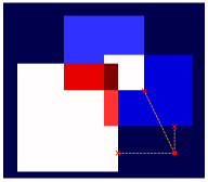
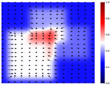
Figure 2: An example of how the FT baseline method (explained in Section 5.1) and our method handle an adaptive boosting ensemble with three trees. Left: decision boundary of the ensemble. Middle: three positive leaves that form the decision boundary, an example instance and the perturbed examples suggested by FT. Right: approximated loss $\widetilde{\mathcal{L}}_{pred}$ and its gradient w.r.t. $\bar{x}$. The FT perturbed examples do not change the prediction of the forest, whereas the gradient of the differentiable approximation leads toward the true decision boundary.

4.3 Approximations of Tree-based Models

If $f$ is not differentiable, we are unable to calculate its gradient with respect to the input $x$. However, the non-differentiable operations in our formulation are (i) the indicator function, and (ii) a maximum operation, both of which can be approximated by differentiable functions. First, we introduce the $\widetilde{t}_{j}(x)$ function that approximates the activation of node $j$: $\widetilde{t}_{j}(x)\approx t_{j}(x)$, using a sigmoid function with parameter $\sigma\in\mathbb{R}_{>0}$: $\textit{sig}(z)=(1+\exp(\sigma\cdot z))^{-1}$ and

$$\widetilde{t}_{j}(x) {}=\begin{cases}1,&\text{if $j$ is the root},\\ \widetilde{t}_{p_{j}}(x)\cdot\textit{sig}(\theta_{j}{-}x_{f_{j}}),&\text{if $j$ is left child},\\ \widetilde{t}_{p_{j}}(x)\cdot\textit{sig}(x_{f_{j}}{-}\theta_{j}),&\text{if $j$ is right child}.\end{cases}$$ (16)

As $\sigma$ increases, $\widetilde{t}_{j}$ approximates $t_{j}$ more closely. Next, we introduce a tree approximation:

$$\widetilde{\mathcal{T}}(y\mid x)=\sum_{j\in\mathcal{T}_{\mathit{leaf}}}\widetilde{t}_{j}(x)\cdot\mathcal{T}(y\mid j).$$ (17)

The approximation $\widetilde{\mathcal{T}}$ uses the same tree structure and thresholds as $\mathcal{T}$. However, its activations are no longer deterministic but instead are dependent on the distance between the feature values $x_{f_{j}}$ and the thresholds $\theta_{j}$. Lastly, we replace the maximum operation of $f$ by a softmax with temperature $\tau\in\mathbb{R}_{>0}$, resulting in:

$$\tilde{f}(y\mid x)=\frac{\exp\left(\tau\cdot\sum_{m=1}^{M}\omega_{m}\cdot\widetilde{\mathcal{T}}_{m}(y\mid x)\right)}{\sum_{y^{\prime}}\exp\left(\tau\cdot\sum_{m=1}^{M}\omega_{m}\cdot\widetilde{\mathcal{T}}_{m}(y^{\prime}\mid x)\right)}.$$ (18)

The approximation $\tilde{f}$ is based on the original model $f$ and the parameters $\sigma$ and $\tau$. This approximation is applicable to any tree-based model, and how well $\tilde{f}$ approximates $f$ depends on the choice of $\sigma$ and $\tau$. The approximation is potentially perfect since

$$\lim_{\sigma,\tau\rightarrow\infty}\tilde{f}(y\mid x)=f(y\mid x).$$ (19)

4.4 Our Method: FOCUS

We call our method FOCUS: Flexible Optimizable CounterfactUal Explanations for Tree EnsembleS. It takes as input an instance $x$, a tree-based classifier $f$, and two hyperparameters: $\sigma$ and $\tau$ which we use to create the approximation $\tilde{f}$. Following Equation 11, FOCUS outputs the optimal counterfactual example $\bar{x}^{*}$, from which we derive the optimal counterfactual explanation $\Delta^{*}_{x}=\bar{x}^{*}-x$.

4.5 Effects of Hyperparameters

Increasing $\sigma$ in $\tilde{f}$ eventually leads to exact approximations of the indicator functions, while increasing $\tau$ in $\tilde{f}$ leads to a completely unimodal softmax distribution. It should be noted that our approximation $\tilde{f}$ is not intended to replace the original model $f$ but rather to create a differentiable version of $f$ from which we can generate counterfactual examples through optimization. In practice, the original model $f$ would still be used to make predictions and the approximation would solely be used to generate counterfactual examples.

5 Experimental Setup

We consider 42 experimental settings to find the best counterfactual explanations using FOCUS. We jointly tune the hyperparameters of FOCUS ($\sigma,\tau,\beta,\alpha$) using Adam (Kingma and Ba 2015) for 1,000 iterations. We choose the hyperparameters that produce (i) a valid counterfactual example for every instance in the dataset, and (ii) the smallest mean distance between corresponding pairs ($x$, $\bar{x}$).

We evaluate FOCUS on four binary classification datasets: Wine Quality (UCI 2009), HELOC (FICO 2017a), COMPAS (Ofer 2017), and Shopping (UCI 2019). For each dataset, we train three types of tree-based models: Decision Trees (DT), Random Forests (RF), and Adaptive Boosting Trees (AB) with DTs as the base learners. We compare against two baselines that generate counterfactual examples for tree ensembles based on the inner workings of the model: Feature Tweaking (FT) by Tolomei et al. (2017) and Distribution-Aware Counterfactual Explanations (DACE) by Kanamori et al. (2020).

5.1 Baseline: Feature Tweaking

Feature Tweaking identifies the leaf nodes where the prediction of the leaf nodes do not match the original prediction $y_{x}$: it recognizes the set of leaves that if activated, $t_{j}(\bar{x})=1$, would change the prediction of a tree $\mathcal{T}$:

$$\mathcal{T}_{\textit{change}}=\left\{j\mid j\in\mathcal{T}_{\textit{leaf}}\land y_{x}\not=\arg\max_{y}T(y\mid j)\right\}.$$ (20)

For every $\mathcal{T}$ in $f$, FT generates a perturbed example per node in $\mathcal{T}_{\textit{change}}$ so that it is activated with at least an $\epsilon$ difference per threshold, and then selects the most optimal example (i.e., the one closest to the original instance). For every feature threshold $\theta_{j}$ involved, the corresponding feature is perturbed accordingly: $\bar{x}_{f_{j}}=\theta_{j}\pm\epsilon$. The result is a perturbed example that was changed minimally to activate a leaf node in $\mathcal{T}_{\textit{change}}$. In our experiments, we test $\epsilon\in\{0.001,0.005,0.01,0.1\}$, and choose the $\epsilon$ that minimizes the mean distance to the original input, while maximizing the number of counterfactual examples generated.

The main problem with FT is that the perturbed examples are not necessarily counterfactual examples, since changing the prediction of a single tree $\mathcal{T}$ does not guarantee a change in the prediction of the full ensemble $f$. Figure 2 shows all three perturbed examples generated by FT for a single instance. In this case, none of the generated examples change the model prediction and therefore none are valid counterfactual examples.

Figure 2 shows how FOCUS and FT handle an adaptive boosting ensemble using a two-feature ensemble with three trees. On the left is the decision boundary for a standard tree ensemble; the middle visualizes the positive leaf nodes that form the decision boundary; on the right is the approximated loss $\widetilde{\mathcal{L}}_{pred}$ and its gradient w.r.t. $\bar{x}$. The gradients push features close to thresholds harder and in the direction of the decision boundary if $\widetilde{\mathcal{L}}$ is convex.

5.2 Baseline: DACE

DACE generates counterfactual examples that account for the underlying data distribution through a novel cost function using Mahalanobis distance and a local outlier factor (LOF):

$$\begin{split}&d_{\mathit{DACE}}(x,\bar{x}|X,C)=\\ &{d_{\mathit{Mahalanobis}}}^{2}(x,\bar{x}|C)+\lambda q_{k}(x,\bar{x}|X),\end{split}$$ (21)

where $C$ is the covariance matrix, $q_{k}$ is the $k$-LOF (Breunig et al. 2000), $X$ is the training set, and $\lambda$ is the trade-off parameter. The $k$-LOF measures the degree to which an instance is an outlier in the context of its $k$-nearest neighbors. To generate counterfactual examples, DACE formulates the task as a mixed-integer linear optimization problem and uses the CPLEX Optimizer to solve it. We refer the reader to the original paper for a more detailed overview of this cost function. The $q_{k}$ term in the loss function penalizes counterfactual examples that are outliers, and therefore decreasing $\lambda$ results in a greater number of counterfactual examples. In our experiments, we test $\lambda\in\{0.001,0.01,0.1,0.5,1.0\}$, and choose the $\lambda$ that minimizes the mean distance to the original input, while maximizing the number of counterfactual examples generated. The main issue with DACE is that even for very small values of $\alpha$, it is unable to generate counterfactual examples for the majority of instances in the test sets (see Table 2). The other issue is that it is unable to run on some of our models because the problem size is too large when using the free Python API of CPLEX.

5.3 Datasets

We evaluate FOCUS on four binary classification tasks using the following datasets: Wine Quality (UCI 2009), HELOC (FICO 2017a), COMPAS (Ofer 2017), and Shopping (UCI 2019). The Wine Quality dataset (4,898 instances, 11 features) is about predicting the quality of white wine on a 0–10 scale. We adapt this to a binary classification setting by labelling the wine as “high quality” if the quality is $\geq$ 7. The HELOC set (10,459 instances, 23 features) is from the Explainable Machine Learning Challenge at NeurIPS 2017, where the task is to predict whether or not a customer will default on their loan. The COMPAS dataset (6,172 instances, 6 features) is used for detecting bias in ML systems, where the task is predicting whether or not a criminal defendant will reoffend upon release. The Shopping dataset (12,330 instances, 9 features) entails predicting whether or not an online website visit results in a purchase. We scale all features such that their values are in the range $\left[0,1\right]$ and remove categorical features.

5.4 Models

We train three types of tree-based models on 70% of each dataset: Decision Trees (DTs), Random Forests (RFs), and Adaptive Boosting (AB) with DTs as the base learners. We use the remaining 30% to find counterfactual examples for this test set. In total we have 12 models (4 datasets $\times$ 3 tree-based models). See Appendix A for more details.

5.5 Evaluation Metrics

We evaluate the counterfactual examples produced by FOCUS based on how close they are to the original input using three metrics. Mean distance, $d_{\mathit{mean}}$, measures the distance from the original input, averaged over all examples. Mean relative distance, $d_{\mathit{Rmean}}$, measures pointwise ratios of distance to the original input. This helps us interpret individual improvements over the baselines; if $d_{\mathit{Rmean}}<1$, FOCUS’s counterfactual examples are on average closer to the original input compared to the baseline. We also evaluate the proportion of FOCUS’s counterfactual examples that are closer to the original input compared to the baselines ($\mathit{\%_{closer}}$). We test the metrics in terms of four distance functions: Euclidean, Cosine, Manhattan and Mahalanobis.

			Euclidean			Cosine			Manhattan
Dataset	Metric	Method	DT	RF	AB	DT	RF	AB	DT	RF	AB
	$d_{mean}$	FT	0.269	0.174	0.267⊗	0.030	0.017	0.034⊗	0.269	0.223	0.382⊗
Wine		FOCUS	0.268∘	0.188▲	0.188▼	0.003▼	0.008▼	0.014▼	0.268∘	0.312▲	0.360▼
Quality	$d_{Rmean}$	FOCUS/FT	0.990	1.256	0.649	0.066	0.821	0.312	0.990	1.977	0.924
	$\mathit{\%_{closer}}$	FOCUS <FT	100%	21.0%	87.5%	100%	80.8%	95.1%	100%	5.4%	58.6%
	$d_{mean}$	FT	0.120	0.210	0.185	0.003	0.008	0.007	0.135	0.278	0.198
HELOC		FOCUS	0.133▲	0.186▼	0.136▼	0.001▼	0.002▼	0.001▼	0.152▲	0.284∘	0.203∘
	$d_{Rmean}$	FOCUS/FT	1.169	0.942	0.907	0.303	0.285	0.421	1.252	1.144	1.364
	$\mathit{\%_{closer}}$	FOCUS <FT	16.6%	57.9%	71.9%	91.6%	91.5%	92.9%	51.3%	43.6%	24.2%
	$d_{mean}$	FT	0.082	0.075	0.081	0.013	0.014	0.015	0.086	0.078	0.085
COMPAS		FOCUS	0.092▲	0.079∘	0.076▼	0.008▼	0.011▼	0.007▼	0.093▲	0.085∘	0.090∘
	$d_{Rmean}$	FOCUS/FT	1.162	1.150	1.062	0.473	0.965	0.539	1.182	1.236	1.155
	$\mathit{\%_{closer}}$	FOCUS <FT	29.4%	22.6%	44.8%	82.7%	68.0%	84.8%	65.8%	36.2%	66.9%
	$d_{mean}$	FT	0.119	0.028	0.126⊗	0.050	0.027	0.131⊗	0.121	0.030	0.142⊗
Shopping		FOCUS	0.142▲	0.025▼	0.028▼	0.055▲	0.013▼	0.006▼	0.128∘	0.026▼	0.046▼
	$d_{Rmean}$	FOCUS/FT	1.051	1.053	0.218	0.795	0.482	0.074	0.944	0.796	0.312
	$\mathit{\%_{closer}}$	FOCUS <FT	40.2%	36.1%	99.6%	44.4%	86.1%	99.5%	55.8%	81.9%	97.1%

Table 1: Evaluation results for Experiment 1 comparing FOCUS and FT counterfactual examples. Significant improvements and losses over the baseline (FT) are denoted by ^▼ and ^▲, respectively ($p<0.05$, two-tailed t-test,); ^∘ denotes no significant difference; ^⊗ denotes settings where the baseline cannot find a counterfactual example for every instance.

		Wine	HELOC	COMPAS		Shopping
Metric	Method	DT	DT	DT	AB	DT	AB
$d_{mean}$	DACE	1.325	1.427	0.814	1.570	0.050	3.230
	FOCUS	0.542▼	0.810▼	0.776∘	0.636▼	0.023▼	0.303▼
$d_{Rmean}$	FOCUS /	0.420	0.622	1.18	0.372	0.449	0.380
	DACE
$\mathit{\%_{closer}}$	FOCUS <	100%	94.5%	29.9%	96.1%	99.4%	90.8%
	DACE
# CFs	DACE	241	1,342	842	700	362	448
found	FOCUS	1,470	3,138	1,852	1,852	3,699	3,699
# obs in	dataset	1,470	3,138	1,852	1,852	3,699	3,699

Table 2: Evaluation results for Experiment 2 comparing FOCUS and DACE counterfactual examples in terms of Mahalanobis distance. Significant improvements over the baseline are denoted by ^▼ ($p<0.05$, two-tailed t-test,). ^∘ denotes no significant difference.

6 Experiment 1: FOCUS vs. FT

We compare FOCUS to the Feature Tweaking (FT) method by Tolomei et al. (2017) in terms of the evaluation metrics in Section 5.5. We consider 36 experimental settings (4 datasets $\times$ 3 tree-based models $\times$ 3 distance functions) when comparing FOCUS to FT. The results are listed in Table 1.

In terms of $d_{\mathit{mean}}$, FOCUS outperforms FT in 20 settings while FT outperforms FOCUS in 8 settings. The difference in $d_{\mathit{mean}}$ is not significant in the remaining 8 settings. In general, FOCUS outperforms FT in settings using Euclidean and Cosine distance because in each iteration, FOCUS perturbs many of the features by a small amount. Since FT perturbs only the features associated with an individual leaf, we expected that it would perform better for Manhattan distance but our results show that this is not the case – there is no clear winner between FT and FOCUS for Manhattan distance. We also see that FOCUS usually outperforms FT in settings using Random Forests (RF) and Adaptive Boosting (AB), while the opposite is true for Decision Trees (DT).

Overall, we find that FOCUS is effective and efficient for finding counterfactual explanations for tree-based models. Unlike the FT baseline, FOCUS finds valid counterfactual explanations for every instance across all settings. In the majority of tested settings, FOCUS’s explanations are substantial improvements in terms of distance to the original inputs, across all three metrics.

7 Experiment 2: FOCUS vs. DACE

The flexibility of FOCUS allows us to plug in our choice of differentiable distance function. To compare against DACE (Kanamori et al. 2020), we use the Mahalanobis distance for both (i) generation of FOCUS explanations, and (ii) evaluation in comparison to DACE, since this is the distance function used in the DACE loss function (see Equation 21 in Section 5.2).

Table 2 shows the results for the 6 settings we could run DACE on. We were only able to run DACE on 6 out of our 12 models because the problem size is too large (i.e., DACE has too many model parameters) for the remaining 6 models when using the free Python API of CPLEX (the optimizer used in DACE). Therefore, when comparing against DACE, we have 6 experimental settings (6 models $\times$ 1 distance function).

We found that DACE can only generate counterfactual examples for a small subset of the test set, regardless of the $\lambda$-value, as opposed to FOCUS, which can generate counterfactual examples for the entire test set in all cases. To compute $d_{mean}$, $d_{Rmean}$, and $\mathit{\%_{closer}}$, we compare FOCUS and DACE only on the instances for which DACE was able to generate a counterfactual example. We find that FOCUS significantly outperforms DACE in 5 out of 6 settings in terms of all three evaluation metrics, indicating that FOCUS explanations are indeed more minimal than those produced by DACE. FOCUS is also more reliable since (i) it is not restricted by model size, and (ii) it can generate counterfactual examples for all instances in the test set.

8 Discussion and Analysis

Figure 3 shows the mean Manhattan distance of the perturbed examples in each iteration of FOCUS, along with the proportion of perturbations resulting in valid counterfactual examples found for two datasets (we omit the others due to space considerations). These trends are indicative of all settings: the mean distance increases until a counterfactual example has been found for every $x$, after which the mean distance starts to decrease. This seems to be a result of the hinge-loss in FOCUS, which first prioritizes finding a valid counterfactual example (see Equation 1), then decreasing the distance between $x$ and $\bar{x}$.

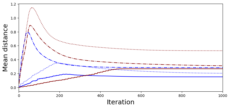
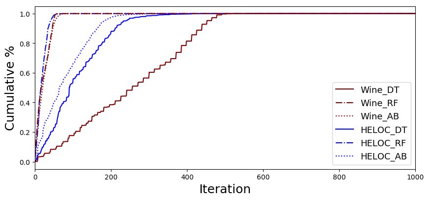
Figure 3: Mean distance (top) and cumulative % (bottom) of counterfactual examples in each iteration of FOCUS for Manhattan explanations.

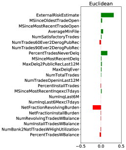
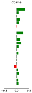
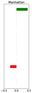
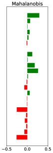
Figure 4: FOCUS explanations for the same model and same $x$ based on different distance functions. Green and red indicate increases and decreases in feature values, respectively. Perturbation values are based on normalized feature values. Left: Euclidean explanation perturbs several features, but only slightly. Middle Left: Cosine explanation perturbs almost all of the features. Middle Right: Manhattan explanation perturbs two features substantially. Right: Mahalanobis explanation perturbs almost all of the features.

8.1 Case Study: Credit Risk

As a practical example, we investigate what FOCUS explanations look like for individuals in the HELOC dataset. Here, the task is to predict whether or not an individual will default on their loan. This has consequences for loan approval: individuals who are predicted as defaulting will be denied a loan. For these individuals, we want to understand how they can change their profile such that they are approved. Given an individual who has been denied a loan from a bank, a counterfactual explanation could be:

Your loan application has been denied. In order to have your loan application approved, you need to (i) increase your ExternalRiskEstimate score by 62, and (ii) decrease your NetFractionRevolvingBurden by 58.

Figure 4 shows four counterfactual explanations generated using different distance functions for the same individual and same model. We see that the Manhattan explanation only requires a few changes to the individual’s profile, but the changes are large. In contrast, the individual changes in the Euclidean explanation are smaller but there are more of them. In settings where there are significant dependencies between features, the Cosine explanations may be preferred since they are based on perturbations that try to preserve the relationship between features. For instance, in the Wine Quality dataset, it would be difficult to change the amount of citric acid without affecting the pH level. The Mahalanobis explanations would be useful when it is important to take into account not only correlations between features, but also the training data distribution. This flexibility allows users to choose what kind of explanation is best suited for their problem.

Different distance functions can result in different magnitudes of feature perturbations as well as different directions. For example, the Cosine explanation suggests increasing PercentTradesWBalance, while the Mahalanobis explanations suggests decreasing it. This is because the loss space of the underlying RF model is highly non-convex, and therefore there is more than one way to obtain an alternative prediction. When using complex models such as tree ensembles, there are no monotonicity guarantees. In this case, both options result in valid counterfactual examples.

We examine the Manhattan explanation in more detail. We see that FOCUS suggests two main changes: (i) increasing the ExternalRiskEstimate, and (ii) decreasing the NetFractionRevolvingBurden. We obtain the definitions and expected trends from the data dictionary (FICO 2017b) created by the authors of the dataset. The ExternalRiskEstimate is a “consolidated version of risk markers” (i.e., a credit score). A higher score is better: as one’s ExternalRiskEstimate increases, the probability of default decreases. The NetFractionRevolvingBurden is the “revolving balance divided by the credit limit” (i.e., utilization). A lower value is better: as one’s NetFractionRevolvingBurden increases, the probability of default increases. We find that the changes suggested by FOCUS are fairly consistent with the expected trends in the data dictionary (FICO 2017b), as opposed to suggesting nonsensical changes such as increasing one’s utilization to decrease the probability of default.

Decreasing one’s utilization is heavily dependent on the specific situation: an individual who only supports themselves might have more control over their spending in comparison to someone who has multiple dependents. An individual can decrease their utilization in two ways: (i) decreasing their spending, or (ii) increasing their credit limit (or a combination of the two). We can postulate that (i) is more “actionable” than (ii), since (ii) is usually a decision made by a financial institution. However, the degree to which an individual can actually change their spending habits is completely dependent on their specific situation: an individual who only supports themselves might have more control over their spending than someone who has multiple dependents. In either case, we argue that deciding what is (not) actionable is not a decision for the developer to make, but for the individual who is affected by the decision. Counterfactual examples should be used as part of a human-in-the-loop system and not as a final solution. The individual should know that utilization is an important component of the model, even if it is not necessarily “actionable” for them. We also note that it is unclear how exactly an individual would change their credit score without further insight into how the score was calculated (i.e., how the risk markers were consolidated). It should be noted that this is not a shortcoming of FOCUS, but rather of using features that are uninterpretable on their own, such as credit scores. Although FOCUS explanations cannot tell a user precisely how to increase their credit score, it is still important for the individual to know that their credit score is an important factor in determining their probability of getting a loan, as this empowers them to ask questions about how the score was calculated (i.e., how the risk markers were consolidated).

9 Conclusion

We propose an explanation method for tree-based classifiers, FOCUS, which casts the problem of finding counterfactual examples as a gradient-based optimization task and provides a differentiable approximation of tree-based models to be used in the optimization framework. Given an input instance $x$, FOCUS generates an optimal counterfactual example based on the minimal perturbation to the input instance $x$ which results in an alternative prediction from a model $f$. Unlike previous methods that assume the underlying classification model is differentiable, we propose a solution for when $f$ is a non-differentiable, tree-based model that provides a differentiable approximation of $f$ that can be used to find counterfactual examples using gradient-based optimization techniques. In the majority of experiments, examples generated by FOCUS are significantly closer to the original instances in terms of three different evaluation metrics compared to those generated by the baselines. FOCUS is able to generate valid counterfactual examples for all instances across all datasets, and the resulting explanations are flexible depending on the distance function. We plan to conduct a user study to test how varying the distance functions impacts user preferences for explanations.

Reproducibility

To facilitate the reproducibility of this work, our code is available at https://github.com/a-lucic/focus.

References

- Alaa, Weisz, and van der Schaar (2017) Alaa, A. M.; Weisz, M.; and van der Schaar, M. 2017. Deep Counterfactual Networks with Propensity-Dropout. In ICML Workshop on Principled Approaches to Deep Learning.
- Balestriero (2017) Balestriero, R. 2017. Neural Decision Trees. arXiv preprint arXiv:1702.07360.
- Biggio and Roli (2018) Biggio, B.; and Roli, F. 2018. Wild Patterns: Ten Years After the Rise of Adversarial Machine Learning. Pattern Recognition, 84: 317–331.
- Breunig et al. (2000) Breunig, M. M.; Kriegel, H.-P.; Ng, R. T.; and Sander, J. 2000. LOF: Identifying Density-Based Local Outliers. SIGMOD Rec., 29(2): 93–104.
- Brown et al. (2018) Brown, T. B.; Mané, D.; Roy, A.; Abadi, M.; and Gilmer, J. 2018. Adversarial Patch. In Advances in Neural Information Processing Systems 31.
- Dhurandhar et al. (2018) Dhurandhar, A.; Chen, P.-Y.; Luss, R.; Tu, C.-C.; Ting, P.; Shanmugam, K.; and Das, P. 2018. Explanations based on the Missing: Towards Contrastive Explanations with Pertinent Negatives. In Advances in Neural Information Processing Systems 31, 592–603. Curran Associates, Inc.
- Doshi-Velez and Kim (2018) Doshi-Velez, F.; and Kim, B. 2018. Considerations for Evaluation and Generalization in Interpretable Machine Learning, 3–17. Cham: Springer International Publishing. ISBN 978-3-319-98131-4.
- EU (2016) EU. 2016. Regulation (EU) 2016/679 of the European Parliament and of the Council of 27 April 2016 on the protection of natural persons with regard to the processing of personal data and on the free movement of such data, and repealing Directive 95/46/EC (General Data Protection Regulation). Official Journal of the European Union, L119: 1–88.
- FICO (2017a) FICO. 2017a. Explainable Machine Learning Challenge.
- FICO (2017b) FICO. 2017b. FICO xML Challenge.
- Goodfellow, Shlens, and Szegedy (2015) Goodfellow, I. J.; Shlens, J.; and Szegedy, C. 2015. Explaining and Harnessing Adversarial Examples. In 3rd International Conference on Learning Representations.
- Grath et al. (2018) Grath, R. M.; Costabello, L.; Van, C. L.; Sweeney, P.; Kamiab, F.; Shen, Z.; and Lecue, F. 2018. Interpretable Credit Application Predictions With Counterfactual Explanations. In NeurIPS Workshop on Challenges and Opportunities for AI in Financial Services.
- Hinton, Vinyals, and Dean (2014) Hinton, G.; Vinyals, O.; and Dean, J. 2014. Distilling the Knowledge in a Neural Network. In NeurIPS Workshop on Deep Learning.
- Joshi et al. (2020) Joshi, S.; Koyejo, O.; Vijitbenjaronk, W.; Kim, B.; and Ghosh, J. 2020. Towards Realistic Individual Recourse and Actionable Explanations in Black-Box Decision Making Systems. In Proceedings of the 23rd International Conference on Artificial Intelligence and Statistics.
- Kanamori et al. (2020) Kanamori, K.; Takagi, T.; Kobayashi, K.; and Arimura, H. 2020. DACE: Distribution-Aware Counterfactual Explanation by Mixed-Integer Linear Optimization. In Proceedings of the Twenty-Ninth International Joint Conference on Artificial Intelligence, 2855–2862. International Joint Conferences on Artificial Intelligence Organization. ISBN 978-0-9992411-6-5.
- Karimi et al. (2020a) Karimi, A.-H.; Barthe, G.; Balle, B.; and Valera, I. 2020a. Model-Agnostic Counterfactual Explanations for Consequential Decisions. In Proceedings of the 23rd International Conference on Artificial Intelligence and Statistics.
- Karimi, Schölkopf, and Valera (2021) Karimi, A.-H.; Schölkopf, B.; and Valera, I. 2021. Algorithmic Recourse: From Counterfactual Explanations to Interventions. In Proceedings of the 2021 ACM Conference on Fairness, Accountability, and Transparency, FAccT ’21, 353–362. New York, NY, USA: Association for Computing Machinery. ISBN 9781450383097.
- Karimi et al. (2020b) Karimi, A.-H.; von Kügelgen, J.; Schölkopf, B.; and Valera, I. 2020b. Algorithmic recourse under imperfect causal knowledge: a probabilistic approach. In Advances in Neural Information Processing Systems 33. Curran Associates, Inc.
- Kingma and Ba (2015) Kingma, D. P.; and Ba, J. 2015. Adam: A Method for Stochastic Optimization. In Bengio, Y.; and LeCun, Y., eds., 3rd International Conference on Learning Representations.
- Laugel et al. (2018) Laugel, T.; Lesot, M.-J.; Marsala, C.; Renard, X.; and Detyniecki, M. 2018. Inverse Classification for Comparison-based Interpretability in Machine Learning. In 17th International Conference on Information Processing and Management of Uncertainty in Knowledge-Based Systems (IPMU 2018).
- Madumal et al. (2019) Madumal, P.; Miller, T.; Sonenberg, L.; and Vetere, F. 2019. Explainable Reinforcement Learning Through a Causal Lens. In AAAI Conference on Artificial Intelligence.
- Mothilal, Sharma, and Tan (2020) Mothilal, R. K.; Sharma, A.; and Tan, C. 2020. Explaining Machine Learning Classifiers through Diverse Counterfactual Explanations. In Proceedings of the 2020 Conference on Fairness, Accountability, and Transparency, FAT* ’20, 607–617. New York, NY, USA: Association for Computing Machinery. ISBN 9781450369367.
- Ofer (2017) Ofer, D. 2017. COMPAS Dataset. https://www.kaggle.com/danofer/compass.
- Poyiadzi et al. (2020) Poyiadzi, R.; Sokol, K.; Santos-Rodriguez, R.; De Bie, T.; and Flach, P. 2020. FACE: Feasible and Actionable Counterfactual Explanations. In Proceedings of the AAAI/ACM Conference on AI, Ethics, and Society.
- Russell (2019) Russell, C. 2019. Efficient Search for Diverse Coherent Explanations. In Proceedings of the Conference on Fairness, Accountability, and Transparency, FAT* ’19, 20–28. New York, NY, USA: Association for Computing Machinery. ISBN 9781450361255.
- Su, Vargas, and Kouichi (2019) Su, J.; Vargas, D. V.; and Kouichi, S. 2019. One Pixel Attack for Fooling Deep Neural Networks. IEEE Transactions on Evolutionary Computation, 23(5): 828–841.
- Szegedy et al. (2014) Szegedy, C.; Zaremba, W.; Sutskever, I.; Bruna, J.; Erhan, D.; Goodfellow, I.; and Fergus, R. 2014. Intriguing Properties of Neural Networks. In 2nd International Conference on Learning Representations.
- Tolomei et al. (2017) Tolomei, G.; Silvestri, F.; Haines, A.; and Lalmas, M. 2017. Interpretable Predictions of Tree-based Ensembles via Actionable Feature Tweaking. In Proceedings of the 23rd ACM SIGKDD International Conference on Knowledge Discovery and Data Mining - KDD ’17, 465–474. ACM.
- UCI (2009) UCI. 2009. Wine Quality Data Set. https://archive.ics.uci.edu/ml/datasets/Wine+Quality.
- UCI (2019) UCI. 2019. Online Shoppers Intention Dataset. https://archive.ics.uci.edu/ml/datasets/Online+Shoppers+Purchasing+Intention+Dataset.
- Ustun, Spangher, and Liu (2019) Ustun, B.; Spangher, A.; and Liu, Y. 2019. Actionable Recourse in Linear Classification. In Proceedings of the Conference on Fairness, Accountability, and Transparency, FAT* ’19, 10–19. New York, NY, USA: Association for Computing Machinery. ISBN 9781450361255.
- Van Looveren and Klaise (2021) Van Looveren, A.; and Klaise, J. 2021. Interpretable Counterfactual Explanations Guided by Prototypes. In Oliver, N.; Pérez-Cruz, F.; Kramer, S.; Read, J.; and Lozano, J. A., eds., Machine Learning and Knowledge Discovery in Databases. Research Track, 650–665. Cham: Springer International Publishing. ISBN 978-3-030-86520-7.